A mixed non-homogeneous Poisson process to model the quality of maintenance

Abstract

We present a model for the corrective and preventive maintenance of a system. The latter is based on a bivariate policy that replaces the system either at age $T$ or after the $M$ failure, whichever comes first. A repair follows each of the $M - 1$ first failures, restoring the system operational state, but with a lower reliability than before failing. We present two scenarios with constant and time-dependent repair costs. The results reveal that systems with low initial reliability can greatly benefit from the bivariate policy. The advantage decreases for poor quality repairs. We also obtain conditions to obtain the optimum number $M$ when $T$ is given. This result is helpful to assess whether a system should be replaced sooner than originally planned.

Keywords

age replacement mixture non-homogeneous Poisson process generalized Pólya process (GPP)optimum policy

Introduction

Systems are usually repaired several times before being replaced. The extended time of use thus obtained must be weighed against the costs derived from failures and repairs to determine the optimum time for system renewal. Both, preventive and corrective maintenance are becoming increasingly important in the current world, where sustainability is driving the need to extend the life of all types of equipment.

The positive effect of maintenance on reliability is a general assumption in most models. It ranges from the minimal repair, that restores exactly the same reliability previous to failure, to system renewal and any other reliability level in between. However, the possibility of maintenance that leaves the system in a worse condition than before failing has received little attention in the literature. Cha et al.¹ justify this assumption by the negative effects of previous repairs, environmental and internal shocks, etc. Badía et al.² mention the lack of either adequate resources or properly trained maintainers as a reason for this poor maintenance.

The maintenance of roads and pipes shows this adverse effect. Potholes on highways are a serious safety risk to drivers, and they are constantly patched. It is also common to see the same point of the road being repaired repeatedly. This occurs because the patch is less reliable than the original pavement³ or because the asphalt layer thickness is not optimal.⁴ Khahro⁵ highlights the impact of a low-cost pavement management. The increasing use of recycled materials in pavements⁶ also leads to the assumption that these materials are less reliable when they are used in patches. Maintenance models have to assume the possibility that high-quality maintenance may not be carried out due to either limited budgets or studies that fail to detect the actual road deterioration.

Age replacement is a basic strategy for avoiding failures. Thus, the system is replaced when it fails or when it reaches a specified age, $T$ , whichever comes first. However, some systems cannot be maintained periodically, but are better maintained at a random time, for example when a working cycle is completed,⁷ when a software update is available⁸ or after $N$ failures.⁹ The works of Mituzani et al.,⁸ Zhao and Nakagawa,¹⁰ and Badía et al.² consider the combination of random and periodic or age-based replacement.

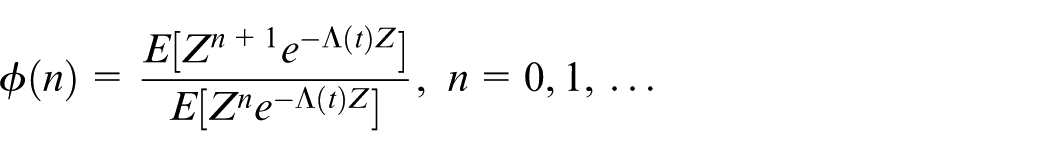
The minimal repair assumption implies that the system recovers its functional state, but the failure rate remains undisturbed, equal to that of a system of the same age (as-bad-as-old). Potential industrial applications are found in systems consisting of a large number of components and a failed system is restored to the operating condition by replacing only the failed component. The non-homogeneous Poisson process (NHPP) models failures in systems undergoing minimal repairs.¹¹ It is useful to overcome the memoryless assumption when the deterioration process is not Markovian.¹² Overlooking heterogeneity between systems when analyzing failure data can lead to inaccurate estimations.¹³ The generalized Pólya process (GPP) extends the NHPP by assuming that time varying environments affect the reliability of systems.^2,14 System functionality can be restored in different ways. For example, the component that replaced the failed one can be new or refurbished, or the maintenance team can have different levels of expertise. This variability in the quality of the repair is responsible for a heterogeneous population of systems and it must also be taken into account when designing maintenance policies; otherwise, they will not achieve the desired result. In particular, assuming that a minimal repair applies and, thus, a failure process following a NHPP, can overestimate the reliability of a system that is actually in a worse-than-old condition rather than as-bad-as-old. Unobserved heterogeneity between systems cannot be controlled and it is modeled by a frailty, $Z$ . $Z$ is a random variable which takes a particular value $z$ for each system over its entire life, but changes between systems, explaining their differences. Therefore, assuming a mixture of non-homogeneous Poison processes (MNHPP) can be more realistic than using a single NHPP. In terms of managerial implications, a MNHPP can account for deficient maintenance and provide a dramatically different timescale for replacing a system. The relevance of considering heterogeneous populations in maintenance has recently been highlighted in Lee et al.¹⁵ and Santos and Cavalcante.¹⁶

This paper presents two models that combine random and non-random maintenance of a system that undergoes minimal repairs after each of the first $M - 1$ failures. The system is replaced after the first of the following two events occurs: the $M$ failure or reaching age $T$ . Thus, the system is no longer used when either its age or failure history induces high maintenance costs. This policy emulates the usual procedure of maintainers. Random replacement after $M$ failures protects against frequent failures. This is particularly useful when failures happen in the early stages due to hidden defects that occur during the design stage or the manufacturing process or due to refurbished components.¹⁷ Regarding road maintenance, it eliminates the potholes that appear in new roads due to a defective pavement or insufficient asphalt layer thickness.

The models in this paper differ from those in previous references in the following major assumptions:

We assume a MNHPP for the time to the $M$ failure, which is an extension of the GPP repair process. The mixture is the result of differences in the quality of repairs. Thus, this new model accounts for random variability in repairing conditions, as well as time-varying reliability, which is more general than that in Badía et al.²

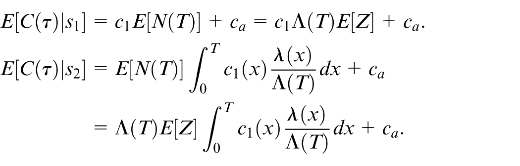
In model 2, we introduce time-dependent repair costs, $c_{1} (t)$ , in contrast to the constant value, $c_{1}$ , of model 1. This second assumption provides further insight into the comparison between deterministic and random preventive replacement.

From the point of view of real applications, we extend the idea of low quality maintenance in Santos and Cavalcante,¹⁶ by considering successive repairs that restore the operational state of a system but with lower reliability than before the failure occurred (worse-than-old).² The consequence is that the occurrence of failures increases after each repair. This effect leads to the resurfacing of long sections of roads, for example. In addition, the bivariate maintenance policy is a useful strategy to determine the maximum usage time of a component subject to low-quality maintenance. The maintainer can decide when no further repairs are cost-effective and replace the component with a new one.

This paper is organized as follows: Section 2 presents the key concepts of the MNHPP, which models the repairs in models 1 and 2. Section 3 contains the model building that leads to the cost function under the two scenarios, constant repair cost and time-dependent repair cost. It also presents the analysis of the conditions under which an optimum policy exists. The corresponding proofs as well as some basics on stochastic ordering, are in the Appendices A1, A2 and A3. The classical univariate policies, $(T^{★}, \infty)$ and $(\infty, M^{★})$ , are presented in Section 4. The sensitivity analysis in Section 5 analyzes the range of application of models 1 and 2 when comparing the optimum bivariate policy, $(T^{★}, M^{★})$ , with the corresponding classical univariate, $(T^{★}, \infty)$ and $(\infty, M^{★})$ . The conclusions are summarized in Section 6.

MNHPP repair model

First, we introduce the notation that will be used throughout this paper:

$N (t)$	number of failures in $[0, t]$
$λ (t)$	failure rate of the time to the first failure
$λ_{t}$	stochastic intensity
$Z$	unobservable covariates (frailty)
$λ (t, z)$	failure rate conditional to $Z = z$
$T_{n}$	time to the $n$ failure
$M$	maximum number of failures previous to replacement (decision variable)
$T$	time for preventive age replacement (decision variable)
$τ$	length of a renewal cycle
$c_{f}$	cost of renewal on the $M$ failure
$c_{a}$	cost of age replacement at $T$
$c_{1}$	constant cost of repair in scenario 1
$c_{1} (t)$	time dependent cost of repair in scenario 2
$C (τ)$	total cost of a cycle
$Q (T, M)$	cost rate (the long run expected cost per unit time)
DFR	decreasing failure rate
IFR	increasing failure rate

Let ${N (t) : t \geq 0}$ be a counting process with $N (t)$ the number of events in $[0, t]$ . In addition $H_{t}$ represents its filtration, that is, the history of the process given by $N (t)$ and $T_{1}, \dots T_{N (t^{-})}$ with $T_{i}$ the epoch time of the $i$ th event in the counting process.

The stochastic intensity, $λ_{t}$ , of a counting process ${N (t) : t \geq 0}$ , is defined as

λ_{t} = \lim_{h \to 0} \frac{P (N (t, t + h) = 1 | H_{t})}{h}

Observe that $h λ_{t}$ is the conditional probability of failure in an infinitesimal interval, $h$ , given the previous history of failures of the system. Hence, the intensity rate is similar to the failure rate concept although $λ_{t}$ accounts for the effect of the past failures in the current reliability of the system. In addition, assuming that repairing conditions cannot be perfectly controlled, but instead change randomly between systems, provides a more realistic model for failures, which are expected to occur more frequently in systems under low quality maintenance. The frailty, $Z$ , accounts for such heterogeneity in the counting process of the failures. $Z$ is assumed to be a non-negative random variable that leads to a mixture of counting processes. The work in Brown et al.¹³ is concerned with the choice of the frailty.

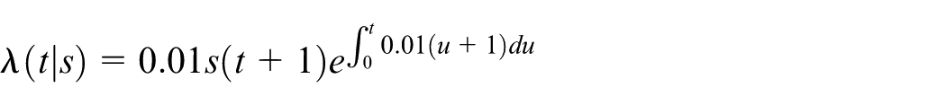
In what follows we assume that the frailty, $Z$ , has a multiplicative effect on the failure rate:

λ (t, z) = z λ (t)

$λ (t, z)$ is the failure rate when $Z = z$ , whereas the failure rate of the time until the first failure, $λ (t)$ , serves as baseline intensity. When $Z > 1$ , the failure rate is higher than the baseline. On the contrary, $Z < 1$ leads to a reduction in the failure rate.

We consider the particular case of a MNHPP as in Cha and Finkelstein.¹⁸ They provide an expression for the stochastic intensity (chapter 4, page 109) that, for the multiplicative model $λ (t, z) = z λ (t)$ , turns out to be

λ_{t} = λ (t) \frac{E [Z^{N (t) + 1} e^{- Λ (t) Z}]}{E [Z^{N (t)} e^{- Λ (t) Z}]}

(1)

with $Λ (t)$ being the cumulative baseline intensity:

Λ (t) = \int_{0}^{t} λ (x) dx

(2)

The stochastic intensity in equation (1) explains both the time aftermath, which is generally adverse for most systems, and random effects that can aggravate or alleviate the former. Note that for $Z = 1$ the expression in equation (1) corresponds to the intensity function of a non-homogeneous Poisson process which in turn describes the counting process of the failures for a system under minimal repair.

In what follows we will consider a system that is repaired after failing and keeps on working until the following failure. The mixed non-homogeneous repair process (MNHPP) is defined next.

Definition 1. The counting process ${N (t) : t \geq 0}$ with $N (t)$ being the number of failures in $[0, t]$ , is given by a MNHPP repair model with baseline intensity $λ (t)$ and frailty $Z$ , if $T_{n}$ ( $n = 1, \dots$ ) corresponds to the $n$ epoch time of the mixed non-homogeneous Poisson process with intensity $λ_{t}$ in (1).

The main property of the MNHPP repair process is given in the following proposition.

Proposition 1. Let ${N (t) : t \geq 0}$ be a MNHPP repair model. Then its stochastic intensity, $λ_{t}$ , increases with $N (t)$ .

The result holds since

ϕ (n) = \frac{E [Z^{n + 1} e^{- Λ (t) Z}]}{E [Z^{n} e^{- Λ (t) Z}]}, n = 0, 1, \dots

is increasing in $n$ .

Proof. Consider the ratio $\frac{ϕ (n + 1)}{ϕ (n)}$ for $n = 0, 1, \dots$ :

\frac{ϕ (n + 1)}{ϕ (n)} = \frac{E [Z^{n + 2} e^{- Λ (t) Z}]}{E [Z^{n + 1} e^{- Λ (t) Z}]} \frac{E [Z^{n} e^{- Λ (t) Z}]}{E [Z^{n + 1} e^{- Λ (t) Z}]}

The Cauchy-Schwartz inequality states:

E^{2} [Z^{n + 1} e^{- Λ (t) Z}] \leq E [Z^{n} e^{- Λ (t) Z}] E [Z^{n + 2} e^{- Λ (t) Z}] .

thus, $\frac{ϕ (n + 1)}{ϕ (n)} \geq 1$ , and the result follows.

Therefore, $λ_{t}$ is also increasing with $N (t)$ . The previous proposition implies that, although the system recovers its functionality after each repair, its condition is worse than before failing. Hence, the worse-than-old condition can be interpreted as the result of a mixture of minimal repairs in heterogeneous populations. This worse-than-old condition makes the difference between the MNHPP repair model and the minimal repair.

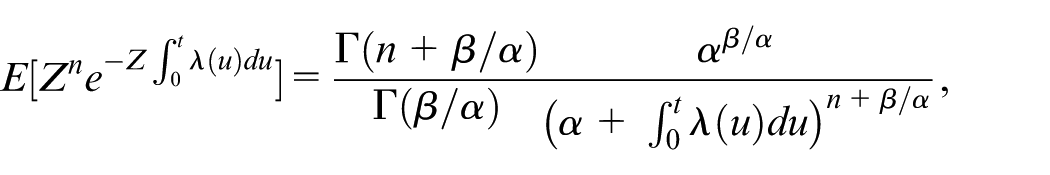
Furthermore, the MNHPP repair model is an extension of the GPP repair process considered in Lee and Cha.^19,20 In the particular case that the baseline failure rate in the NHPP be $λ (t) = α r (t) e^{\int_{0}^{t} r (u) du}$ and the frailty, $Z$ , a gamma random variable with scale parameter $α$ and shapeparameter $β / α$ , it follows that

E [Z^{n} e^{- Z \int_{0}^{t} λ (u) du}] = \frac{Γ (n + β / α)}{Γ (β / α)} \frac{α^{β / α}}{{(α + \int_{0}^{t} λ (u) du)}^{n + β / α}},

and then from equation (1) the stochastic intensity of the mixed NHPP process is

λ_{t} = (N (t) + \frac{β}{α}) r (t)

(3)

which is also the stochastic intensity of the generalized Pólya process (GPP) with parameters $(r (t)$ , 1, $\frac{β}{α})$ .

Model building

We consider a one component system undergoing a single type to failure that is minimally repaired after every failure with $λ (x)$ being the hazard rate of the time to the first failure. The higher $λ (x)$ , the greater the risk of failure.

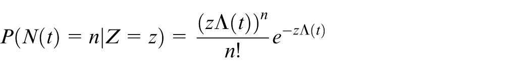
Definition 1 in Badía et al.,² states that the Generalized Pólya Process with parameters $(λ (t), α = 0, β = 1)$ is a non-homogeneous Poisson process with rate equal to $λ (t)$ . The corresponding probability of $n$ failures in $(0, t)$ is a Poisson distribution with mean $Λ (t) = \int_{0}^{t} λ (x) dx$ . The MNHPP in this paper and the corresponding repair process also extend the NHPP, which in turn emerges under the minimal repair. The probability of $N (t) = n$ failures $(n = 1, 2, \dots)$ when $Z = z$ is

P (N (t) = n | Z = z) = \frac{{(z Λ (t))}^{n}}{n!} e^{- z Λ (t)}

That is, the probability of $n$ failures in $(0, t)$ for a non-homogeneous Poisson process with rate equal to $z λ (t)$ .

Then, the unconditional probability of $N (t) = n$ failures is

P (N (t) = n) = \int_{0}^{\infty} \frac{{(z Λ (t))}^{n}}{n!} e^{- z Λ (t)} π (z) dz

with $π (z)$ the density function of $Z$ . Thus, the failure process, ${N (t) : t \geq 0}$ , is given by a mixture of non-homogeneous Poisson processes.

Each time the system fails, a minimal repair restores the system back to function. Proposition 1 states that the random effect of the repair given by $Z$ , leaves the system in a worse-than-old condition.

The following assumptions also apply to the maintenance procedure:

The system is replaced on the $M$ failure or at age $T$ whichever comes first.

Repair times are considered to be negligible.

The cost of preventive replacement on the $M$ failure and at age $T$ are, respectively, $c_{f}$ and $c_{a}$ .

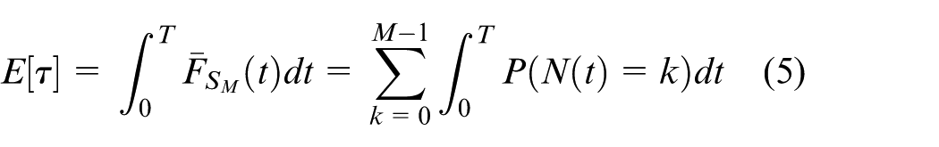
Although working times of most systems are finite, the study of optimum maintenance policies is simpler when an infinite time span is considered.²¹ Since we do not assume that the system must fulfill a specific task within a given period, the objective function to be analyzed is the incurred cost per unit of time in an infinite interval. The key theorem of the renewal reward processes²² guarantees that this function is equivalent to the next one:

Q (T, M) = \frac{E [C (τ)]}{E [τ]}

with $τ$ and $C (τ)$ being, respectively, the length and the cost of a renewal cycle. In addition $T$ and $M$ are decision variables. Therefore, given the costs of repair and replacement as well as the rest of parameters defining the failure process, the optimum values $T^{★}$ and $M^{★}$ minimizing $Q (T, M)$ have to be obtained.

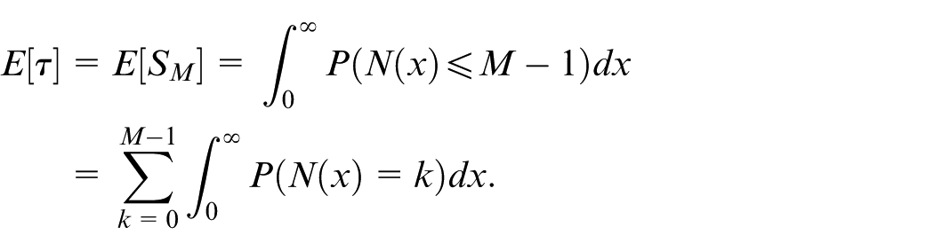
Let $S_{n}$ be the random time until the $n$ -th failure. Its density function is given by:

f_{S_{n}} (x) = \int_{0}^{\infty} \frac{z^{n} Λ {(x)}^{n - 1}}{(n - 1)!} λ (x) e^{- z Λ (x)} π (z) dz

(4)

$S_{n}$ and the process of failures, ${N (t) : t \geq 0}$ , verify

P (S_{M} \leq t) = P (N (t) \geq M)

Hence the probability that the $M$ failure occurs no later than $t$ is equivalent to the probability that $M$ failures occur at least before $t$ .

Then, the length of a renewal cycle

τ = \min (S_{M}, T)

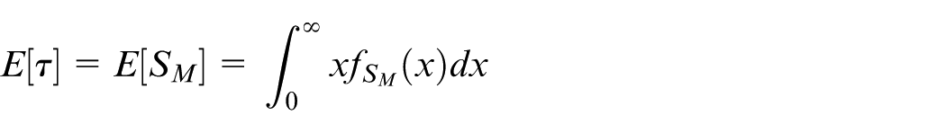
and its expected value

\begin{matrix} E [τ] = \int_{0}^{T} {\bar{F}}_{S_{M}} (t) dt = \sum_{k = 0}^{M - 1} \int_{0}^{T} P (N (t) = k) dt \end{matrix}

(5)

with ${\bar{F}}_{S_{M}} (t) = P (S_{M} > t) = P (N (t) \leq M - 1)$ .

In contrast with the renewal on the $M$ failure, the renewal at age $T$ is a planned maintenance. Therefore, the maintainer has time to prepare a less expensive replacement in advance than in the case of a random replacement, leading to consider $c_{f} > c_{a}$ . However, since replacement on the $M$ failure implies that the system has not reached age $T$ , it may retain a residual value as a second-hand unit. Therefore, there may be cases where $c_{f} < c_{a}$ .

We will analyze two scenarios:

Scenario 1: The cost of repair is constant.

Scenario 2: The costs of repairs are time dependent.

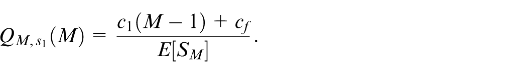
Scenario 1: Constant repair cost. Let $c_{1}$ be the unitary cost of repair.

The cost of a cycle is

C (τ) = c_{1} \min (M - 1, N (T)) + c_{a} I_{T} + c_{f} I_{M}

$N (T)$ accounts for the number of failures occurring until $T$ . $I_{T}$ , $I_{M}$ are the indicator variables of replacement at $T$ or on the $M$ failure, respectively.

The expected cost of a cycle is

\begin{matrix} E [C (τ)] = c_{1} E [\min (M - 1, N (T))] \\ + c_{a} P (I_{T} = 1) + c_{f} P (I_{M} = 1) \\ = c_{1} \sum_{k = 0}^{M - 2} kP (N (T) = k) \\ + c_{1} (M - 1) P (N (T) \geq M - 1) \\ + c_{a} P (S_{M} > T) + c_{f} P (S_{M} \leq T) \\ = c_{1} (M - 1 - \sum_{k = 0}^{M - 1} (M - 1 - k) P (N (T) = k)) \\ + c_{a} P (N (T) \leq M - 1) + c_{f} P (N (T) \geq M) \\ = c_{1} (M - 1 - \sum_{k = 0}^{M - 1} (M - 1 - k) P (N (T) = k)) \\ + c_{f} + (c_{a} - c_{f}) \sum_{k = 0}^{M - 1} P (N (T) = k) . \end{matrix}

(6)

The cost function in scenario 1 is

Q_{1} (T, M) = \frac{E [C (τ)]}{E [τ]}

with the mean cycle length, $E [τ]$ , and its corresponding expected cost, $E [C (τ)]$ , in equations (5) and (6), respectively.

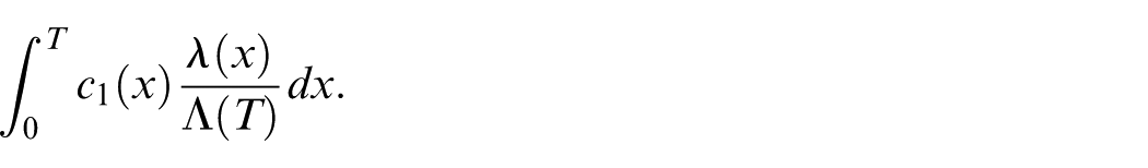
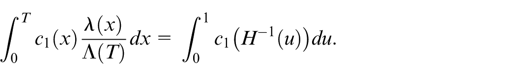
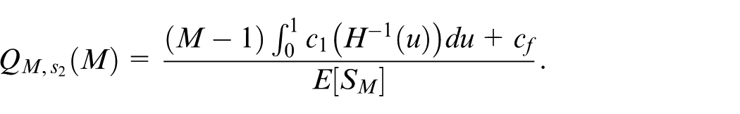
Scenario 2: The costs of repairs are time dependent, with $c_{1} (t)$ the unitary cost.

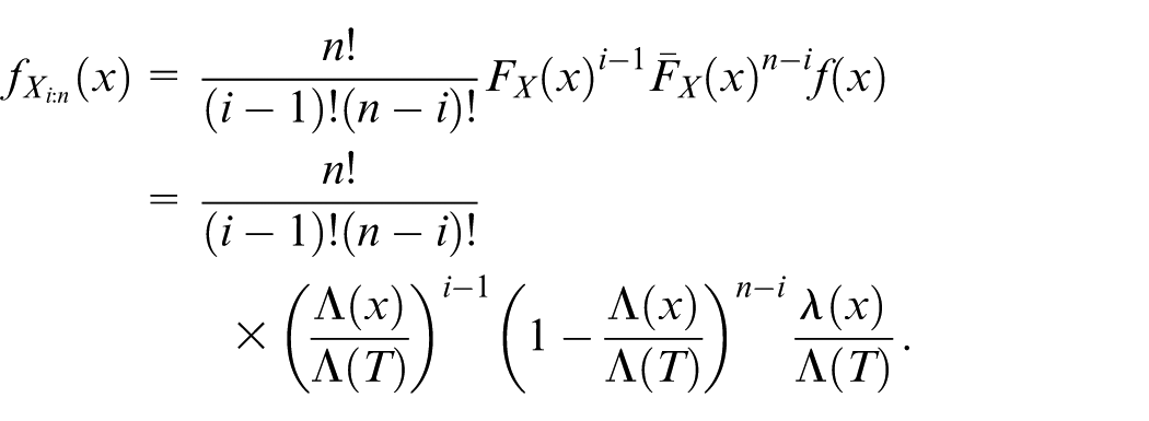
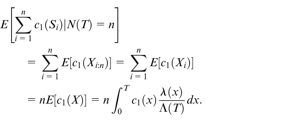
Assume that $n$ failures have happened in $(0, T)$ , then the order statistics $S_{1}, \dots, S_{n} | N (T) = n$ , representing the corresponding times until they occur, are independent random variables with probability density function $\frac{λ (x)}{Λ (T)}$ .

Moreover, consider a sample of size $n$ from a random variable $X$ , the density function of the $i$ th order statistics, $X_{i : n}$ , is:

For $0 \leq x \leq T$

\begin{matrix} f_{X_{i : n}} (x) = \frac{n!}{(i - 1)! (n - i)!} F_{X} {(x)}^{i - 1} {\bar{F}}_{X} {(x)}^{n - i} f (x) \\ = \frac{n!}{(i - 1)! (n - i)!} \\ \times {(\frac{Λ (x)}{Λ (T)})}^{i - 1} {(1 - \frac{Λ (x)}{Λ (T)})}^{n - i} \frac{λ (x)}{Λ (T)} . \end{matrix}

The renewal at $T$ occurs if there is not more than $M - 1$ failures in $[0, T]$ . The corresponding probability is $\sum_{n = 0}^{M - 1} P (N (T) = n)$ .

In addition, the times between consecutive failures, $X_{i}$ , are independent random variables with density function $\frac{λ (x)}{Λ (T)}$ .

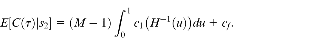
The mean cost incurred due to the repair of $n$ failures $(n \leq M - 1)$ :

\begin{matrix} E [\sum_{i = 1}^{n} c_{1} (S_{i}) | N (T) = n] \\ = \sum_{i = 1}^{n} E [c_{1} (X_{i : n})] = \sum_{i = 1}^{n} E [c_{1} (X_{i})] \\ = nE [c_{1} (X)] = n \int_{0}^{T} c_{1} (x) \frac{λ (x)}{Λ (T)} dx . \end{matrix}

The renewal after $M$ failures happens in case that $S_{M} \leq T$ . The corresponding probability is $\sum_{n = M}^{P} (N (T) = n)$ .

The mean cost derived from the repair of the first $M - 1$ failures is as follows:

\begin{matrix} E [\sum_{i = 1}^{M - 1} c (S_{i}) | N (T) = n] \\ = \sum_{i = 1}^{M - 1} E [c (X_{i : n})] = \int_{0}^{T} c_{1} (x) n \sum_{j = 0}^{M - 2} (\frac{n - 1}{j}) \times \\ ({(\frac{Λ (x)}{Λ (T)})}^{j} {(1 - \frac{Λ (x)}{Λ (T)})}^{n - 1 - j} \frac{λ (x)}{Λ (T)}) dx . \end{matrix}

Then, the mean cost of a renewal cycle:

\begin{matrix} E [C (τ)] = \sum_{n = 1}^{M - 1} nP (N (T) = n) \int_{0}^{T} c_{1} (x) \frac{λ (x)}{Λ (T)} dx \\ + \sum_{n = M}^{\infty} P (N (T) = n) \int_{0}^{T} c_{1} (x) n \sum_{j = 0}^{M - 2} (\frac{n - 1}{j}) \\ \times ({(\frac{Λ (x)}{Λ (T)})}^{j} {(1 - \frac{Λ (x)}{Λ (T)})}^{n - 1 - j} \frac{λ (x)}{Λ (T)}) dx \\ + c_{f} + (c_{a} - c_{f}) \sum_{k = 0}^{M - 1} P (N (T) = k) . \end{matrix}

(7)

The cost function in scenario 2:

Q_{2} (T, M) = \frac{E [C (τ)]}{E [τ]}

with $E [τ]$ and $E [C (τ)]$ in equations (5) and (7), respectively.

Observe that in case of $Z$ being a gamma random variable with scale parameter $α$ and shape parameter $β$ and $λ (t) = α r (t) e^{α \int_{0}^{t} r (u) du}$ , then the cost functions in scenarios 1 and 2 extend that in Lee and Cha²⁰ assuming $c_{a} = c_{f} = c_{r}$ and $c_{1} = c_{GPP}$ in the case of scenario 1 and $c_{1} (t) = c_{GPP}$ for scenario 2.

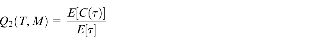
We aim at obtaining the optimum policy in both scenarios, that is, ( $T_{1}^{★}$ , $M_{1}^{★}$ ) minimizing $Q_{1} (T, M)$ and the corresponding ( $T_{2}^{★}$ , $M_{2}^{★}$ ) for $Q_{2} (T, M)$ .

Optimum number of repairs, $M$

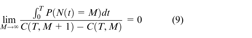
This section concerns the existence of an optimum $M^{★}$ minimizing $Q (T, M)$ , for a given $T$ , in scenarios 1 and 2. The first result provides the algorithm to obtain $M^{★}$ , simplifying programming tasks. The second serves to explore conditions under which there exists $M^{★}$ .

The notation below is used in what follows

C (T, M) = E [C (τ)] .

\begin{matrix} L (T, M) = C (T, M) \frac{\int_{0}^{T} P (N (t) = M) dt}{C (T, M + 1) - C (T, M)} \\ - \sum_{j = 0}^{M - 1} \int_{0}^{T} P (N (t) = j) dt . \end{matrix}

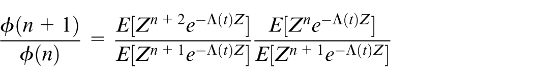
The following two results show the applicability of this model. First, Proposition 2 presents the strategy for computing the optimum $M$ , if it exists, when $T$ is given. It applies in both scenarios.

Proposition 2. Let $M^{*} = ar g_{M} \min Q (T, M)$ for a given $T > 0$ . If the function given next

\frac{\int_{0}^{T} P (N (t) = M) dt}{C (T, M + 1) - C (T, M)}

(8)

is decreasing in $M$ , and it verifies the following condition

\lim_{M \to \infty} \frac{\int_{0}^{T} P (N (t) = M) dt}{C (T, M + 1) - C (T, M)} = 0

(9)

then

M^{★} = \inf {M > 1 : L (T, M) < 0}

if $L (T, 1) > 0$ . If $L (T, 1) \leq 0$ , then $M^{*} = \infty$ .

The proof is in the Appendix A2.

The next theorem states sufficient conditions for the existence of an optimum $M$ in each scenario when the age replacement time is given. This information keeps the maintenance team aware of systems that need to be replaced earlier than planned.

Theorem 1. For a given age replacement time $T$ , the following results hold:

$a)$ Consider $Q_{1} (T, M)$ in scenario 1 with $c_{1} + c_{a} - c_{f} > 0$ . If either of the following conditions applies

$a_{1})$ Z is log concave and $λ (x)$ is increasing in $x$

$a_{2})$ Z is DFR, $λ (x)$ increasing in $x$ and $\frac{π (az)}{π (z)}$ is increasing in $z$ for $0 \leq a \leq 1$

then, there exists $M_{1}^{★} = ar g_{M} \min Q_{1} (T, M)$ .

$b)$ Consider $Q_{2} (T, M)$ in scenario 2 with $c_{a} = c_{f}$ . If $Z$ is IFR, $c_{1} (x)$ and $λ (x)$ are increasing in $x$ and $\frac{π (az)}{π (z)}$ is increasing in $z$ for $0 \leq a \leq 1$

then, there exists $M_{2}^{★} = ar g_{M} \min Q_{2} (T, M)$ .

The proof is in the Appendix A3.

Observe that if $Z$ is a gamma random variable with scale parameter $α$ and shapeparameter $\frac{β}{α}$ , then $Z$ is log concave for $β \geq α$ and DFR otherwise. Therefore, if $λ (x)$ is increasing in $x$ and $c_{1} + c_{a} - c_{f} > 0$ the conditions in $a_{1})$ apply for $β \geq α$ .

In addition, its density function verifies that $\frac{π (az)}{π (z)}$ is increasing in $z$ for $0 \leq a \leq 1$ and, hence, the conditions in $a_{1})$ hold. Thus, conditions in Theorem 1 for scenario 1 extend the results in Lee and Cha²⁰ (see Proposition 3).

Theorem 1 has interesting applications for maintainers when the age for replacement of a system, $T$ , is given. For example, this is useful when $T$ represents an amortization period. The corresponding bivariate policy takes into account the resulting reliability of the system after successive repairs. In the case of low quality repairs, the optimum policy may be an earlier replacement than indicated by the amortization period. Regarding the sufficient condition $c_{1} + c_{a} - c_{f} > 0$ , it seems to be a reasonable assumption when inspection is an expensive procedure. In addition, it trivially holds if $c_{a} \geq c_{f}$ . As mentioned previously, cases in which the system retains a residual value as a second-hand unit can imply that $c_{a} > c_{f}$ .

Comparison with univariate policies

In this section we present the classical univariate maintenance models, age replacement ( $T, \infty$ ) and replacement after a given number of failures ( $\infty, M$ ) assuming a MNHPP repair model. A comparison of the optimum cost derived from the three models gives light about the conditions under which the bivariate maintenance outperforms the other two.

Next we present the corresponding expressions of the cost function in scenarios 1 and 2.

Age replacement at T. M = $\infty$

The length of a cycle is $τ = T$ (non-random). The mean number of repairs is that of the mixture of non-homogeneous Poisson processes. In addition to the replacement cost, the cost derived from repairs until $T$ have to be considered. It follows that

E [τ] = T .

The cost of a cycle in scenarios 1 and 2 are respectively:

\begin{array}{l} E [C (τ) | s_{1}] = c_{1} E [N (T)] + c_{a} = c_{1} Λ (T) E [Z] + c_{a} . \\ E [C (τ) | s_{2}] = E [N (T)] \int_{0}^{T} c_{1} (x) \frac{λ (x)}{Λ (T)} d x + c_{a} \\ = Λ (T) E [Z] \int_{0}^{T} c_{1} (x) \frac{λ (x)}{Λ (T)} d x + c_{a} . \end{array}

with $Q_{T, s_{1}} (T)$ and $Q_{T, s_{2}} (T)$ being the corresponding cost functions in the two scenarios.

The optimum values minimizing $Q_{T, s_{1}} (T)$ and $Q_{T, s_{2}} (T)$ are denoted, respectively, by $T_{s_{1}}^{★}$ and $T_{s_{2}}^{★}$ .

Replacement after $M$ failures. $T = \infty$

The cycle verifies $τ = S_{M}$ and therefore it presents a random length, but the incurred cost is deterministic. It follows that

E [τ] = E [S_{M}] = \int_{0}^{\infty} x f_{S_{M}} (x) dx

with $f_{S_{M}} (x)$ in $(4)$ .

The length of a cycle can be alternatively expressed as follows:

\begin{matrix} E [τ] = E [S_{M}] = \int_{0}^{\infty} P (N (x) \leq M - 1) dx \\ = \sum_{k = 0}^{M - 1} \int_{0}^{\infty} P (N (x) = k) dx . \end{matrix}

The corresponding cost in scenario 1:

E [C (τ) | s_{1}] = (M - 1) c_{1} + c_{f} .

and the cost function

Q_{M, s_{1}} (M) = \frac{c_{1} (M - 1) + c_{f}}{E [S_{M}]} .

Regarding scenario 2 and $E [C (τ)]$ in equation (7), the expected cost of repairing a failure in $(0, T)$ is

\int_{0}^{T} c_{1} (x) \frac{λ (x)}{Λ (T)} dx .

Observe that $H (x) = \frac{Λ (x)}{Λ (T)}$ verifies that $dH (x) = \frac{λ (x)}{Λ (T)} dx$ . Considering $u = H (x)$ , it follows that

\int_{0}^{T} c_{1} (x) \frac{λ (x)}{Λ (T)} dx = \int_{0}^{1} c_{1} (H^{- 1} (u)) du .

Replacement on the $M$ failure when there is at least one repair $(M > 1)$ makes no sense if the expected cost of repair is infinite. The assumption below is required for the expected cost derived from repairs in a cycle to be finite in scenario 2:

\begin{matrix} \lim_{T \to \infty} \int_{0}^{T} c_{1} (x) \frac{λ (x)}{Λ (T)} dx \\ = \lim_{T \to \infty} \int_{0}^{1} c_{1} (H^{- 1} (u)) du = \lim_{T \to \infty} c_{1} (T) < \infty . \end{matrix}

and, thus, the expected cost of a cycle is

E [C (τ) | s_{2}] = (M - 1) \int_{0}^{1} c_{1} (H^{- 1} (u)) du + c_{f} .

The cost function in scenario 2:

Q_{M, s_{2}} (M) = \frac{(M - 1) \int_{0}^{1} c_{1} (H^{- 1} (u)) du + c_{f}}{E [S_{M}]} .

Now $M_{s_{1}}^{★}$ and $M_{s_{2}}^{★}$ denote the optimum number of failures previous to replacement minimizing $Q_{M, s_{1}} (M)$ and $Q_{M, s_{2}} (M)$ , respectively.

Aiming at giving additional insight about the advantages of a bivariate policy, $Q_{1} (T^{★}, M^{★})$ and $Q_{2} (T^{★}, M^{★})$ have to be compared with the univariate policies in both scenarios.

Numerical example

In this section we carry out a sensitivity analysis for both scenarios. We obtain and compare the corresponding optimum policies for the univariate and bivariate maintenance. Thus, we give light on how the decision variables depend on the parameters of the model, as well as about the conditions under which the cost of the univariate maintenance is no longer larger than that of the bivariate policy. It is important to note that the use of a bivariate strategy for replacement adds extra complexity for maintainers. Therefore, these results are useful to indicate when a simpler maintenance based on just one of the two can be applied.

The baseline hazard rate is given as follows

λ (t | s) = 0.01 s (t + 1) e^{\int_{0}^{t} 0.01 (u + 1) du}

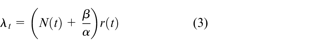
with $s > 0$ . If $s_{1} < s_{2}$ then $λ (t | s_{1}) < λ (t | s_{2})$ . Therefore, the parameter $s$ models the pace of the first failure. The higher $s$ , the more prone the system is to an early failure. This can be the result of different causes such as hidden defects, poor installation of the system, refurbished units used as spare parts, etc.

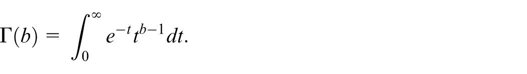
The mixing variable $Z$ follows a gamma distribution with density function:

π (z) = \frac{a^{b} z^{b - 1} e^{- az}}{Γ (b)}, z > 0 .

(10)

with $a > 0$ , $b > 0$ and $Γ (b)$ the Euler function:

Γ (b) = \int_{0}^{\infty} e^{- t} t^{b - 1} dt .

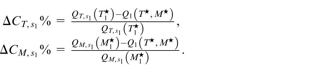
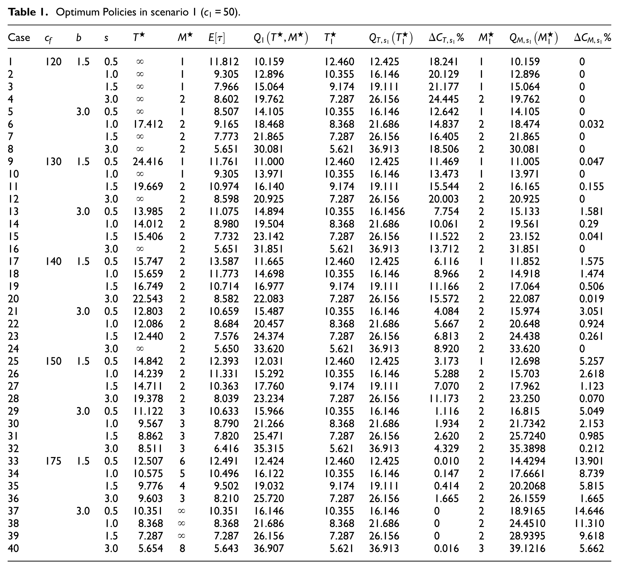
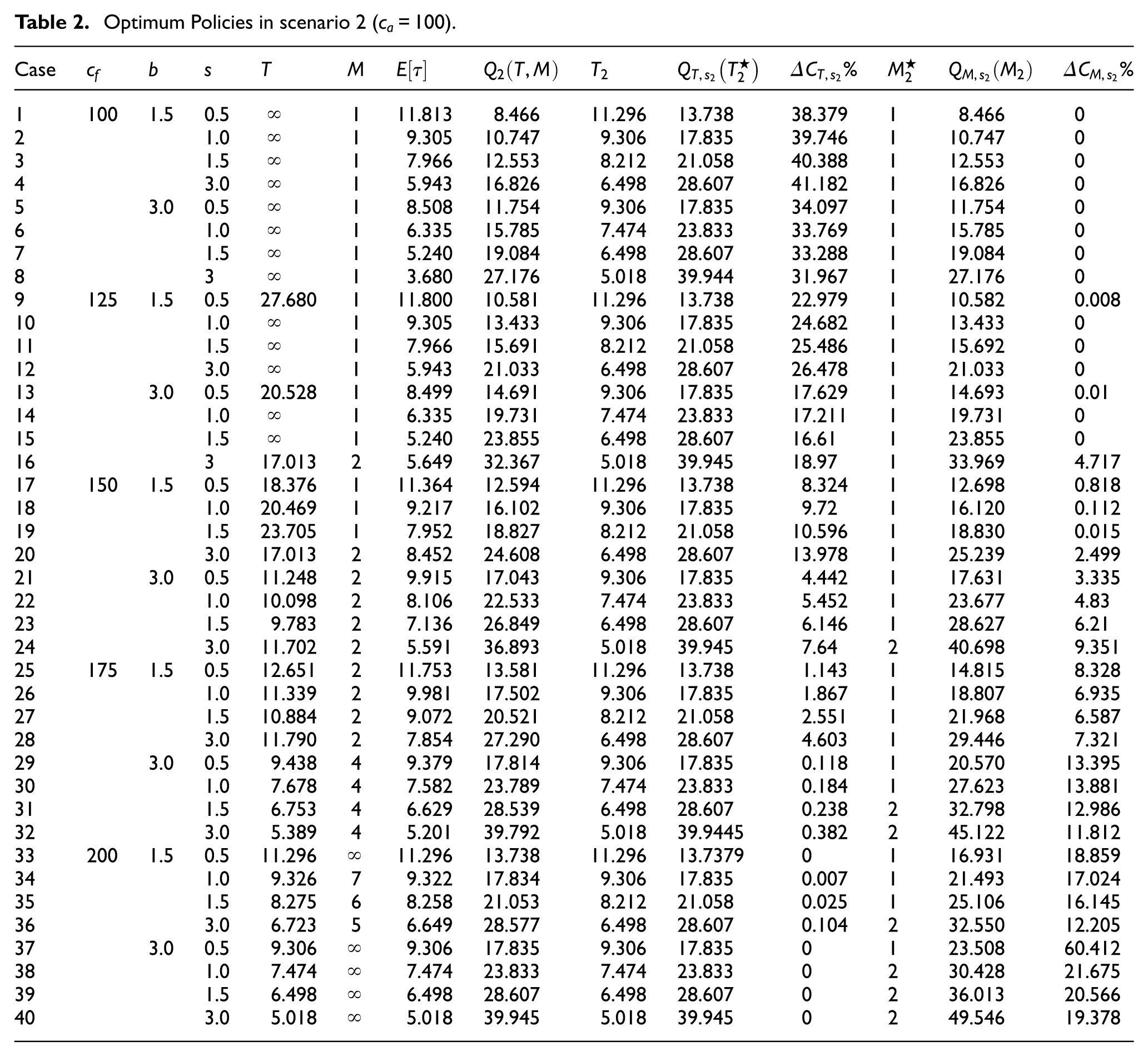
In what follows we will assume $a = 1$ and $c_{a} = 100$ . Tables 1 and 2 are obtained for $c_{1} = 50$ and $c_{1} (t) = 50 + 30 (1 - e^{- 0.1 t})$ corresponding to scenario 1 and 2, respectively. Both contain the optimum bivariate policy $(T^{★}, M^{★})$ , the optimum cost $Q_{i} (T^{★}, M^{★})$ as well as the univariate policies $T_{i}^{★}$ and $M_{i}^{★}$ along with the corresponding optimum costs, $Q_{T, s_{i}} (T_{i}^{★})$ and $Q_{M, s_{i}} (M_{i}^{★})$ , for $i = 1$ (scenario 1) in Table 1 and $i = 2$ (scenario 2) in Table 2. Table 1 also contains the following information for comparison purposes with the univariate policies:

\begin{matrix} Δ C_{T, s_{1}} % = \frac{Q_{T, s_{1}} (T_{1}^{★}) - Q_{1} (T^{★}, M^{★})}{Q_{T, s_{1}} (T_{1}^{★})}, \\ Δ C_{M, s_{1}} % = \frac{Q_{M, s_{1}} (M_{1}^{★}) - Q_{1} (T^{★}, M^{★})}{Q_{M, s_{1}} (M_{1}^{★})} . \end{matrix}

to compare with age replacement and replacement on the $M$ failure, respectively. Table 2 presents a similar study in scenario 2. The larger any of the two quantities above, the greater the advantage of the bivariate over its univariate competitors.

Table 1.

Optimum Policies in scenario 1 ( $c_{1} = 50$ ).

Case	$c_{f}$	$b$	$s$	$T^{★}$	$M^{★}$	$E [τ]$	$Q_{1} (T^{★}, M^{★})$	$T_{1}^{★}$	$Q_{T, s_{1}} (T_{1}^{★})$	$Δ C_{T, s_{1}} %$	$M_{1}^{★}$	$Q_{M, s_{1}} (M_{1}^{★})$	$Δ C_{M, s_{1}} %$
1	120	1.5	0.5	$\infty$	1	11.812	10.159	12.460	12.425	18.241	1	10.159	0
2			1.0	$\infty$	1	9.305	12.896	10.355	16.146	20.129	1	12.896	0
3			1.5	$\infty$	1	7.966	15.064	9.174	19.111	21.177	1	15.064	0
4			3.0	$\infty$	2	8.602	19.762	7.287	26.156	24.445	2	19.762	0
5		3.0	0.5	$\infty$	1	8.507	14.105	10.355	16.146	12.642	1	14.105	0
6			1.0	17.412	2	9.165	18.468	8.368	21.686	14.837	2	18.474	0.032
7			1.5	$\infty$	2	7.773	21.865	7.287	26.156	16.405	2	21.865	0
8			3.0	$\infty$	2	5.651	30.081	5.621	36.913	18.506	2	30.081	0
9	130	1.5	0.5	24.416	1	11.761	11.000	12.460	12.425	11.469	1	11.005	0.047
10			1.0	$\infty$	1	9.305	13.971	10.355	16.146	13.473	1	13.971	0
11			1.5	19.669	2	10.974	16.140	9.174	19.111	15.544	2	16.165	0.155
12			3.0	$\infty$	2	8.598	20.925	7.287	26.156	20.003	2	20.925	0
13		3.0	0.5	13.985	2	11.075	14.894	10.355	16.1456	7.754	2	15.133	1.581
14			1.0	14.012	2	8.980	19.504	8.368	21.686	10.061	2	19.561	0.29
15			1.5	15.406	2	7.732	23.142	7.287	26.156	11.522	2	23.152	0.041
16			3.0	$\infty$	2	5.651	31.851	5.621	36.913	13.712	2	31.851	0
17	140	1.5	0.5	15.747	2	13.587	11.665	12.460	12.425	6.116	1	11.852	1.575
18			1.0	15.659	2	11.773	14.698	10.355	16.146	8.966	2	14.918	1.474
19			1.5	16.749	2	10.714	16.977	9.174	19.111	11.166	2	17.064	0.506
20			3.0	22.543	2	8.582	22.083	7.287	26.156	15.572	2	22.087	0.019
21		3.0	0.5	12.803	2	10.659	15.487	10.355	16.146	4.084	2	15.974	3.051
22			1.0	12.086	2	8.684	20.457	8.368	21.686	5.667	2	20.648	0.924
23			1.5	12.440	2	7.576	24.374	7.287	26.156	6.813	2	24.438	0.261
24			3.0	$\infty$	2	5.650	33.620	5.621	36.913	8.920	2	33.620	0
25	150	1.5	0.5	14.842	2	12.393	12.031	12.460	12.425	3.173	1	12.698	5.257
26			1.0	14.239	2	11.331	15.292	10.355	16.146	5.288	2	15.703	2.618
27			1.5	14.711	2	10.363	17.760	9.174	19.111	7.070	2	17.962	1.123
28			3.0	19.378	2	8.039	23.234	7.287	26.156	11.173	2	23.250	0.070
29		3.0	0.5	11.122	3	10.633	15.966	10.355	16.146	1.116	2	16.815	5.049
30			1.0	9.567	3	8.790	21.266	8.368	21.686	1.934	2	21.7342	2.153
31			1.5	8.862	3	7.820	25.471	7.287	26.156	2.620	2	25.7240	0.985
32			3.0	8.511	3	6.416	35.315	5.621	36.913	4.329	2	35.3898	0.212
33	175	1.5	0.5	12.507	6	12.491	12.424	12.460	12.425	0.010	2	14.4294	13.901
34			1.0	10.575	5	10.496	16.122	10.355	16.146	0.147	2	17.6661	8.739
35			1.5	9.776	4	9.502	19.032	9.174	19.111	0.414	2	20.2068	5.815
36			3.0	9.603	3	8.210	25.720	7.287	26.156	1.665	2	26.1559	1.665
37		3.0	0.5	10.351	$\infty$	10.351	16.146	10.355	16.146	0	2	18.9165	14.646
38			1.0	8.368	$\infty$	8.368	21.686	8.368	21.686	0	2	24.4510	11.310
39			1.5	7.287	$\infty$	7.287	26.156	7.287	26.156	0	2	28.9395	9.618
40			3.0	5.654	8	5.643	36.907	5.621	36.913	0.016	3	39.1216	5.662

Table 2.

Optimum Policies in scenario 2 ( $c_{a} = 100$ ).

Case	$c_{f}$	$b$	$s$	$T^{★}$	$M^{★}$	$E [τ]$	$Q_{2} (T^{★}, M^{★})$	$T_{2}^{★}$	$Q_{T, s_{2}} (T_{2}^{★})$	$Δ C_{T, s_{2}} %$	$M_{2}^{★}$	$Q_{M, s_{2}} (M_{2}^{★})$	$Δ C_{M, s_{2}} %$
1	100	1.5	0.5	$\infty$	1	11.813	8.466	11.296	13.738	38.379	1	8.466	0
2			1.0	$\infty$	1	9.305	10.747	9.306	17.835	39.746	1	10.747	0
3			1.5	$\infty$	1	7.966	12.553	8.212	21.058	40.388	1	12.553	0
4			3.0	$\infty$	1	5.943	16.826	6.498	28.607	41.182	1	16.826	0
5		3.0	0.5	$\infty$	1	8.508	11.754	9.306	17.835	34.097	1	11.754	0
6			1.0	$\infty$	1	6.335	15.785	7.474	23.833	33.769	1	15.785	0
7			1.5	$\infty$	1	5.240	19.084	6.498	28.607	33.288	1	19.084	0
8			3	$\infty$	1	3.680	27.176	5.018	39.944	31.967	1	27.176	0
9	125	1.5	0.5	27.680	1	11.800	10.581	11.296	13.738	22.979	1	10.582	0.008
10			1.0	$\infty$	1	9.305	13.433	9.306	17.835	24.682	1	13.433	0
11			1.5	$\infty$	1	7.966	15.691	8.212	21.058	25.486	1	15.692	0
12			3.0	$\infty$	1	5.943	21.033	6.498	28.607	26.478	1	21.033	0
13		3.0	0.5	20.528	1	8.499	14.691	9.306	17.835	17.629	1	14.693	0.01
14			1.0	$\infty$	1	6.335	19.731	7.474	23.833	17.211	1	19.731	0
15			1.5	$\infty$	1	5.240	23.855	6.498	28.607	16.61	1	23.855	0
16			3	17.013	2	5.649	32.367	5.018	39.945	18.97	1	33.969	4.717
17	150	1.5	0.5	18.376	1	11.364	12.594	11.296	13.738	8.324	1	12.698	0.818
18			1.0	20.469	1	9.217	16.102	9.306	17.835	9.72	1	16.120	0.112
19			1.5	23.705	1	7.952	18.827	8.212	21.058	10.596	1	18.830	0.015
20			3.0	17.013	2	8.452	24.608	6.498	28.607	13.978	1	25.239	2.499
21		3.0	0.5	11.248	2	9.915	17.043	9.306	17.835	4.442	1	17.631	3.335
22			1.0	10.098	2	8.106	22.533	7.474	23.833	5.452	1	23.677	4.83
23			1.5	9.783	2	7.136	26.849	6.498	28.607	6.146	1	28.627	6.21
24			3.0	11.702	2	5.591	36.893	5.018	39.945	7.64	2	40.698	9.351
25	175	1.5	0.5	12.651	2	11.753	13.581	11.296	13.738	1.143	1	14.815	8.328
26			1.0	11.339	2	9.981	17.502	9.306	17.835	1.867	1	18.807	6.935
27			1.5	10.884	2	9.072	20.521	8.212	21.058	2.551	1	21.968	6.587
28			3.0	11.790	2	7.854	27.290	6.498	28.607	4.603	1	29.446	7.321
29		3.0	0.5	9.438	4	9.379	17.814	9.306	17.835	0.118	1	20.570	13.395
30			1.0	7.678	4	7.582	23.789	7.474	23.833	0.184	1	27.623	13.881
31			1.5	6.753	4	6.629	28.539	6.498	28.607	0.238	2	32.798	12.986
32			3.0	5.389	4	5.201	39.792	5.018	39.9445	0.382	2	45.122	11.812
33	200	1.5	0.5	11.296	$\infty$	11.296	13.738	11.296	13.7379	0	1	16.931	18.859
34			1.0	9.326	7	9.322	17.834	9.306	17.835	0.007	1	21.493	17.024
35			1.5	8.275	6	8.258	21.053	8.212	21.058	0.025	1	25.106	16.145
36			3.0	6.723	5	6.649	28.577	6.498	28.607	0.104	2	32.550	12.205
37		3.0	0.5	9.306	$\infty$	9.306	17.835	9.306	17.835	0	1	23.508	60.412
38			1.0	7.474	$\infty$	7.474	23.833	7.474	23.833	0	2	30.428	21.675
39			1.5	6.498	$\infty$	6.498	28.607	6.498	28.607	0	2	36.013	20.566
40			3.0	5.018	$\infty$	5.018	39.945	5.018	39.945	0	2	49.546	19.378

As $c_{f} / c_{a}$ increases, so does $M^{★}$ , but $T^{★}$ decreases. The higher cost of replacement on failure impels age replacement by reducing $T$ and increasing $M$ . Therefore, the relevance of the age replacement increases. Under this condition, the finite value of $T^{★}$ prevents the system from exceeding $M$ . Very large values of the ratio $c_{f} / c_{a}$ can result in $M^{★} = \infty$ (cases 37–39 in Table 1 and 37–40 in Table 2). On the contrary, as the ratio $c_{f} / c_{a}$ decreases, replacement based on the accumulated number of failures becomes more profitable than age replacement at $T$ , and therefore $T^{★} = \infty$ is observed more frequently. In fact, the cases considered where $c_{f} \approx c_{a}$ lead to $T^{★} = \infty$ .

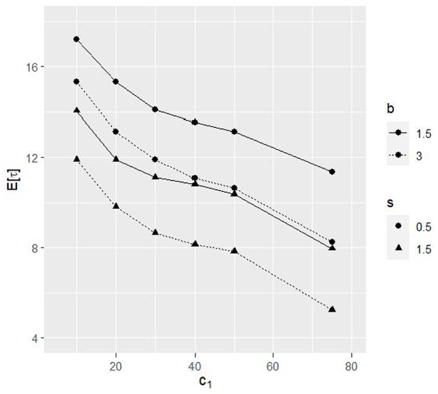
The higher $s$ , so is the initial failure rate of the system, leading to a decrease in expected length of a renewal cycle. The stochastic intensity of the failure process increases with $b$ and also leads to a reduction in $E [τ]$ . Therefore, the starting condition of a recycled component is critical when considering its use as a second-hand system. Poor repairs can also interfere with the purpose of extending the life of a system. Figure 1 illustrates this result, which must be considered when either recycled units are used as spares or the quality level of repairs drops. The comparison of the bivariate policy with the age replacement in scenarios 1 and 2 reveals that the cost reduction induced by the former decreases with $b$ . This means that the additional replacement on the $M$ failure is less advantageous the lower the quality of repairs is. This result is reversed in both scenarios when $s$ increases. Therefore, the bivariate policy is clearly superior to the age replacement in systems with low reliability when they start to work.

Figure 1.

Mean length of a renewal cycle under different values of $b$ , $s$ , and $c_{1}$ .

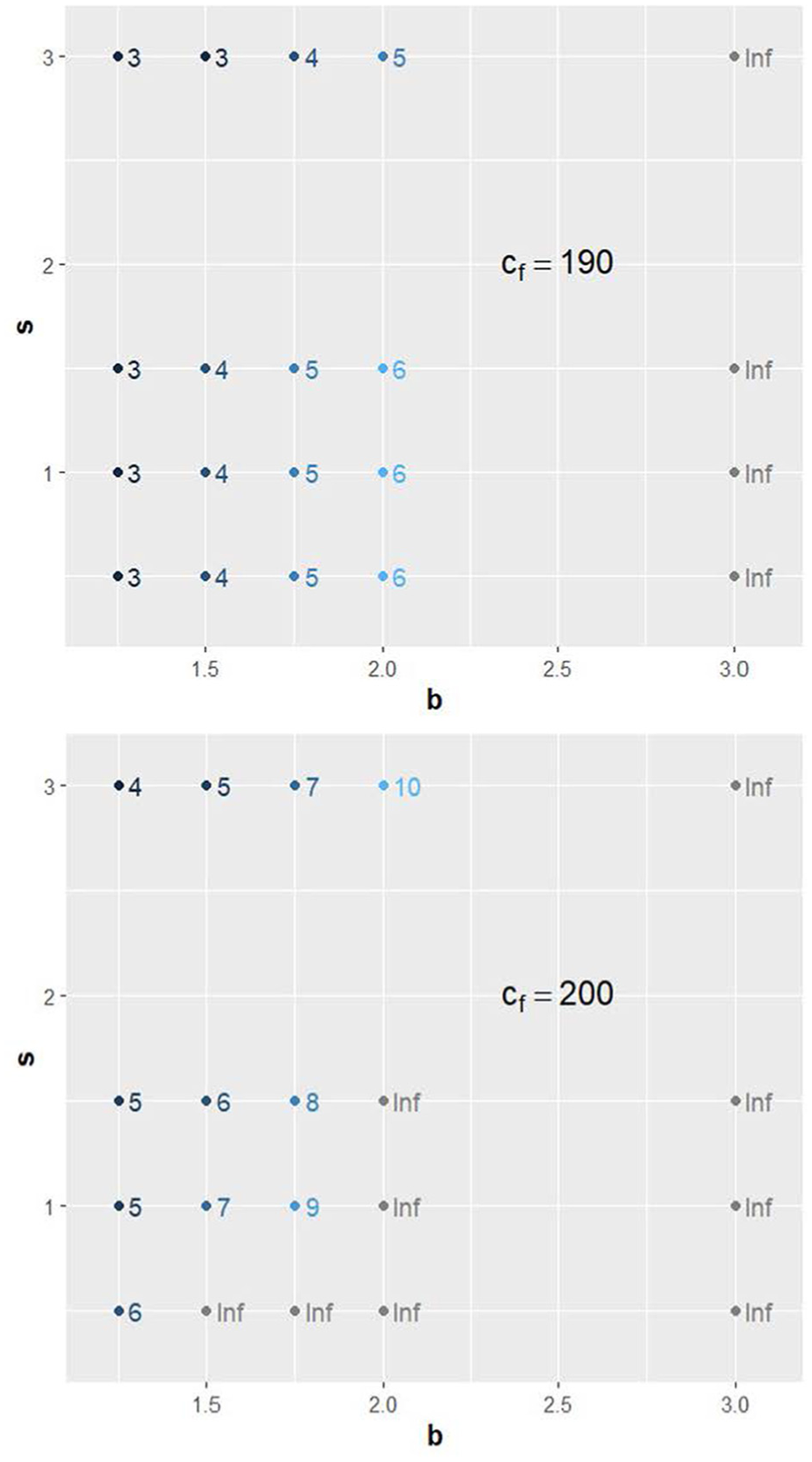
Notwithstanding that the bivariate policy outperforms the univariate maintenances in most cases, the sensitivity analysis also gives some insight into the conditions leading to either, $T^{★}$ or $M^{★}$ being infinite. If so, the optimum cost of the univariate policy is equal to that of the bivariate policy. Table 3 provides further information on the interaction effects of the three parameters, $c_{f}$ , $b$ , and $s$ in determining the optimum policy in scenario 2. If $b$ and $s$ are fixed, $M^{★} < \infty$ for $c_{f} = 190$ and $M^{★} = \infty$ for $c_{f} = 200$ (cases 5, 9, 13, 14, and 15). When $b$ is fixed, increasing $s$ leads to a decrease in $M^{★}$ , with some cases where $M^{★} = \infty$ drops to $M^{★} < \infty$ . This behavioris reversed when $s$ is fixed and $b$ increases. Figure 2 shows these results. Thus, the additional protection of the bivariate policy is more advantageous the lower the initial reliability of the system is. The bivariate policy tends to match an age replacement for large values of the parameter $b$ , which is the shape parameter of the mixing distribution $Z$ . According to equation (3), the larger $b$ , the worse the repair. In summary, a good maintenance is key for keeping systems operational. However, in case of a very low quality of repairs, the results do not show a clear gain in a more complex maintenance. An earlier age replacement might be sufficient.

Table 3.

Optimum Policies in scenario 2 ( $c_{a} = 100$ ).

	$c_{f} = 90$				$c_{f} = 200$
Case	$b$	$s$	$T^{★}$	$M^{★}$	$E [τ]$	$Q_{2} (T^{★}, M^{★})$	$T^{★}$	$M^{★}$	$E [τ]$	$Q_{2} (T^{★}, M^{★})$
1	1.25	0.5	12.261	3	12.062	12.864	11.863	6	11.857	12.887
2		1.0	10.519	3	10.202	16.526	9.937	5	9.903	16.595
3		1.5	9.633	3	9.216	19.364	8.874	5	8.826	19.494
4		3.0	8.510	3	7.797	25.861	7.517	4	7.308	26.203
5	1.50	0.5	11.443	4	11.387	13.729	11.296	$\infty$	11.296	13.738
6		1.0	9.570	4	9.474	17.802	9.326	7	9.322	17.834
7		1.5	8.570	4	8.441	20.991	8.275	6	8.258	21.053
8		3.0	7.726	3	7.097	28.392	6.723	5	6.649	28.577
9	1.75	0.5	10.893	5	10.876	14.520	10.843	$\infty$	10.843	14.522
10		1.0	8.983	5	8.952	18.964	8.886	9	8.885	18.976
11		1.5	7.954	5	7.910	22.462	7.823	8	7.820	22.488
12		3.0	6.609	4	6.416	30.643	6.194	7	6.182	30.733
13	2.00	0.5	10.471	6	10.466	15.255	10.455	$\infty$	10.455	15.256
14		1.0	8.560	6	8.550	20.042	8.524	$\infty$	8.524	20.046
15		1.5	7.529	6	7.514	23.823	7.474	$\infty$	7.474	23.833
16		3.0	6.043	5	5.974	32.711	5.858	10	5.857	32.750
17	3.00	0.5	9.307	$\infty$	9.307	17.836	9.306	$\infty$	9.306	17.835
18		1.0	7.474	$\infty$	7.474	23.833	7.474	$\infty$	7.474	23.833
19		1.5	6.498	$\infty$	6.498	28.607	6.498	$\infty$	6.498	28.607
20		3.0	5.018	$\infty$	5.018	39.945	5.018	$\infty$	5.018	39.945

Figure 2.

$M^{★}$ in scenario 2.

Conclusions

Replacing systems rather than repairing them when they fail or deteriorate, has been a common practice since the last decade of the last century. Nonetheless, this practice is no longer acceptable for sustainability reasons that lead to extend the use of components and systems by appropriate maintenance. This paper presents a bivariate maintenance policy based on both the age, $T$ , and the number of failures, $M$ . The combination of a deterministic and a random replacement generally gives additional protection to the system, since waiting for the age replacement at $T$ , may not be worthwhile in a system with a high frequency of failures. Therefore, a preventive maintenance after the $M$ failure, which occurs before the planned age replacement at $T$ , can be profitable from an economic point of view. However, poor quality maintenance can reduce the useful life of a system. There is unobserved heterogeneity between systems that seem to be identical due to differences in the quality of their maintenance. This variability is modeled by a frailty, $Z$ , which leads to a MNHPP in the failure process, which, in turn, is derived from a variety of minimal repairs carried out on failure. The value of $Z$ is specific to each system and remains constant throughout its life, but varies between systems depending on the quality of maintenance. This paper focuses on designing a maintenance policy that is valid for a heterogeneous population of systems. We analyze the consequences of low quality maintenance in the optimum policies under two scenarios with constant or time-dependent repair costs, respectively. The higher these costs, the earlier the system replacement implying a serious inconvenience to extend the time of use. We also provide sufficient conditions guaranteeing the existence of a finite $M$ in each of the two scenarios when $T$ is not a variable decision but a parameter in the model. This result, the maximum number of cost-effective repairs to be carried out, can serve as an indicator that an earlier replacement of the system, that is before the initial horizon at $T$ , iseconomically advantageous. Apart from the sensitivity analysis, the numerical study also addresses the comparison of the bivariate policy with the univariate ones, based only on the age $(M^{★} = \infty)$ or the number of cumulated failures $(T^{★} = \infty)$ . The initial reliability of a system when it starts to work is critical to determine the upcoming maintenance. The lower the initial reliability, the sooner the system will be replaced. Thus, the condition of a component that is to be used as a second-hand system is relevant to determine how it should be maintained. In fact, recycled units with low reliability levels can greatly benefit from the bivariate policy. The analysis reveals that some conditions can lead maintainers to use univariate maintenance policies, which are simpler to apply. Thus, $T^{★} = \infty$ is more likely to occur when the ratio $c_{f} / c_{a}$ is low, whereas $M^{★} = \infty$ tends to happen either when the former ratio is high or the mean quality of repairs decreases.

Footnotes

Appendix A1. Basics

Consider a random variable $X$

A random variable $X$ is

The following properties apply

$X$ is less or equal than $Y$ in

The following chain of implications concerning stochastic orders holds

Appendix A2. Auxiliary results

Let $S_{M}^{1}$ be a gamma random variable with shape parameter $M$ and scale parameter 1.

Lemma 1. $S_{M}^{1} \leq_{*} S_{M + 1}^{1}$ , with*=st, hr, rhr, lr.

Proof. It follows that

\frac{f_{S_{M + 1}^{1}} (x)}{f_{S_{M}^{1}} (x)} = \frac{\frac{1}{M!} x^{M} e^{- x}}{\frac{1}{(M - 1)!} x^{M - 1} e^{- x}} = \frac{x}{M}

is increasing in $x$ , thus $S_{M}^{1} \leq_{lr} S_{M + 1}^{1}$ which implies the st, hr and rhr stochastic orders.

Lemma 2. Let $f, g$ non null positive functions such that $\frac{f}{g}$ is decreasing. If $X \leq_{lr} Y$ , then

E [f (X)] E [g (Y)] - E [f (Y)] E [g (X)] \geq 0 .

Proof. If $\frac{f}{g}$ is decreasing, then $H (x, y) = f (x) g (y)$ verifies the condition for the bivariate characterization of likelihood ratio stochastic order in Shanthikumar and Yao²³ and the result follows.

Next, we define some auxiliary functions:

G (x) = \int_{x}^{\infty} \frac{1}{y} π (\frac{y}{Λ (T)}) dy .

For $M = 1, 2, \dots$ and $0 \leq u \leq 1$ :

\begin{matrix} A_{M} (u) = \int_{0}^{\infty} \frac{1}{z} F_{S_{M}^{1}} (Λ (T) zu) π (z) dz . \\ A_{M} (1) = \int_{0}^{\infty} \frac{1}{z} F_{S_{M}^{1}} (Λ (T) z) π (z) dz \\ = \int_{0}^{\infty} f_{S_{M}^{1}} (x) \int_{x}^{\infty} \frac{1}{y} π (\frac{y}{Λ (T)}) dydx \\ = E [G (S_{M}^{1})] . \end{matrix}

\begin{matrix} B_{M} (u) = \int_{0}^{\infty} F_{S_{M}^{1}} (Λ (T) zu) π (z) dz \\ = E [F_{S_{M}^{1}} (Λ (T) uZ)] . \\ B_{M} (1) = \int_{0}^{\infty} f_{S_{M}^{1}} (x) \int_{x}^{\infty} \frac{1}{Λ (T)} π (\frac{z}{Λ (T)}) dzdx \\ = E [{\bar{F}}_{Z} (\frac{S_{M}^{1}}{Λ (T)})] . \end{matrix}

The previous identity follows since

F_{S_{M}^{1}} (Λ (T) z) = P (S_{M}^{1} \leq Λ (T) z) = P (\frac{S_{M}^{1}}{Λ (T) z} \leq 1) .

Proof. $\frac{A_{M} (1)}{B_{M} (1)}$ is decreasing in $M$ if

(11)

\begin{matrix} (E [G (S_{M}^{1})] E [{\bar{F}}_{Z} (\frac{S_{M + 1}^{1}}{Λ (T)})] \\ - E [G (S_{M + 1}^{1})] E [{\bar{F}}_{Z} (\frac{S_{M}^{1}}{Λ (T)})]) \geq 0 . \end{matrix}

Next, we verify that Conditions in Lemma 2 hold:

Thus, the inequality in equation (11) is derived from Lemma 2.

Lemma 4. Let $X_{M}$ and $Y_{M}$ be random variables with probability density functions $f_{X_{M}}$ and $f_{Y_{M}}$ given, respectively, as follows

f_{X_{M}} (u) = \frac{1}{A_{M} (1)} \int_{0}^{\infty} \frac{1}{z} f_{\frac{S_{M}^{1}}{Λ (T) z}} (u) π (z) dz, 0 \leq u \leq 1

and

f_{Y_{M}} (u) = \frac{1}{B_{M} (1)} \int_{0}^{\infty} f_{\frac{S_{M}^{1}}{Λ (T) z}} (u) π (z) dz, 0 \leq u \leq 1

If $\frac{π (ax)}{π (x)}$ is an increasing function in $x$ for $0 \leq a \leq 1$ , then $X_{M} \leq_{st} X_{M + 1}$ and $Y_{M} \leq_{st} Y_{M + 1}$ .

Proof. $\frac{π (ax)}{π (x)}$ increasing in $x$ for $0 \leq a \leq 1$ , implies that $u Λ (T) Z \leq_{lr} Λ (T) Z$ which is one of the assumptions in Lemma 2.

Since the following equality applies

\begin{matrix} F_{X_{M}} (u) = \frac{A_{M} (u)}{A_{M} (1)} \\ = E [\frac{1}{Z} F_{S_{M}^{1}} (Λ (T) uZ)] / E [\frac{1}{Z} F_{S_{M}^{1}} (Λ (T) Z)] \end{matrix}

then, $F_{X_{M}} (u) \geq F_{X_{M + 1}} (u)$ is equivalent to

\begin{matrix} (E [\frac{1}{Z} F_{S_{M}^{1}} (Λ (T) uZ)] E [\frac{1}{Z} F_{S_{M + 1}^{1}} (Λ (T) Z)] \\ - E [\frac{1}{Z} F_{S_{M + 1}^{1}} (Λ (T) uZ)] E [\frac{1}{Z} F_{S_{M}^{1}} (Λ (T) Z)]) \geq 0 \end{matrix}

From Lemma 1 and the relation between the likelihood and usual stochastic orders, it follows that $\frac{\frac{1}{x} F_{S_{M}^{1}} (x)}{\frac{1}{x} F_{S_{M + 1}^{1}} (x)}$ is decreasing. Thus the previous inequality is derived from Lemma 2.

Likewise, $F_{Y_{M}} (u) = \frac{B_{M} (u)}{B_{M} (1)}$ , thus $F_{Y_{M}} (u) \geq F_{Y_{M + 1}} (u)$ iff

\begin{matrix} (E [F_{S_{M}^{1}} (Λ (T) uZ)] E [F_{S_{M + 1}^{1}} (Λ (T) Z)] \\ - E [F_{S_{M + 1}^{1}} (Λ (T) uZ)] E [F_{S_{M}^{1}} (Λ (T) Z)]) \geq 0 \end{matrix}

From Lemma 1, $\frac{F_{S_{M}^{1}} (x)}{F_{S_{M + 1}^{1}} (x)}$ is decreasing and conditions in Lemma 2 apply.

Note: Observe that $f_{\frac{S_{M}^{1}}{Λ (T) z}} (u) = f_{S_{M}^{1}} (Λ (T) zu) Λ (T) z$ .

Remark 1. The following alternative expression for $A_{M} (1)$ and $B_{M} (1)$ also apply:

\begin{matrix} A_{M} (1) = \int_{0}^{1} \int_{0}^{\infty} \frac{1}{z} f_{\frac{S_{M}^{1}}{Λ (T) z}} (u) π (z) dzdu \\ B_{M} (1) = \int_{0}^{1} \int_{0}^{\infty} f_{\frac{S_{M}^{1}}{Λ (T) z}} (u) π (z) dzdu \end{matrix}

Lemma 5. Let $X$ be a random variable, then:

The proof of this result can be found in Cuadras²⁴ and Joe.²⁵

Lemma 6. Let ${N_{1} (t) : t \geq 0}$ be a homogeneous Poisson process with failure rate $λ (t) = 1$ and $X$ a non negative random variable independent from the process and density function $f_{X}$ , it follows that

Proof. The preservation of the ageing classes given in (a) are well known results (see Grandell²⁶).

Case (b) is based on the following property stated in Shaked and Shanthikumar²⁷: If $A \leq_{lr} B$ , then $N_{1} (A) \leq_{lr} N_{1} (B)$ . Let $A = \frac{g (UT)}{g (T)} X$ and $B = X$ since the following identity applies

\frac{f_{A} (x)}{f_{B} (x)} = \frac{1}{f_{X} (x)} \int_{0}^{1} \frac{g (T)}{g (uT)} f_{X} (\frac{xg (T)}{g (uT)}) du

$f_{X} (\frac{xg (T)}{g (uT)}) / f_{X} (x)$ is decreasing in $x$ and so is $\frac{f_{A} (x)}{f_{B} (x)}$ , therefore the conclusion holds.

\begin{matrix} P (N_{1} (Λ (T) Z) = M) \\ = \int_{0}^{\infty} P (N_{1} (Λ (T) z) = M) π (z) dz \\ = \int_{0}^{\infty} e^{- Λ (T) z} \frac{{(Λ (T) z)}^{M}}{(M - 1)!} π (z) dz = P (N (T) = M) . \end{matrix}

Moreover, we have that $B_{M} (1) = P (N (T) \geq M)$ :

\begin{matrix} P (N (T) \geq M)) = P (N_{1} (Λ (T) Z) \geq M) \\ = \int_{0}^{\infty} P (S_{M}^{1} \leq Λ (T) z) π (z) dz \\ = \int_{0}^{\infty} π (z) \int_{0}^{Λ (T) z} f_{S_{M}^{1}} (x) dxdz \\ = \int_{0}^{\infty} f_{S_{M}^{1}} (x) \int_{x / Λ (T)}^{\infty} π (z) dzdx \\ = \int_{0}^{\infty} f_{S_{M}^{1}} (x) \int_{x}^{\infty} π (\frac{u}{Λ (T)}) \frac{1}{λ (T)} dudx \end{matrix}

The change $Λ (T) z = u$ leads to the last identity in the foregoing expression.

The identical distribution of $N (T)$ and $N_{1} (Λ (T) Z)$ is used along with Lemma 6 (a) to derive the ageing properties of $N (T)$ .

Remark 3. The use of Lemma 6 (b) is based on the following identity:

\begin{matrix} \int_{0}^{T} P (N (t) = M) dt \\ = \int_{0}^{T} P (N_{1} (\frac{Λ (t)}{Λ (T)} Λ (T) Z) = M) dt \\ = TP (N_{1} (\frac{Λ (UT)}{Λ (T)} Λ (T) Z) = M) \end{matrix}

where $U$ is a uniform random variable on the interval $[0, 1]$ independent from the Poisson process.

Lemma 7.

\int_{0}^{T} P (N (t) = M) dt = A_{M + 1} (1) E [\frac{1}{λ (H^{- 1} (X_{M + 1}))}]

$H^{- 1}$ is the inverse function of $H (t) = \frac{Λ (t)}{Λ (T)}, 0 \leq t \leq T$ .

Proof. $N (T) =^{st} N_{1} (Λ (T) Z)$ and the change $u = \frac{Λ (t)}{Λ (T)}$ lead to

\begin{matrix} \int_{0}^{T} P (N (t) = M) dt \\ = \int_{0}^{T} \int_{0}^{\infty} e^{- Λ (t) z} \frac{{(Λ (t) z)}^{M}}{M!} π (z) dzdt \\ = \int_{0}^{1} \frac{Λ (T)}{λ (H^{- 1} (u))} \int_{0}^{\infty} e^{- Λ (T) zu} \frac{{(Λ (T) zu)}^{M}}{M!} π (z) dzdu \\ = \int_{0}^{1} \frac{Λ (T)}{λ (H^{- 1} (u))} \int_{0}^{\infty} f_{S_{M + 1}^{1}} (Λ (T) zu) π (z) dzdu \\ = \int_{0}^{1} \frac{1}{λ (H^{- 1} (u))} \int_{0}^{\infty} \frac{1}{z} f_{\frac{S_{M + 1}^{1}}{Λ (T) z}} (u) π (z) dzdu . \end{matrix}

Calculations in the following Lemma involve the numerator of the cost function in scenario 2, denoted as C(T,M). Thus, $C (T, M) = E [C (τ)]$ with $E [C (τ)]$ in equation (7).

Lemma 8. If $c_{a} = c_{f}$ , it follows that

\begin{matrix} C (T, M + 1 \end{matrix}) - C (T, M) = \int_{0}^{1} c_{1} (H^{- 1} (x)) \int_{0}^{\infty} f_{\frac{S_{M}^{1}}{Λ (T) z}} (x) π (z) dzdx .

Proof:

\begin{matrix} C (T, M + 1) - C (T, M) \\ = MP (N (T) = M) \int_{0}^{T} c_{1} (x) \frac{λ (x)}{Λ (T)} dx \\ + \sum_{k = M + 1}^{\infty} \sum_{j = 0}^{M - 1} P (N (T) = k) k (\frac{k - 1}{j}) \times \\ \int_{0}^{T} c_{1} (x) {(\frac{Λ (x)}{Λ (T)})}^{j} {(1 - \frac{Λ (x)}{Λ (T)})}^{k - 1 - j} \frac{λ (x)}{Λ (T)} dx \\ - \sum_{k = M}^{\infty} \sum_{j = 0}^{M - 2} P (N (T) = k) k (\begin{matrix} k - 1 \\ j \end{matrix}) \times \\ \int_{0}^{T} c_{1} (x) {(\frac{Λ (x)}{Λ (T)})}^{j} {(1 - \frac{Λ (x)}{Λ (T)})}^{k - 1 - j} \frac{λ (x)}{Λ (T)} dx \\ \int_{0}^{T} c_{1} (x) {(\frac{Λ (x)}{Λ (T)})}^{j} {(1 - \frac{Λ (x)}{Λ (T)})}^{k - 1 - j} \frac{λ (x)}{Λ (T)} dx \\ + \sum_{k = M + 1}^{\infty} P (N (T) = k) k (\begin{matrix} k - 1 \\ M - 1 \end{matrix}) \int_{0}^{T} c_{1} (x) \times \\ ({(\frac{Λ (x)}{Λ (T)})}^{M - 1} {(1 - \frac{Λ (x)}{Λ (T)})}^{k - 1 - M + 1} \frac{λ (x)}{Λ (T)}) dx \\ - MP (N (T) = M) \sum_{j = 0}^{M - 2} (\frac{M - 1}{j}) \times \\ \int_{0}^{T} c_{1} (x) {(\frac{Λ (x)}{Λ (T)})}^{j} {(1 - \frac{Λ (x)}{Λ (T)})}^{M - 1 - j} \frac{λ (x)}{Λ (T)} dx \\ = \sum_{k = M}^{\infty} P (N (T) = k) k (\begin{matrix} k - 1 \\ M - 1 \end{matrix}) \int_{0}^{T} c_{1} (x) \times \\ ({(\frac{Λ (x)}{Λ (T)})}^{M - 1} {(1 - \frac{Λ (x)}{Λ (T)})}^{k - 1 - M + 1} \frac{λ (x)}{Λ (T)}) dx \\ = \int_{0}^{T} k c_{1} (x) \sum_{k = M}^{\infty} \int_{0}^{\infty} \frac{{(z Λ (T))}^{k}}{k!} e^{- z Λ (T)} π (z) \times \\ \frac{(k - 1)!}{(M - 1)! (k - M)!} {(\frac{Λ (x)}{Λ (T)})}^{M - 1} \times \\ {(1 - \frac{Λ (x)}{Λ (T)})}^{k - M} \frac{λ (x)}{Λ (T)} dzdx \\ = \int_{0}^{T} c_{1} (x) \int_{0}^{\infty} \frac{1}{(M - 1)!} {(\frac{Λ (x)}{Λ (T)})}^{M - 1} {(z Λ (T))}^{M} \times \\ (e^{- Λ (T) z} e^{Λ (T) z (1 - \frac{Λ (x)}{Λ (T)})} \frac{λ (x)}{Λ (T)} π (z)) dzdx \\ = \int_{0}^{T} c_{1} (x) \times \\ (\int_{0}^{\infty} \frac{z}{(M - 1)!} e^{- Λ (x) z} {(Λ (x) z)}^{M - 1} λ (x) π (z) dz) dx \end{matrix}

\begin{matrix} \int_{0}^{T} c_{1} (x) \int_{0}^{\infty} f_{S_{M}^{1}} (Λ (x) z) z λ (x) π (z) dzdx \\ \int_{0}^{1} c_{1} (H^{- 1} (u)) \int_{0}^{\infty} f_{S_{M}^{1}} (Λ (T) zu) z Λ (T) π (z) dzdu \\ \int_{0}^{1} c_{1} (H^{- 1} (u)) \int_{0}^{\infty} f_{\frac{S_{M}^{1}}{Λ (T) z}} (u) π (z) dzdu . \end{matrix}

The first expression in the last line is obtained after the change $u = \frac{Λ (x)}{Λ (T)} = H (x)$ .

Appendix A3. Existence of optimal policies in scenarios 1 and 2

Consider the following function

\begin{array}{l} L (T, M) = \\ C (T, M) \int_{0}^{T} \frac{P (N (t) = M) d t}{C (T, M + 1) - C (T, M)} \\ - \sum_{j = 0}^{M - 1} \int_{0}^{T} P (N (t) = j) d t . \end{array}

After basic calculations we obtain

(12)

Q (T, M + 1) \leq Q (T, M) \Leftrightarrow L (T, M) \geq 0, M = 1, 2, \dots

If the following condition applies

\lim_{M \to \infty} \frac{\int_{0}^{T} P (N (t) = M) dt}{C (T, M + 1) - C (T, M)} = 0

then

(13)

\lim_{M \to \infty} L (T, M) = - T < 0

$M \to \infty$ implies that only the age replacement at $T$ occurs and, from the univariate policies in Section 4, we have

\lim_{M \to \infty} C (T, M) = E (Z) Λ (T) \int_{0}^{T} c_{1} (t) \frac{λ (t)}{Λ (T)} dt + c_{a} < \infty .

In addition

\begin{matrix} L (T, M) - L (T, M + 1) = C (T, M + 1) \\ \times (\frac{\int_{0}^{T} (P (N (t) = M) dt}{C (T, M + 1) - C (T, M)} - \frac{\int_{0}^{T} (P (N (t) = M + 1) dt}{C (T, M + 2) - C (T, M + 1)}) \end{matrix}

and the next property follows:

$L (T, M)$ is decreasing in $M$ iff

(14)

\frac{\int_{0}^{T} P (N (t) = M) dt}{C (T, M + 1) - C (T, M)} is decreasing in M .

Proof of Proposition 2. From equation (14) $L (T, M)$ is decreasing in $M$ and, hence, $L (T, M) \leq L (T, 1)$ . In case that $L (T, 1) \leq 0$ , it follows that $L (T, M) \leq 0$ . From equation (12), $Q (T, M)$ is also decreasing in $M$ and the conclusion holds for $M^{*} = \infty$ .

Condition (9) leads to (13) and, if $L (T, 1) > 0$ , there exits $M$ such that $L (T, M) < 0$ . Let $M_{0} = \inf {M > 1 : L (T, M) < 0}$ . Since $L (T, M)$ is decreasing in $M$ , it follows that $L (T, M) \geq 0$ for $M = 1, \dots, M_{0}$ and $L (T, M) < 0$ for $M = M_{0}, M_{0} + 1, \dots$ . Then, from equation (12) it follows that $Q (T, M)$ is decreasing for $M = 1, \dots, M_{0}$ and increasing for $M = M_{0}, M_{0} + 1, \dots$ and the result holds with $M^{★} = M_{0}$ .

Proof of Theorem 1. $a)$ (Scenario 1). The expression of $C (T, M) = E [C (τ)]$ in equation (6) for scenario 1, leads to

\begin{matrix} C (T, M + 1) - C (T, M) \\ = c_{1} P (N (T) \geq M) + (c_{a} - c_{f}) P (N (T) = M) \\ = c_{1} P (N (T) \geq M + 1) + (c_{1} + c_{a} - c_{f}) P (N (T) = M) \end{matrix}

In addition, according to Remark 2, the following identity holds

P (N (T) \geq M + 1) = B_{M + 1} (1)

and, considering Lemma 7, the function in equation (8) can be also expressed as follows

(15)

\begin{matrix} \frac{\int_{0}^{T} P (N (t) = M) dt}{C (T, M + 1) - C (T, M)} \\ = \frac{A_{M + 1} (1)}{B_{M + 1} (1)} \frac{1}{(c_{1} + (c_{1} + c_{a} - c_{f}) \frac{P (N (T) = M)}{P (N (T) \geq M + 1)})} \\ \times E [\frac{1}{λ (H^{- 1} (X_{M + 1}))}] \end{matrix}

Next, we prove that if $a_{1})$ holds, then assumptions in Proposition 2 for scenario 1 apply. First, we obtain that equation (8) is decreasing in $M$ :

Hence,

\begin{matrix} E [\frac{1}{λ (H^{- 1} (X_{M + 1}))}] = \int_{0}^{1} \frac{1}{λ (H^{- 1} (u))} \times \\ (\int_{0}^{\infty} \frac{1}{A_{M + 1} (1)} \frac{1}{z} f_{\frac{S_{M + 1}^{1}}{Λ (T) z}} (u) π (z) dz) du \end{matrix}

is decreasing in $M$ since $λ (x)$ is assumed to be increasing under conditions $a_{1})$ and $a_{2})$ .

The following alternative expression for equation (8) leads to prove that this function is decreasing in $M$ under conditions $a_{2})$ in Theorem 1.

(16)

\begin{matrix} \frac{\int_{0}^{T} P (N (t) = M) dt}{C (T, M + 1) - C (T, M)} = \\ \frac{\int_{0}^{T} P (N (t) = M) dt}{P (N (T) = M)} \frac{1}{\frac{c_{1} P (N (T) \geq M)}{P (N (T) = M)} + c_{a} - c_{f}} . \end{matrix}

Under assumptions in $a_{2})$ , $\frac{π (az)}{π (z)}$ is increasing in $z$ for $0 \leq a \leq 1$ , then from Lemma 6 (b), it follows that $N_{1} (\frac{Λ (UT)}{Λ (T)} Λ (T) Z) \leq_{lr} N_{1} (Λ (T) Z)$ . Hence, $\frac{\int_{0}^{T} P (N (t) = M) dt}{P (N (T) = M)}$ is decreasing in $M$ and so is equation (16).

Next, we prove that the limiting condition (9) in Proposition 2 holds under assumptions in Theorem 1. Condition $c_{1} + c_{a} - c_{f} > 0$ , the stochastic order in $X_{M}$ and $\frac{1}{λ (x)}$ being a decreasing function apply under assumptions $a_{1})$ and $a_{2})$ , leading to the following inequality

\begin{matrix} \frac{\int_{0}^{T} P (N (t) = M)}{C (T, M + 1) - C (T, M)} \leq \frac{A_{M + 1} (1)}{B_{M + 1} (1)} \times \\ \frac{1}{(c_{1} + (c_{a} + c_{1} - c_{f}) \frac{P (N (T) = M)}{P (N (T) \geq M + 1)})} E [\frac{1}{λ (H^{- 1} (X_{1}))}] \\ \leq \frac{A_{M + 1} (1)}{c_{1} B_{M + 1} (1)} E [\frac{1}{λ (H^{- 1} (X_{1}))}] . \end{matrix}

In addition, according to Remark 1, it follows that

(17)

\frac{A_{M + 1} (1)}{B_{M} (1)} = \frac{\int_{0}^{1} \int_{0}^{\infty} \frac{1}{z} f_{\frac{S_{M + 1}^{1}}{Λ (T) z}} (u) π (z) dzdu}{\int_{0}^{1} \int_{0}^{\infty} f_{\frac{S_{M}^{1}}{Λ (T) z}} (u) π (z) dzdu} \leq \frac{Λ (T)}{M} .

The last inequality applies since

\begin{matrix} \int_{0}^{1} \int_{0}^{\infty} \frac{1}{z} f_{\frac{S_{M + 1}^{1}}{Λ (T) z}} (u) π (z) dzdu \\ = \int_{0}^{1} \int_{0}^{\infty} \frac{1}{z} f_{S_{M + 1}^{1}} (Λ (T) zu) Λ (T) z π (z) dzdu \\ = \int_{0}^{1} \int_{0}^{\infty} \frac{1}{z} \frac{1}{M!} e^{- Λ (T) zu} Λ {(T)}^{M} {(zu)}^{M} Λ (T) z π (z) dzdu \\ = \frac{Λ (T)}{M} \int_{0}^{1} \frac{1}{(M - 1)!} u \times \\ (\int_{0}^{\infty} e^{- Λ (T) zu} Λ {(T)}^{M - 1} {(zu)}^{M - 1} Λ (T) z π (z) dz) du \\ = \frac{Λ (T)}{M} \int_{0}^{1} u \int_{0}^{\infty} f_{\frac{S_{M}^{1}}{Λ (T) z}} (u) π (z) dzdu \\ \leq \frac{Λ (T)}{M} \int_{0}^{1} \int_{0}^{\infty} f_{\frac{S_{M}^{1}}{Λ (T) z}} (u) π (z) dzdu . \end{matrix}

In addition, the following function derived from Remark 2, can be expressed in the two next alternative ways that serve to prove that it is bounded either under conditions $a_{1})$ or $a_{2})$ .

(18)

\begin{matrix} \frac{B_{M} (1)}{B_{M + 1} (1)} \\ = 1 + \frac{P (N (T) = M)}{P (N (T) \geq M + 1)} \end{matrix}

(19)

\begin{matrix} = 1 + \frac{P (N (T) = M)}{P (N (T) = M + 1)} \frac{P (N (T) = M + 1)}{P (N (T) \geq M + 1)} \\ = \frac{P (N (T) \geq M)}{P (N (T) \geq M + 1)} . \end{matrix}

For $Z$ log concave (condition in $a_{1})$ ), $\frac{P (N (T) = M)}{P (N (T) = M + 1)}$ in equation (18) is decreasing in $M$ by Lemma 6 (a) and Remark 2.

For $Z$ DFR (condition in $a_{2})$ ), $N (T)$ is DFR by Lemma 6 (a) and Remark 2. Hence, $\frac{P (N (T) \geq M)}{P (N (T) \geq M + 1)}$ in equation (19) is decreasing in $M$ .

Therefore, applying equation (17), the product $\frac{A_{M + 1} (1)}{B_{M} (1)} \frac{B_{M} (1)}{B_{M + 1} (1)} = \frac{A_{M + 1} (1)}{B_{M + 1} (1)}$ tends to zero when $M$ tends to infinity and, thus, equation (9) applies. Therefore, conditions in Proposition 2 are fulfilled either $a_{1})$ or $a_{2})$ holds.

Proof of Theorem 1 $b)$ (Scenario 2). Now we consider scenario 2 with $c_{a} = c_{f}$ . Applying Lemma 8 we have

\begin{matrix} C (T, M + 1) - C (T, M) \\ = \int_{0}^{1} c_{1} (H^{- 1} (u)) \int_{0}^{\infty} f_{\frac{S_{M}^{1}}{Λ (T) z}} (u) π (z) dzdu \\ = B_{M} (1) E [c_{1} (H^{- 1} (Y_{M}))] . \end{matrix}

The previous identity and Lemma 7 lead to

(20)

\begin{matrix} \frac{\int_{0}^{T} P (N (t) = M)}{C (T, M + 1) - C (T, M)} \\ = \frac{A_{M + 1} (1)}{B_{M} (1)} \frac{E [\frac{1}{λ (H^{- 1} (X_{M + 1}))}]}{E [c_{1} (H^{- 1} (Y_{M}))]} . \end{matrix}

The following properties hold:

Therefore, under conditions given in $b)$ for scenario 2, the result in equation (14) follows.

Next, we prove that equation (9) also applies:

\begin{matrix} \int_{0}^{T} P (N (t) = M) dt \\ = \int_{0}^{T} \int_{0}^{\infty} e^{- Λ (t) z} \frac{{(Λ (t) z)}^{M}}{M!} π (z) dzdt \\ = \int_{0}^{1} \frac{1}{λ (H^{- 1} (u))} \int_{0}^{\infty} \frac{1}{z} f_{\frac{S_{M + 1}^{!}}{Λ (T) z}} (u) π (z) dzdu \end{matrix}

\begin{matrix} = A_{M + 1} (1) \int_{0}^{1} \frac{1}{λ (H^{- 1} (u))} \times \\ (\int_{0}^{\infty} \frac{1}{A_{M + 1} (1) z} f_{\frac{S_{M + 1}^{1}}{Λ (T) z}} (u) π (z) dz) du \\ \leq A_{M + 1} (1) \int_{0}^{1} \frac{1}{c_{1} (H^{- 1} (u)) λ (H^{- 1} (u))} \times \\ \int_{0}^{\infty} \frac{1}{A_{M + 1} (1) z} f_{\frac{S_{M + 1}^{1}}{Λ (T) z}} (u) π (z) dzdu \\ \times \int_{0}^{1} c_{1} (H^{- 1} (u)) \int_{0}^{\infty} \frac{1}{A_{M + 1} (1) z} f_{\frac{S_{M + 1}^{1}}{Λ (T) z}} (u) π (z) dzdu \\ = E [\frac{1}{c_{1} (H^{- 1} (X_{M})) λ (H^{- 1} (X_{M}))}] \times \\ \int_{0}^{1} c_{1} (H^{- 1} (u)) \int_{0}^{\infty} \frac{1}{z} f_{\frac{S_{M + 1}^{1}}{Λ (T) z}} (u) π (z) dzdu . \end{matrix}

Regarding the foregoing expressions, the last one in the first line is obtained after the change of variable $u = \frac{Λ (t)}{Λ (T)} = H (t)$ in the integral. Thus, $t = H^{- 1} (u)$ and $dt = \frac{λ (T)}{λ (t)} du$ .

The inequality in the third line follows applying Lemma 5 (b), since $c_{1} (x)$ is increasing and $\frac{1}{c_{1} (x) λ (x)}$ is decreasing. Furthermore

\begin{matrix} \int_{0}^{1} c_{1} (H^{- 1} (u)) \int_{0}^{\infty} \frac{1}{z} f_{\frac{S_{M + 1}^{1}}{Λ (T) z}} (u) π (z) dzdu \\ = \frac{Λ (T)}{M} \int_{0}^{1} c_{1} (H^{- 1} (u)) \times \\ (\int_{0}^{\infty} \frac{1}{(M - 1)!} Λ {(T)}^{M} {(zu)}^{M} e^{- Λ (T) zu} π (z) dz) du \\ \leq \frac{Λ (T)}{M} \int_{0}^{1} c_{1} (H^{- 1} (u)) \frac{1}{(M - 1)!} \times \\ (\int_{0}^{\infty} Λ {(T)}^{M - 1} z^{M - 1} u^{M - 1} e^{- Λ (T) zu} λ (T) z π (z) dz) du \\ = \frac{Λ (T)}{M} \int_{0}^{1} c_{1} (H^{- 1} (u)) (\int_{0}^{\infty} f_{\frac{S_{M}^{1}}{Λ (T) z}} (u) π (z) dz) du \\ = \frac{Λ (T)}{M} B_{M} (1) E [c_{1} (H^{- 1} (Y_{M}))] . \end{matrix}

Lemma 8 and the previous inequality lead to

\begin{matrix} \frac{\int_{0}^{T} P (N (t) = M)}{C (T, M + 1) - C (T, M)} \\ \leq \frac{Λ (T)}{M} E [\frac{1}{c_{1} (H^{- 1} (X_{M})) λ (H^{- 1} (X_{M}))}] \\ \leq \frac{Λ (T)}{M} E [\frac{1}{c_{1} (H^{- 1} (X_{1})) λ (H^{- 1} (X_{1}))}] . \end{matrix}

The last inequality follows since the assumption $c_{1} (x)$ and $λ (x)$ being increasing functions in Theorem 1 $b)$ , implies that $\frac{1}{c_{1} (H^{- 1} (u))}$ , $\frac{1}{λ (H^{- 1} (u))}$ are both decreasing. In addition, $X_{1} \leq_{st} X_{M}$ follows from the assumption $\frac{π (az)}{π (z)}$ , $0 \leq a \leq 1$ in Theorem 1 $b)$ and Lemma 4.

Hence, when $M$ tends to infinity, condition (9) holds. Thus, Proposition 2 applies under assumptions of scenario 2 in Theorem 1 $b)$ .

Acknowledgements

The authors thank the anonymous reviewers whose helpful comments significantly improved the final version of this paper.

ORCID iD

Francisco Germán Badía

Funding

The authors disclosed receipt of the following financial support for the research, authorship, and/or publication of this article: The work of F. G. Badía and M. D. Berrade is supported by the Spanish Ministry of Science and Innovation and the Spanish National Agency for Research under Projects PID2021-123737NB-I00 and PID2024-155364NB-I00, respectively. The work of H. Lee was supported by Hankuk University of Foreign Studies Research Fund of 2024 and the National Research Foundation of Korea (NRF) grant funded by the Korea government (MSIT) (No. RS-2023-00240817).

Declaration of conflicting interests

The authors declared no potential conflicts of interest with respect to the research, authorship, and/or publication of this article.

References

Cha

Finkelstein

Levitin

On the delayed worse-than-minimal repair model and its application to preventive replacement. IMA J Manag Math 2023; 34(1): 101–122.

Badía

Berrade

Cha

, et al. Optimal replacement policy under a general failure and repair model: minimal versus worse than old repair. Rel Eng Syst Saf 2018; 180: 362–372.

Wang

Dra

YASS

Cai

, et al. Advanced cold patching materials (CPMs) for asphalt pavement pothole rehabilitation: state of the art. J Clean Prod 2022; 366: Art. no. 133001.

Zouch

Yeung

Castanier

Optimizing road milling and resurfacing actions. Proc Inst Mech Eng O J Risk Reliab 2012; 226(O2): 156–168.

Khahro

SH.

Defects in flexible pavements: a relationship assessment of the defects of a low-cost pavement management system. Sustainability 2022; 14(24): 16475.

Huang

Bird

Heidrich

Development of a life cycle assessment tool for construction and maintenance of asphalt pavements. J Clean Prod 2009; 17(2): 283–296.

Nakagawa

Maintenance theory of reliability. Springer, 2005.

Mituzani

Zhao

Nakagawa

Age and periodic replacement policies with two failure modes in general replacement models. Rel Eng Syst Saf 2021; 214: Art. no. 107754.

Zong

Chai

Zhang

, et al. Optimal replacement policy for a deteriorating system with increasing repair times. Appl Math Model 2013; 37: 9768–9775.

10.

Zhao

Nakagawa

Optimization problems of replacement first or last in reliability theory. Eur J Oper Res 2012; 223: 141–149.

11.

Høyland

Rausand

System reliability theory. Models and statistical methods. Wiley, 1994.

12.

Safaei

Taghipour

An availability-constrained integrated maintenance–monitoring model for a system with failures following an NHPP. IEEE Trans Rel 2024; 73(2): 937–951.

13.

Brown

Liu

McIntyre

, et al. Reliability evaluation of repairable systems considering component heterogeneity using frailty model. Proc Inst Mech Eng O J Risk Reliab 2023; 237(4): 654–670.

14.

Liu

Wang

GJ.

Generalized polya-process-based reliability analysis for systems working under dynamic environment. IEEE Trans Rel 2024; 74(1): 2146–2156.

15.

Lee

Lan

Chien

, et al. Probabilistic and cost analyses of a renewable warranty with an inspection policy for a discrete operating item from a heterogeneous population. Appl Math Model 2021; 100: 138–151.

16.

Santos

ACD

Cavalcante

CAV

. A study on the economic and environmental viability of second-hand items in maintenance policies. Rel Eng Syst Saf 2022; 217: Art. no. 108133.

17.

Berrade

Calvo

Badía

FG.

Maintenance of systems with critical components. Prevention of early failures and wear-out. Comput Ind Eng 2023; 181: Art. no. 109291.

18.

Cha

Finkelstein

MS.

Point processes for reliability analysis. Springer, 2018.

19.

Lee

Cha

JH.

New stochastic models for preventive maintenance optimization. Eur J Oper Res 2016; 255: 80–90.

20.

Lee

Cha

JH.

A bivariate optimal replacement policy for a system subject to a generalized failure and repair process. Appl Stoch Model Bus 2019; 35: 637–650.

21.

Nakagawa

Finkelstein

A summary of maintenance policies for a finite interval. Rel Eng Syst Saf 2009; 94: 89–96.

22.

Ross

SM.

Stochastic processes. 2nd ed. Wiley, 2008.

23.

Shanthikumar

Yao

DD.

Bivariate characterization of some stochastic order relations. Adv Appl Probab 1991; 23: 642–659.

24.

Cuadras

CM.

On the covariance between functions. J Multivar Anal 2002; 81: 19–27.

25.

Joe

Multivariate models and dependence concepts. Chapman & Hall, 1997.

26.

Grandell

Mixed Poisson processes. Chapman & Hall, 1997.

27.

Shaked

Shanthikumar

JG.

Stochastic orders. Springer, 2007.

A mixed non-homogeneous Poisson process to model the quality of maintenance

Abstract

Keywords

Introduction

MNHPP repair model

Model building

Optimum number of repairs, M

Comparison with univariate policies

Age replacement at T. M = ∞

Replacement after M failures. T = ∞

Numerical example

Conclusions

Footnotes

Appendix A1. Basics

Appendix A2. Auxiliary results

Appendix A3. Existence of optimal policies in scenarios 1 and 2

Acknowledgements

ORCID iD

Funding

Declaration of conflicting interests

References

Optimum number of repairs, $M$

Age replacement at T. M = $\infty$

Replacement after $M$ failures. $T = \infty$