
Abstract
This paper proposes an improved adaptive density-based spatial clustering of applications with noise (DBSCAN) algorithm based on genetic algorithm and MapReduce parallel computing programming framework to improve the poor clustering effect and low efficiency of the DBSCAN algorithm, which due to experiential solving parameters. The size of Intensive Interval Threshold minPts and Scan Radius Eps would be rational planned by genetic algorithm iterative optimization, and it is secondary statute processing with the similarity and variability of the dataset and the efficient computing power of Hadoop Cluster. The data could be reasonable serialization, and the efficient adaptive parallel clustering could be achieved ultimately. Through the experimental results, it is shown that the proposed algorithm in this paper has higher clustering accuracy and execution efficiency than that of the comparison baselines. The trend will continue to grow with the increased volume of dataset. The improved algorithm provides a more accurate implementation method for the threshold of DBSCAN algorithm, and realizes the specific calculation process, which provides practice support for the realization of DBSCAN.
Keywords
Introduction
The density-based spatial clustering of applications with noise (DBSCAN) algorithm has always been the following two problems: for one thing, the threshold (minPts, Eps) is determined completely based on the experience, which directly leads to the low quality of the clustering results; and for the other, when processing the massive data, this algorithm is extremely inefficient. In the traditional algorithm, the method of setting the threshold parameters is directly set minPts = 4, the Eps value was determined by the observation, which led to the quality of follow-up clustering results cannot be guaranteed. Over the past years, a whole range of improvements were made for the problems of clustering quality. Lv et al. proposed a new concept core density reachable based on the influence space to address the problem of the DBSCAN algorithm performance that depends on two specified parameters, epsilon and minPts. 1 Lei et al. developed a new method named as P-DBSCAN to detect protein complexes in DPIN by using Pigeon-Inspired Optimization Algorithm to optimize the parameters e and minPts in DBSCAN. 2 Hou et al. presented a parameter-free algorithm based on the DSets (dominant sets) and DBSCAN algorithms to remove the dependence of clustering results on user-specified parameters. 3 Wang et al. introduced a density-based adaptive spatial clustering, according to the characteristics of the data structure and constantly changing the value of minPts to determine the optimal solution of Eps, to achieve the process of adaptive solution. 4 For dealing with time-consuming issues in large datasets, Kumar and Reddy proposed a novel graph-based index structure method groups that accelerates the neighbor search operations and also scalable for high-dimensional datasets, and experimental results show that the proposed method improves the speed of DBSCAN by a factor of about 1.5–2.2 on benchmark datasets. 5 Nasibov et al. proposed an algorithm DG2CEP that combines the density-based clustering algorithm DBSCAN with the data stream processing paradigm complex event processing to achieve continuous, on-line detection of clusters for higher frequency. 6 However, those improvements are used to adjust the two parameters minPts and Eps based on some method and some technique, simultaneously, to affect the clustering performance of the algorithm. When faced with large data environment problems, we should not only consider the impact of the adjustment of the two parameters (minPts and Eps) on the performance of the DBSCAN algorithm but also consider parallel processing problem in the DBSCAN algorithm.
The emergence of cloud computing and Hadoop platform makes it possible for the computation to be more efficient and time saving. He et al. presented a scalable DBSCAN algorithm using MapReduce to remove three major drawbacks in the existing parallel DBSCAN algorithms. 7 Kim et al. proposed a new density-based clustering algorithm which is robust to find clusters with varying densities and suitable for parallelizing the algorithm with MapReduce. 8 Yu et al. proposed an efficient distributed density-based clustering Cludoop algorithm for big data using Hadoop. 9 However, the above researches do not take into account the adjustment problem of the two parameters (minPts and Eps) on the performance of clustering algorithm. To solve this problem, this paper presents an improved DBSCAN algorithm based on genetic algorithm (GA-DBSCANMR). It adjusts minPts and Eps via the iteration and the fitness function in the genetic algorithm (GA) to improve the clustering accuracy of the DBSCAN algorithm. We utilize the Hadoop platform to parallelize the proposed algorithm, give the Map processing and Reduce process of the algorithm, which can reduce the running time of the algorithm and improve the clustering efficiency of the algorithm, and it is experimented with other similar algorithms.
Improvement of DBSCAN clustering algorithm
DBSCAN clustering algorithm
DBSCAN algorithm is able to find clusters of arbitrary shapes and filter the noise in the dataset. The related concepts are as follows 10 :
Core Point, Boundary Point, Noise Point: For the data object p, and p∈DS, if the point p is the center and Eps is the radius, while the number of points in NEps(p) exceeds the given minPts, then p is the Core Point; and if p is not the Core Point, but within a core area, then p is treated as the Boundary Point; else p is the Noise Point or Outlier Point.
Direct Density-reachable: Given a sample set DS, if p is in the neighborhood of q and q is the Core Point, then named from the object q to the object p is directly densely-reachable as shown in Figure 1(a).
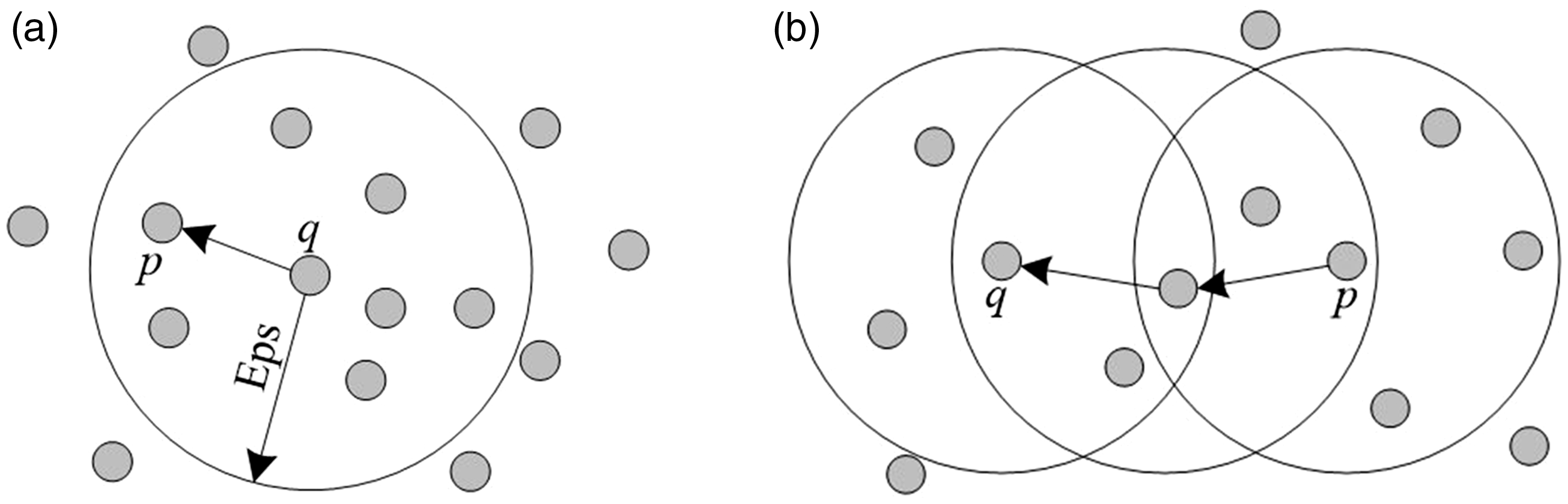
Density-reachable concept diagram: (a) Direct Density-reachable and (b) Density-reachable.
Density-reachable: Within a given sample set DS, if there is an object chain p1, p2, …, pn, where p1 = q, pn = p, and pi ∈ DS (1 ≤ i ≤ n), under the conditions of minPts and Eps, if from pi to pi+1 is Directed Density-reachable, then the object q from the object p is Density-reachable. Specific manifestations are shown in Figure 1(b), where from point q to point p is Density-reachable, while from point p to point q is not Density-reachable.
Density connection: If there is an object o ∈ DS, given that the objects p and q are Density-reachable from o at (minPts, Eps), then the density is connected from object p to q, and this density connection is symmetric. The concept diagram is shown in Figure 2, where points p and q are density connected with each other through the point o.
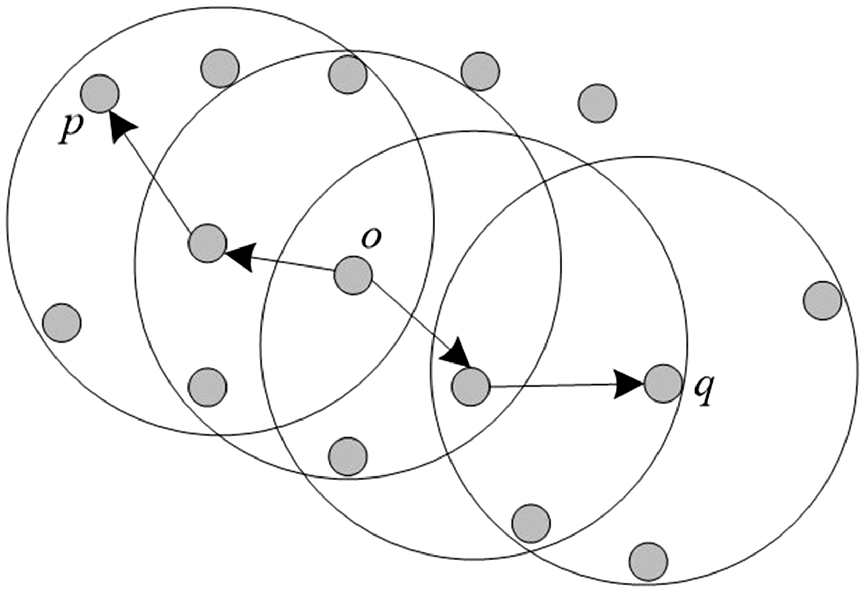
Density connection concept diagram.
Clusters: Starting from any of the Core Points, a cluster is formed from all object points whose density is reachable.
As mentioned above, the traditional algorithm is based entirely on the experience to set the values of the parameters minPts and Eps. This empirical approach leads directly to the credibility of the clustering results and the breadth of the application while consuming large amounts of time throughout the transverse process of the whole object data. It is simple for us to estimate that the implementation of the process of time complexity is O(n2). The traditional algorithm is extremely time consuming when the amount of the data is surging. In order to improve the quality of clustering and to combine with the MapReduce framework of Hadoop cluster, this paper introduces the GA to improve the traditional algorithm. The quality of clustering is improved and the problem of time consuming is solved as well. The improvement process is described below.
Design and improvement of GA-DBSCAN algorithm
Improvement GA method
In this paper, GA is used to improve the DBSCAN algorithm for determining the value of threshold minPts and Eps. The design of the improved algorithm mainly includes coding strategy, group setting, fitness function setting, and algorithm ending condition. For the coding problem, this paper uses the real coding method to directly use the solution space coding. Its advantage is based on specific problems that can be part or all of the components of the value of the constraints, with the original parameters of genetic operations, so that the optimal range is filled with the space that may exist in the optimal solution. It is easy to search for large space and is difficult to fall into the local extremum. It is possible to deal with complex variable constraints, multi-dimensional and high-precision numerical optimization problems, and complex optimization problems with unconventional constraints.
As for the group setting problem, the group size influences the final result of genetic optimization and the implementation efficiency of the GA. This paper sets the distribution range of the space occupied by the optimal solution in the whole problem space and then sets the initial population in this range. The method is as follows: establishing the dataset point distance matrix D. The matrix shows the distance
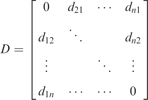
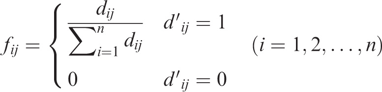
For the scan radius solution, we can compute the frequency of the distance overlap distance in the matrix D, set the interval with high overlap frequency to [a,b], and then revise D by the following formula
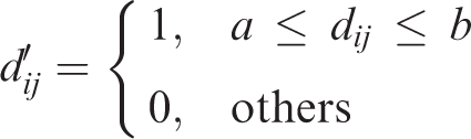
From this we can get the zero matrix of the Core Point to be selected. The initial group of the GA is the set of Core Points to be selected.
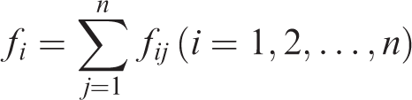
The fitness function of GA is not subject to continuous and differentiable, which is a non-negative result that can be calculated for input. Its design directly affects the performance of GA. The number of groups is set to n, according to the distance of the matrix D and the high overlap frequency interval relationship; the point distance fitness function is set as follows
Thus, the fitness of each selected Core Points in the initial population can be obtained by
The end condition of the algorithm is that when the number of algorithm iterations exceeds the maximum number of iterations K, the maximum fitness value in the group does not change. In this paper, we set K = 32, i.e., when the individual with the greatest fitness value continues to 32 generations without change, then we deem that the algorithm has been convergence and can be terminated. In the traditional methods, the iterative results of each algorithm are recorded in the register. With MapReduce, we can select the optimal solution with the largest fitness value directly from the list of Reduce results.
GA-DBSCAN algorithm
After several generations of evolution, if the optimal Core Point is still not found in the search process, it shows that the fathers selected in the previous generations cannot find the optimal point. The traditional GA, based on this method, conducts the continuous regeneration of the group, which leads to the joining of the individuals who are similar to their fathers. Therefore, the proportion of non-optimal individuals in the group is increased, resulting in genetic drift, and ultimately converge to the local optimal solution. Thus, the improvement of the traditional GA not only needs to take the group fitness, but also the dynamic adjustment category into consideration when selecting the fathers. The specific steps to improve the algorithm are as follows:
Define the adjustment coefficient α and the threshold θ, where α and θ are positive decimals, set the adjustment period K times, set the number of groups to be selected to n, the fitness function is f. Complete the following steps for the initial group:
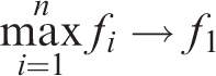
Estimate individual fitness of the initial group and perform the following operations
Back up the initial group so that it can be restored when it encounters the local minimum. The probability that the individual i is selected as the Core Point in the initial population is
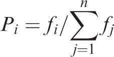
Use the probability Pi to select the Core Point and back up the selected individual.
3. Initialize the regenerative calculator I=0 and back up the selected Core Point according to the DBSCAN algorithm for clustering and the traditional GA for genetic operation. Stop if the optimal solution is found; otherwise I = I +1. 4. Remove the access to the Core Points in the current group and take the maximum fitness value for f2 in the rest group
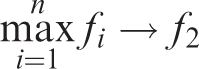
if
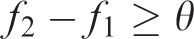
It means that the search process is still moving in the direction of optimization, replacing the individual in the reserved group with the individual in the current group,
if

It means that the convergence process is slow and may fall into the local optimum. At this time, the current population is replaced with the reserve group so that the population returns to the previous state of K generation and the determined minPts and Eps are replaced with the values of the previous population. The probability of selected individuals who are similar to or have been selected as the fathers in the former K generation is reduced. Namely

Go to (3).
5. Determine the number of individuals in the group and treat as the approximate value of the threshold minPts. The maximum dij of the dataset point distance matrix D by the group is assignment to Eps.
We can determine the Core Point and the corresponding threshold minPts and Eps using this algorithm. Time is mainly consumed in the iterative process of genetic algorithm. The time complexity of single iteration is O(n2), and the total time complexity is O(stn2) in the case of population number of s and iteration t times. In addition, the time complexity is higher than that in the K-means algorithm. However, this algorithm is able to effectively improve the precision of minPts and Eps, and to optimize the time-consuming problem of DBSCAN algorithm under the premise of increasing the precision of minPts and Eps.
GA-DBSCAN parallelization based on MapReduce
The GA-DBSCAN algorithm is not efficient when encountering a large amount of data. Therefore, we introduce a new GA-DBSCAN algorithm based on the MapReduce programming framework. Under the premise of ensuring the data partitioning is reasonable, the meshing and data binning technology of FPRBP algorithm 11 is used to exact division for original dataset to ensure that there is no overlapping area. On this basis, we can use Map and Reduce function to complete the parallelization of the algorithm, thus solving the problem of low efficiency of algorithm implementation. 12 Song et al. proposed a task distribution algorithm to optimize the energy consumption of MapReduce system. By adjusting the size of Map task and Reduce task dynamically, the size of the task processing data ensures task parallelism to reduce the overall energy consumption of MapReduce system. 13 Wang et al. proposed a MapReduce data equalization method based on the incremental partition strategy. On one hand, this method produces more Reducer number of fine-grained partition by JobTracker according to the global partition segment information screening part of the unallocated in the Map side. On the other hand, the corresponding fine-grained partition is assigned to each Reducer, which solves the problem of equalization after the data partitioning. 14 Xun et al. introduced the data placement strategy in MapReduce cluster environment and summarized and analyzed the research and development of the data placement strategy optimization method in the current MapReduce cluster environment. 15
Map process
Each data node (including Namenode and Datanode) performs the GA-DBSCAN clustering process on the assigned tasks. The intermediate clustering results are output in the form of key-value pairs <P, FCBCo> (<key, value>). P is the number of the data object and is unique across the entire dataset, so that the value of the key is value= (F, C, B, Co). It consists of four parts, where F is the partition number, and when the partition function FPRBP is executed (where the improved algorithm consumes a certain amount of time). C represents the cluster number. B indicates whether it is a boundary data object or not; Co indicates whether it is a core object or not. The process is shown in Figure 3.
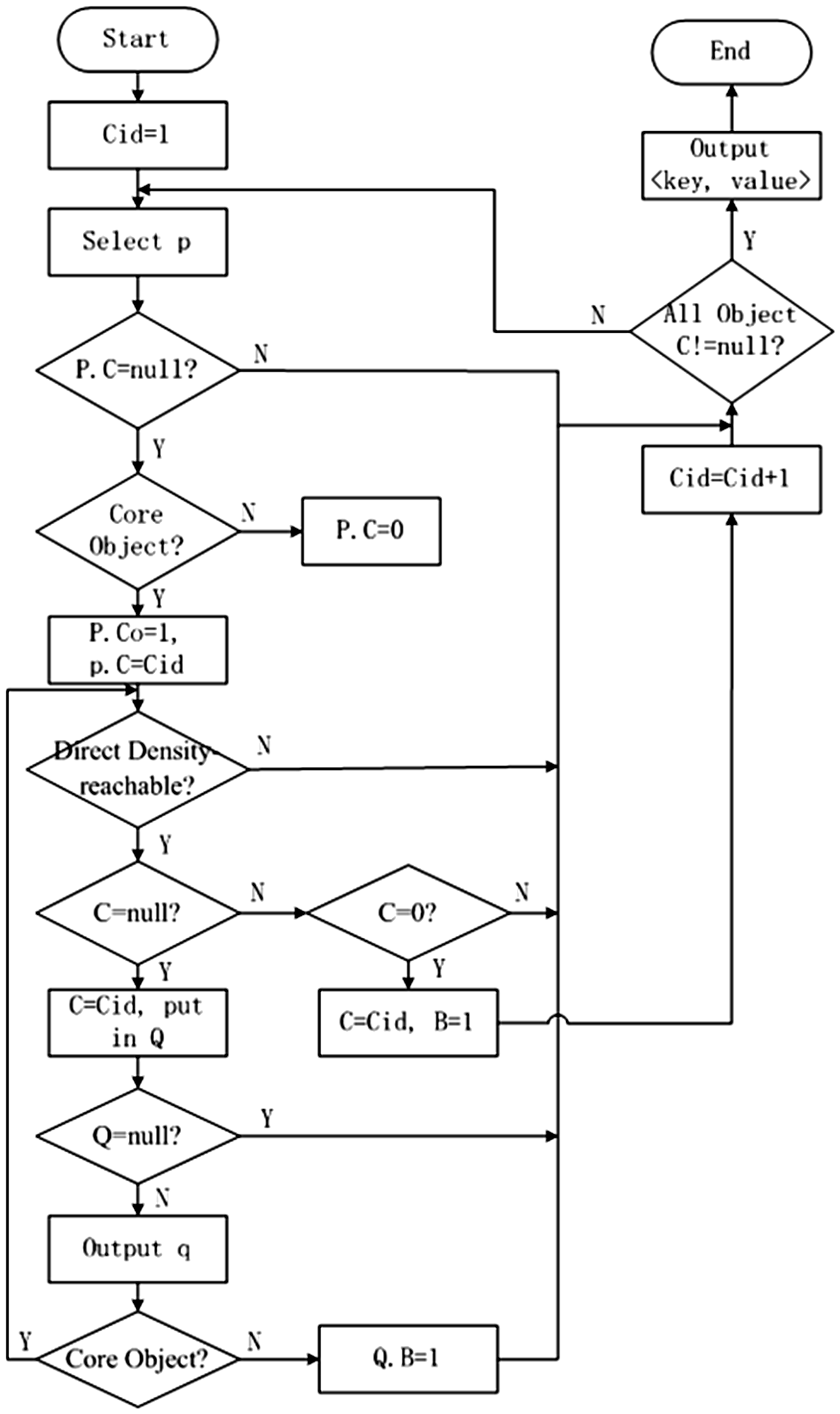
Map function flow.
Its formal description is as follows:
The initialized value of the variable Cid is set to 1, employ GA-DBSCAN algorithm to the dataset to determine minPts and Eps (at this time if the size of the dataset is small, cannot find significant difference in algorithm implementation efficiency between the improved algorithm and the original; when the amount of the data is surging, the effect will be obvious, which can be verified by the following experimental part); Select a data object p, and mark it with the value P, if cluster number of p is not null, jump to step (7); If p is the core object, the cluster number of p is assigned to Cid, else p is the Noise Point, the cluster number of p is assigned to 0; Traverses all the data objects that are directly accessible from p and determine that it is not a boundary object, assigns all object clusters whose number is not marked (cluster number is Null) to Cid, and is stored in queue Q. The object cluster number marked as noise (cluster number is 0) is assigned as Cid and is determined as a boundary object; If queue Q is empty, go to step (7), else remove queue header element q; If the data object q is the core object, running step (5), else it is determined that q is the boundary object value and the variable Cid value is incremented by 1; If all the data objects have a category tag, output the intermediate clustering result <key, value> to the Reduce process, end the Map process, else go to step (2).
Reduce process
Reduce processor receives the intermediate data <P, FCBCo> generated from the Map. Reduce process is divided into two parts. The specific algorithm flow is shown in Figure 4.
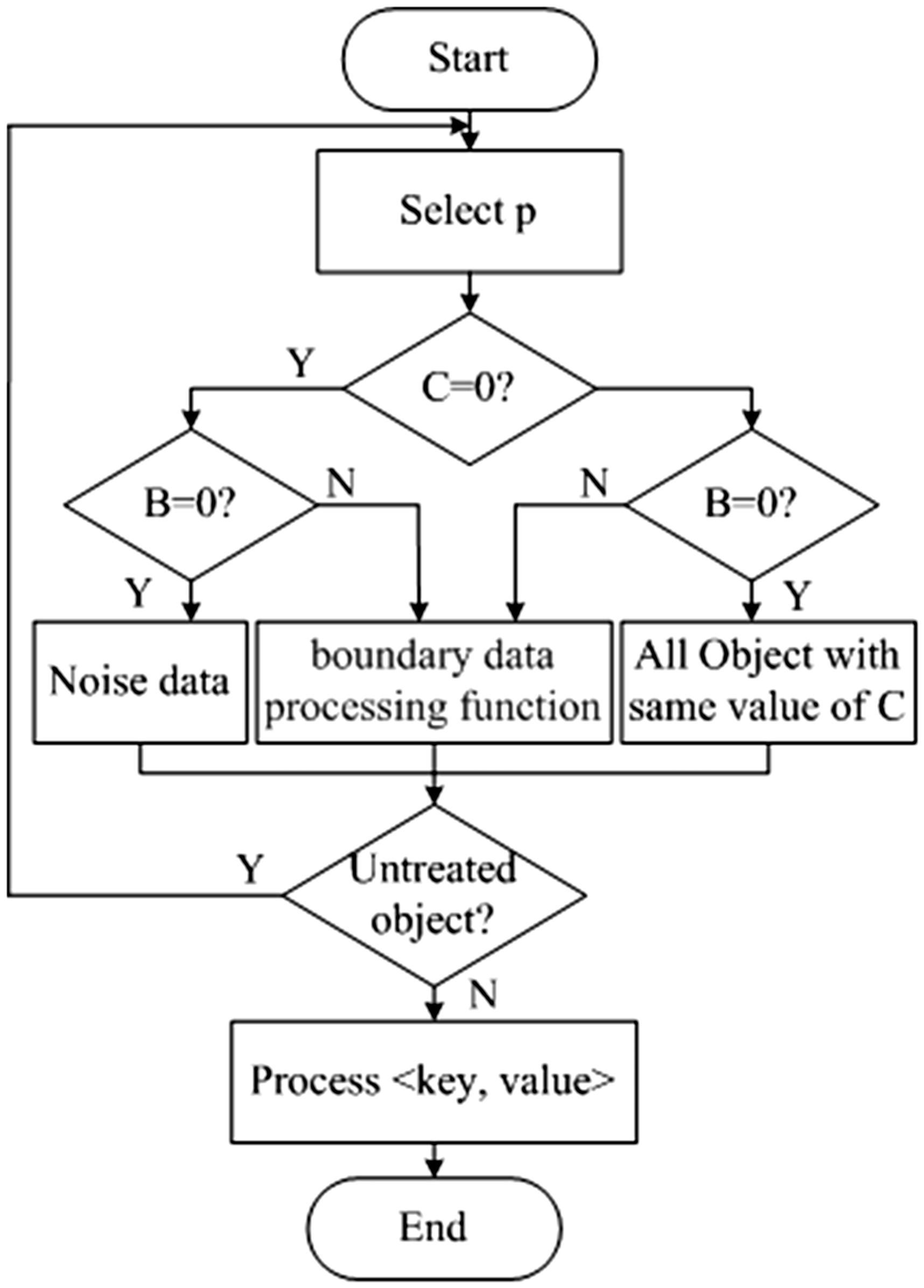
Reduce function flow.
Its formal description is as follows:
Select the data object p to determine whether it belongs to the noise set and boundary object; Do the following steps according to the value of p: If the data is marked as the noise and is not a boundary object, then it is marked as noise data; if neither the noise nor the data of the boundary object, then find all the data objects with the same cluster number; All the data marked as boundary objects then go to the boundary data processing function for further processing; If there is an unprocessed data object, go to step (1); According to the merging result of the boundary processing function, the cluster of the Clustering category in the whole dataset is re-numbered so as to obtain the unified cluster number, end the Reduce process, and output the final result <P, FCBCo>.
Analysis of the experimental results
The simulation experiment is carried out on the cluster of a host master with three slave node-computers. In addition, the master is the DELL PRECISION T1700 workstation. The configuration is as follows: quad-core, eight threads of Core i7-4770CPU, 16 GB memory, and SATA7200 r/min, hard drive with 1 TB capacity; the slave is equipped with the same Dell workstations of 8 GB memory, and 500 GB hard drive. The operating system is Ubuntu12.04, and all nodes were connected by the Gigabit Ethernet switch. The version of the Hadoop is 2.6.0.
The data are derived from the 30 GB Baidu Encyclopedia data obtained by the Nutch crawler, and the similarity of the data is processed. We select seven datasets with different number of data points, which were 3400, 9880, 14,886, 20,350, 24,650, 51,270, and 101,640, to carry out the clustering simulation experiments. The proposed algorithm is experimented for 10 times. And the experimental results are recorded. When the parent is selected, the proposed algorithm uses the fitness function to find the better value of adjustment parameter α and θ to set up. The relationship between them is as shown in Figure 5(a). After repeated experiments, we found that increasing the value of α and adjusting the θ in the iterative process can be used to avoid the appearance the local optimal solution of minPts and Eps. The relationship between the parameter θ and the accuracy rate of minPts, summarized from the experimental data, is given in Figure 5(b). The accuracy of the algorithm execution will be higher under the premise of the optimization process. But the accuracy rate is not continuous with the increase of θ when θ increases to a certain extent. As θ continues to increase, the accuracy decreases linearly. Therefore, through the coding strategy, the fitness function setting and the algorithm ending condition of GA in the proposed algorithm, the effective adjustment parameter α and θ can be determined better, so as to ensure the accuracy of the clustering algorithm.
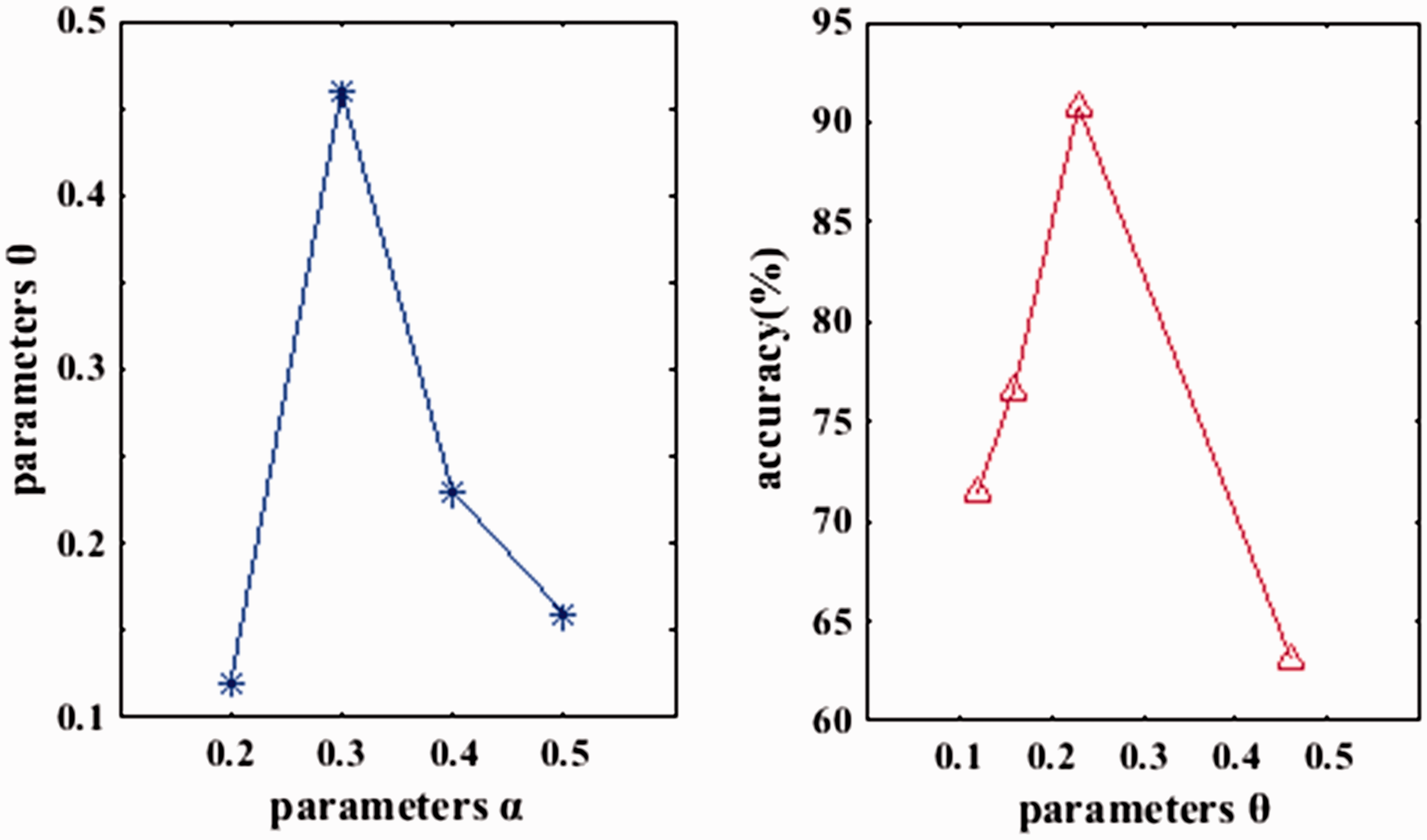
The relationship between the parameter and the correct rate: (a) Relationship between α and θ and (b) Relationship between θ and minPts.
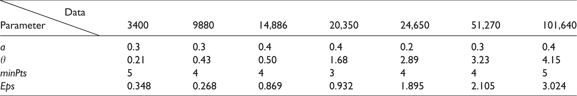
We choose the original DBSCAN algorithm, GA-DBSCAN algorithm, GRIDBSCAN method, 16 and DBSCAN-MR-N method 17 as comparison baselines of the proposed GA-DBSCAN algorithm based on the MapReduce programming framework (abbreviated as GA-DBSCANMR). Those clustering methods are experimented in the selected seven datasets. The values of α and θ of each method in experiments are recorded in Table 1. The accuracy rate of the corresponding clustering results of each method is exhibited in Table 2. We can observe that the clustering efficiency of the GA-DBSCANMR algorithm is obviously higher than that of other methods with the increasing number of the data points.
Parameter adaptation value.
Accuracy of the algorithm execution (%).
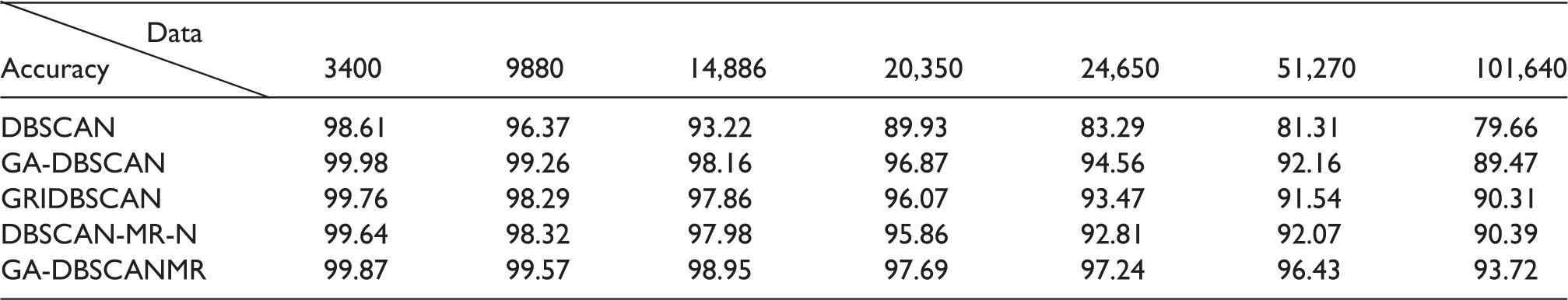
DBSCAN: density-based spatial clustering of applications with noise.
The running time of each method on each data point set in the above experiments is recorded and their average running time is compared when the parameter α is set to 0.3 and θ is set to 0.21 (Figure 6). We can see that the GA-DBSCANMR algorithm has lower running time than other methods when the number of the data points is less than 20,000, but the advantage is not obvious. This is because of the implementation of the partition function FPRBP and the assignment of tasks to the node Time, which will consume a certain amount of time. When the amount of the data increased to the next order of magnitude, the role of MapReduce is highlighted, and with the increasing amount of the data, standalone DBSCAN algorithm execution time showed a linear growth trend. So, when the number of data points increases gradually, the running time of GA-DBSCANMR algorithm is obviously less than that of other algorithms. This proves that the GA-DBSCANMR algorithm is suitable for processing large amounts of data points. And the clustering effect of the GA-DBSCANMR algorithm is shown in Figure 7.
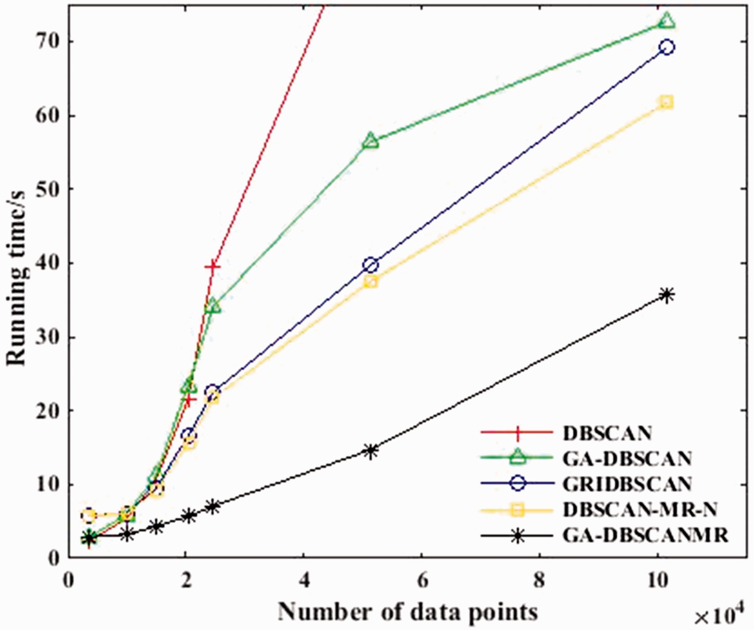
Contrast map with Running time/s.
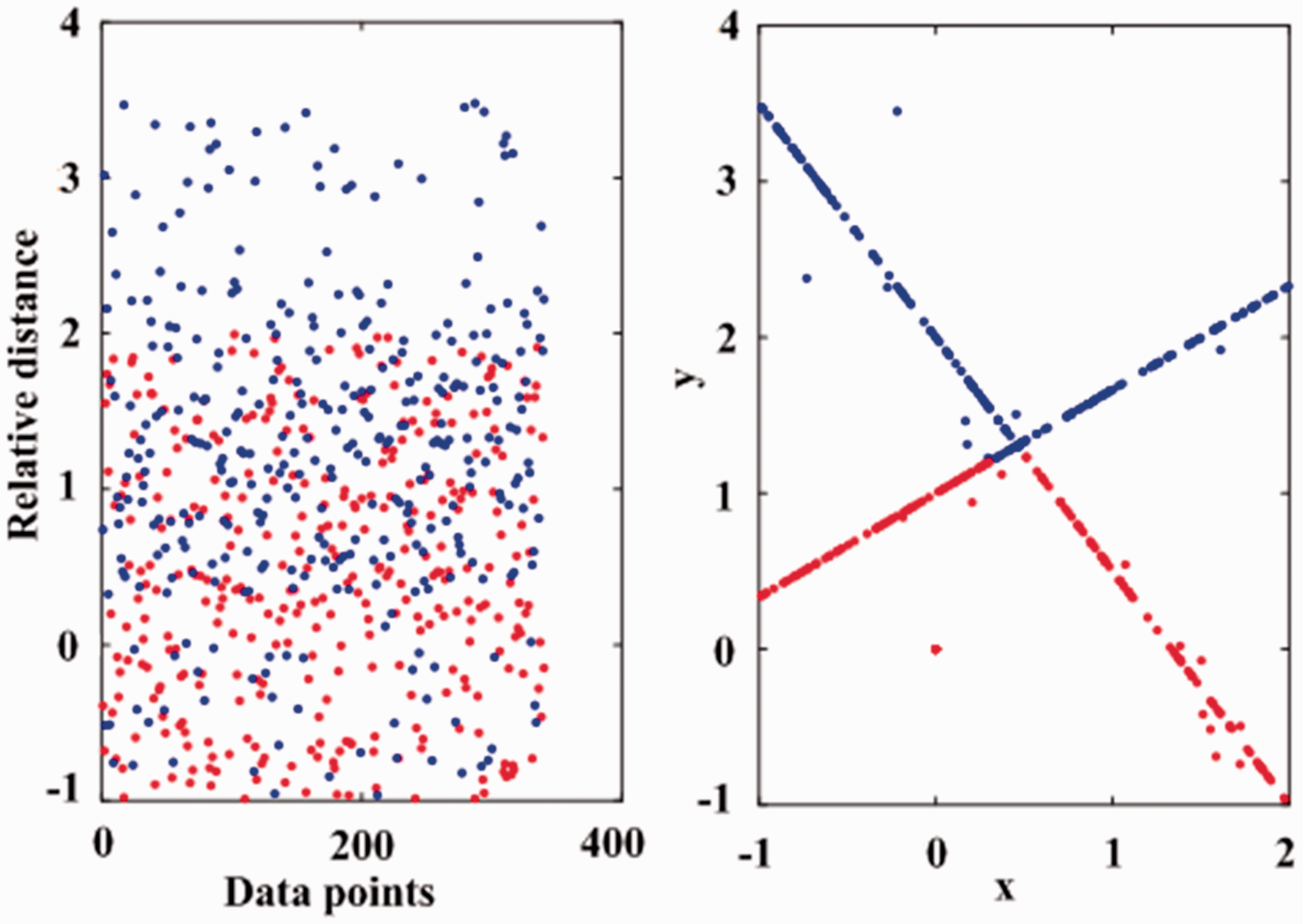
GA-DBSCANMR algorithm clustering results.
Conclusion
In this paper, a new DBSCAN algorithm is proposed, and the algorithm is improved using the genetic algorithm and the MapReduce programming framework. The original algorithm and the improved algorithm are compared experimentally. The following conclusions are drawn from the research process and the experimental results: (1) Based on the combination of GA, the approximation value of minPts and Eps can be determined automatically, instead of relying on experience to set the threshold, and thus greatly improve the accuracy of clustering. (2) In order to solve the problem that the algorithm is time consuming, the MapReduce programming framework is combined with the large dataset to the Hadoop Cluster. The experimental results show that the improved algorithm still maintains high efficiency when the data volume increases.
Through the improvement of the classical DBSCAN algorithm, the efficiency of the algorithm is greatly improved, and the accuracy of the algorithm is improved as well. However, it is still time consuming to improve the algorithm for high-dimensional data. Future work will focus on the high-dimensional datasets, so that the algorithm is able to achieve a wide range of applications.
Footnotes
Acknowledgment
The authors would like to thank the editor and all the referees for their useful comments and contributions for the improvement of this paper.
Declaration of conflicting interests
The author(s) declared no potential conflicts of interest with respect to the research, authorship, and/or publication of this article.
Funding
Acknowledgements
The author(s) disclosed receipt of the following financial support for the research, authorship, and/or publication of this article: This work was supported by the Natural Science Foundation of Jilin Province (20150101054JC), Postdoctoral Research Fund of Jilin Province (40301919) and the Key Program for Science and Technology Development of Jilin Province (20150204036GX).