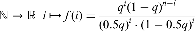
Lower bound on the information-loss incurred by compressing a depth-2 feed-forward layer of transformer into a single fully connected layer

Abstract

We consider the compression of a depth-2 feed-forward layer of Transformer into a single fully connected layer. To model this, we take a binary vector with independent entries as input. We define the event $A$ to be that for two disjoint subsets of size $k$ of the $0, 1$ entries of the vector, all entries of at least one of the subsets are equal to $1$ . This represents the information of two layers of a feed-forward layer. We study the approximation of the event $A$ by applying a linear functional to the binary vector, followed by a Heaviside (threshold) function. We establish an explicit lower bound on the relative error of any such approximation, valid for all choices of linear functionals. Notably, this lower bound approaches $1 / 16$ as $k$ becomes large. This result provides a theoretical explanation for the well-known heuristic that sparse Transformers, although requiring more parameters, achieve better performance. If it were possible to approximate $A$ accurately with a dense representation, one could convert sparse architectures to dense ones without any loss in performance—but our result shows that such a compression necessarily incurs a significant error.

Keywords

deep learning artificial intelligence transformers foundational models probability theory

Introduction

In this article, we prove that a disjunction of two sets of $k$ -conjunctions of independent events can not be approximated closely by a single linear functional. This problem corresponds to reducing two lines in a transformer’s fully connected layer into a single line. If this would be possible, then it would be possible to compactify transformers without quality loss. But it is known that in practice this is not the case, since scientists work on producing^1–3 cost-efficient sparse transformers. Further down, we explain the connection with transformers. (For general reference.⁴) But, let us first explain the mathematical setting of our result: In what follows we assume that $X_{1}, X_{2}, \dots$ are i.i.d. Bernoulli variables, with

P (X_{i} = 1) = 1 - P (X_{i} = 0) = p .

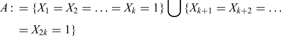
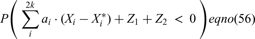
The main result of this paper, Theorem 1, is an explicit lower bound on the relative error for approximating the event

A = {X_{1} = X_{2} = \dots = X_{k} = 1} ⋃ {X_{k + 1} = X_{k + 2} = \dots = X_{2 k} = 1}

(1)

by a one-dimensional functional followed by a Heaviside function, hence by an event:

B : = {a_{1} X_{1} + a_{2} X_{2} + \dots + a_{2 k} X_{2 k} > c},

(2)

where

a_{1}, a_{2}, \dots, a_{2 k}, c

are real numbers. Note that we could always take the event

B

to be

{X_{1} + X_{2} + \dots + X_{k} \geq k},

and then

P (B | A) \approx 0.5

. For a good predictor, we would like

P (B | A)

and

P (A | B)

both close to

1

, not close to

0.5

which translates to the condition:

P (A - B) + P (B - A) \leq ϵ P (A),

for a small constant

ϵ > 0

. (See Condition (7) below, which in terms implies (8) and (11).)

The explicit bound we prove is asymptotically $\frac{1}{16}$ , when $k$ is large enough. In other words, the $ϵ$ in (7) can never go much below $1 / 16$ . This has an extremely important implication for Transformers: compression is not possible without quality loss.

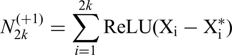
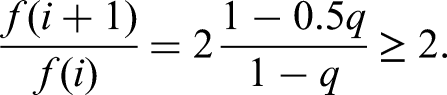
Let us consider the case of $k = 4$ . Let $\vec{X} = (X_{1}, X_{2}, \dots, X_{8}, 1)^{T}$ be a nine-dimensional column vector, with i.i.d Bernoulli variables as entries except the last one, which is always $1$ . We define the event $A$ as in (1). Let

V = (\begin{matrix} 1 & 1 & 1 & 1 & 0 & 0 & 0 & 0 & - 3 \\ 0 & 0 & 0 & 0 & 1 & 1 & 1 & 1 & - 3 \end{matrix})

and let

C = (1, 1)

. Now, consider

C \cdot ReLU (V \cdot \vec{X}),

(3)

where ReLU(.) sets any negative component of a vector to 0 and leaves the positive ones unchanged. Note that the quantity in (3) is greater than or equal to

1

if and only if the event

A

occurs. Meanwhile, an expression of the form

C \cdot ReLU (V \vec{X})

, where

C

and

V

are linear maps of appropriate dimensions, corresponds to the feed-forward layer of a Transformer. Here, the input to the feed-forward layer is the vector

\vec{X}

. In this sense, the event

A

is realized through two fully connected layers encoded in the matrix

V

of a Transformer.

The functional appearing in the definition of event $B$ in (2) can be viewed as corresponding to a single row of the matrix $V$ in the Transformer’s fully connected layer. We choose to use the Heaviside function instead of ReLU to define event $B$ . We could as well use two ReLU activations—which would make the notation more complicated.

Since we have no control of the coefficients $a_{1}, a_{2}, \dots, a_{2 k}$ , the difficulty is to get our bound irrespective of the choice of the coefficients $a_{1}, a_{2}, \dots, a_{2 k}$ . These coefficients could be of different orders of magnitude.

So, summarizing one more time: why is this “approximating $A$ by a one dimensional functional” important at all? The event $A$ represents the logic of two lines in the transformer’s “fully connected” matrix followed by ReLU. On the other hand, the event $B$ would correspond to one line in such a fully connected layer of the transformer. Hence, if it would be possible to approximate $A$ well by $B$ , then one could compress many lines in the transformers into less lines without substantial loss of quality.

The current AI revolution represents a transformation on the scale of the 19th-century Industrial Revolution. This breakthrough is driven almost entirely by Transformers—large language models based on deep neural networks, trained primarily through self-supervised learning.

Transformers contain billions of parameters and require massive datasets—billions of words—for training. At their core, they are deep neural networks with one key innovation: self-attention, introduced in the seminal 2017 paper “Attention Is All You Need,”⁴ which sparked the subsequent wave of advancements in the field.

However, training such models is computationally expensive, often requiring days of supercomputer time. Interestingly, sparse Transformers—models in which only a subset of parameters is active at any given time—can outperform dense ones in terms of quality. Yet, they typically involve more total parameters, making them more costly to train.

Several approaches have been proposed to mitigate this cost,^1–3 such as initializing training with a dense Transformer and transitioning to a sparse model mid-way, thereby reducing computational demands.

Why sparse is higher quality was an open question until our current article. The result of this article shows that one can not compress two lines of the fully connected layer into one without information loss. It is a simple probabilistic result, which, to be understood does not require any knowledge of transformers. But it has deep implications for transformers: since if one could compress lines of the fully connected layer into strictly less lines without information loss, one would then have dense transformers, with equal performance than sparse ones.

It’s worth noting that rigorous theoretical understanding of Transformers remains limited. A few results exist on scaling laws,^5,6 but much of their behavior is still empirically understood.

This article is part of an upcoming series in which we aim to rigorously establish key properties of Transformers from multiple perspectives. Next, we present a numerical example to further illustrate the dense-to-sparse paradigm.

In the next little example we are going to present, the event $A$ contains $l$ disjunctions instead of just $1$ , unlike the situation in our main Theorem 1. This is not to confuse the reader, but this setting of the current example is best for getting an understanding of how multiple layers could be approximated into a single layer and how this would lead to dense Transformers.

Hence, here the example: let $k, l \geq 2$ be two integers. Next, consider more generally than in the rest of the paper, the event $A$ to be defined by:

A : = ⋃_{j = 0}^{l - 1} {X_{k \cdot j + 1} = X_{k \cdot j + 2} = \dots = X_{k \cdot j + k} = 1} .

Let

Y

be the indicator variable for the event

A

, meaning that

Y = 1

A

holds, and

Y = 0

otherwise. Let

V

be the

l

times

l \cdot k

matrix, with the

j

th line consisting of

k

ones in the entries number

j \cdot k + 1

j \cdot k + k

Say $k = 2$ and $l = 3$ . Then, the matrix $V$ would be equal to:

V = (\begin{matrix} 1 & 1 & 0 & 0 & 0 & 0 \\ 0 & 0 & 1 & 1 & 0 & 0 \\ 0 & 0 & 0 & 0 & 1 & 1 \end{matrix}) .

In the current case, the event

A

is given as:

A : = {X_{1} = X_{2} = 1} ⋃ {X_{3} = X_{4} = 1} ⋃ {X_{5} = X_{6} = 1} .

Let

\vec{X} = (X_{1}, X_{2}, \dots, X_{6})^{T}

. Note that for our binary vector

\vec{X}

, the event

A

holds if and only if the vector

V \vec{X}

contains a two somewhere as entry. If we subtract

1

from each entry of that vector, and delete all negative values, then this is equivalent to saying that the sum of the entries (after ReLU with bias

- 1

) must be bigger equal to

1

From what we said previously, we can now express $Y$ by the following formula:

1_{A} = Y = h (C \cdot ReLU (V \vec{X} - \vec{1})),

(4)

where

h (.)

is any function so that

h (x) = 1

for

x \geq 1

and

h (x) = 0

for

x \leq 0

, while

C

is a row vector of length

3

containing only

1

’s. The column vector of length

3

, containing only

1

’s is denoted by

\vec{1}

. Now, if we would add to the matrix

V

a last column of

- 1

’s and to the vector

\vec{X}

a last entry equal to

1

, then we can rewrite the equation (4) to obtain

1_{A} = Y = h (C \cdot ReLU (V \vec{X}))

(5)

As already mentioned in the earlier example, the part

C (ReLU (V \vec{X}))

corresponds to the fully connected layer of a transformer. The original Transformer had

10

such layers placed one after the other. The matrix which in our current toy example is

3

times

6

in the Transformers would be

1000

times

1000

Note that in our current toy example, the matrix $V$ is sparse: it contains many $0$ ’s. On the other hand, it renders the event $A$ perfectly through equation (5). Our matrix $V$ has three rows. We could try to compress it to one row. For this, we would “guess that the event $A$ holds”, when we have:

(1, 1, 1, 1, 1, 1) \cdot \vec{X} = X_{1} + X_{2} + X_{3} + X_{4} + X_{5} + X_{6} \geq 2

(6)

Here the new matrix

V

, would be

V_{n e w} = (1, 1, 1, 1, 1, 1)

and hence contain only one row. So, it would compress three rows into

1

. But it would no longer be sparse. It would still catch the event

A

when it occurs, but it would make errors as soon as, for example,

X_{1} = X_{3} = 1

X_{2} = X_{3} = 1

. In real life, the dense Transformers do exactly the same then what we show in our current example of dimension reduction. We reduce our

3 \times 6

matrix to a smaller matrix with less parameters but, which will make errors in predicting the event

A

. In real life, there can be correlations between the inputs. Imagine, in our current toy-example, that

X_{1}

would strongly correlate with

X_{2}

, and that

X_{3}

would strongly correlate with

X_{4}

, while

X_{5}

would strongly correlate with

X_{6}

. Assume there would be no other strong correlations. Then, our one line (6) could still predict the event

A

with high probability. Why? Because, due to the correlation, the errors might be rare. For example,

X_{1} = X_{3} = 1

, creates an error, because

X_{1}

and

X_{3}

are not part of the same index group. The index groups here would be

{1, 2}

{3, 4}

and

{5, 6}

. For example,

\vec{X} = (1, 0, 1, 0, 0, 0)

would see inequality (6) satisfied, but the event

A

not holding. Hence, a prediction error if we use (6) to predict the event

A

. However, with the correlations as explained, that error might have a small probability because, if

X_{1}

is highly correlated to

X_{2}

but not to

X_{3}

, then

\vec{X} = (1, 0, 1, 0, 0, 0)

, has much less probability than

\vec{X} = (1, 1, 0, 0, 0, 0)

. Hence, the correlations can reduce the probability of prediction error when compressing the transformer, but they do not eliminate these errors completely!

Main part

If the events $A$ and $B$ should be close to each other, that means that the probability $P (A - B) + P (B - A)$ should be small. However, we will have situations where $A$ by itself has polynomial small probability. Then, we need $P (A - B) + P (B - A)$ not just to be small, but small in comparison to $P (A)$ . Hence, the condition we will impose is

P (A - B) + P (B - A) \leq ϵ P (A)

(7)

for a small

ϵ > 0

. This then implies

P (B | A) = \frac{P (A \cap B)}{P (A)} = \frac{P (A) - P (A - B)}{P (A)} \geq 1 - ϵ

(8)

where the very last inequality above was obtained using (7). Using Bayes rule and condition (8), we find

P (A | B) = P (B | A) \cdot \frac{P (A)}{P (B)} \geq (1 - ϵ) \cdot \frac{P (A)}{P (B)} .

(9)

Now, if condition (7) holds, then

\frac{P (A)}{P (B)} \geq \frac{1}{1 + ϵ}

, which applied to (9) implies:

P (A | B) \geq \frac{1 - ϵ}{1 + ϵ} .

(10)

Now we have

0 \geq - 2 ϵ^{2} ⟹ 1 - ϵ \geq 1 - ϵ - 2 ϵ^{2} = (1 + ϵ) \cdot (1 - 2 x)

and hence for every

ϵ > 0

, we have

\frac{1 - ϵ}{1 + ϵ} \geq 1 - 2 ϵ

which when applied to inequality (10), yields

P (A | B) \geq 1 - 2 ϵ .

(11)

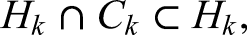
So, we have that for any

ϵ > 0

, Condition (7) implies (8) and (11). The goal of this article is to provide a lower bound beneath which

ϵ > 0

in (7) can not decrease. In other words, we show that the event

B

can not approximate

A

very closely. This means that a depth-2 feed-forward layer cannot be approximated well by a single layer, without incurring a loss in precision. We start with a simplified example, before our Main Theorem (1). In this simplified example, we consider one specific function, the one where all coefficients

a_{i}

are equal to

1

, and show how one cannot approximate

A

well by the event

B

. This example should already give some intuition on what the general case is:

Lemma 1

Let $X_{1}, X_{2}, \dots$ be i.i.d. Bernoulli variables with $P (X_{i} = 1) = p_{k}$ . Consider the event $B^{k}$ defined as:

B^{k} : = {\sum_{i = 1}^{2 k} X_{i} \geq c_{k}}

for some real number

c_{k} > 0

indexed by

k

. Let

A^{k}

be the event:

A^{k} : = {X_{1} = X_{2} = \dots = X_{k} = 1} ⋃ {X_{k + 1} = X_{k + 2} = \dots = X_{2 k} = 1} .

Then, if

P (A^{k} - B^{k}) + P (B^{k} - A^{k}) \leq 0.25 P (A^{k}),

(12)

and if

p_{k} \cdot (1 - p_{k}) \cdot k \to \infty, \,for k \to \infty

(13)

we find that

P (A^{k} | B^{k}) \to 0,

k \to \infty

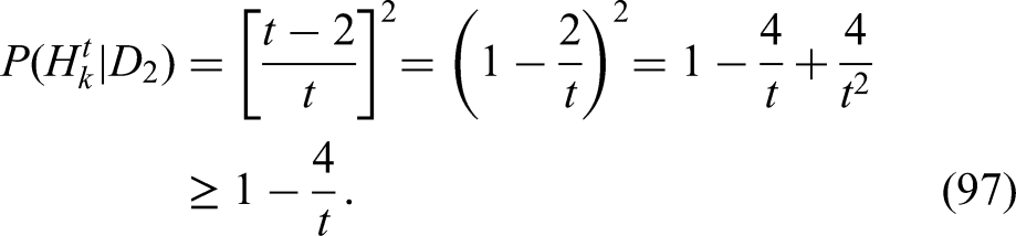
. Hence, one can not approximate the event

A^{k}

well by

B^{k}

. (The condition (13) is there to avoid the trivial case, where you have only a “fixed” small amount of zeros in the string

X_{1} X_{2} \dots X_{2 k}

)

Proof.

Let

E_{1} = {X_{1} = X_{2} = \dots = X_{k} = 1}, E_{2} = {X_{k + 1} = X_{k + 2} = \dots = X_{2 k} = 1},

B_{z}^{k} = {\sum_{i = k + 1}^{2 k} X_{i} \geq 2 k - z} .

The idea is simple: as long as there are more than

O (1)

zeros in the string

X_{1}, X_{2}, \dots, X_{2 k}

, then to have all those zeros present in only one of the two strings

X_{1} \dots X_{k}

X_{k + 1} \dots X_{2 k}

is highly unlikely. This is the same as the second principle of thermodynamics: for a container filled with gas (and no partition), the probability that all particles are only in one half of the space is highly unlikely. Conditional on the event

B^{k}

B_{z}^{k}

, any position of the

0

’s is equally likely. So, we can find an explicit lower bound for having all

0

’s in one string and not in the other given their total number

z

. For this, we place a number of

0

’s equal to

z

in the positions

1, 2, \dots, 2 k

, making sure there are not to

0

’s in the same spot. When you choose at random a place for the first

0

, any position among

1, 2, \dots, 2 k

at first is equally likely. If you want the event

A^{k}

to hold, you need that second

0

to be in same string as the first

0

placed. This is roughly a probability of

0.5

. Assume, without loss of generality the first two

0

’s you placed at random are in the string

X_{1}, X_{2} \dots X_{k}

. Then the third

0

placed at random must also be in the string

X_{1} \dots X_{k}

in order for the event

A^{k}

to hold. This has roughly a probability of

0.5

again. The exact probability is

(k - 2) / 2 k

since two positions are already occupied by the previously place

0

’s. As you keep filling the first string

X_{1} X_{2} \dots X_{k}

with zeros, the probability will decrease. This argument provides the following lower bound:

P (A | B_{z}) \leq {(\frac{1}{2})}^{z} .

(14)

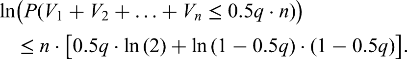
This is a negative exponential small bound in $z$ . As long as we can show that with the event $B$ holding, typically the number of zeros $Z$ defined by:

Z : = 2 k - X_{1} - X_{2} \dots - X_{2 k}

is not too small, we have that

P (A^{k} | B^{k})

is exponentially small rather than close to

1

, which would prove our theorem. Then by law of total probability and using the bound (14), we find for any

z_{0} > 0

that:

P (A^{k} | B^{k}) = P (A^{k} | Z \geq z_{0} \cap B^{k}) \cdot P (Z \geq z_{0} | B^{k}) + P (A^{k} | Z < z_{0} \cap B^{k}) \cdot P (Z < z_{0} | B^{k}) .

(15)

Using the bound (2.8), and assuming

c_{k} < 2 k - z_{0}

, (hence

{Z < z_{0}} \subset B_{k}

, we find:

P (A^{k} | Z \geq z_{0} \cap B_{k}) \cdot P (Z \geq z_{0} | B^{k}) + P (A^{k} | Z < z_{0} \cap B_{k}) \cdot P (Z < z_{0} | B^{k}) \leq {(\frac{1}{2})}^{z_{0}} + P (Z < z_{0} | B^{k})

which together with (2.89) yields:

P (A^{k} | B^{k}) \leq {(\frac{1}{2})}^{z_{0}} + P (Z < z_{0} | B^{k}) .

With the help of the Central Limit Theorem (CLT), we find:

P (A^{k} | B^{k}) = P (A^{k} | Z \geq z_{0}) \cdot P (Z \geq z_{0} | B^{k}) + P (A^{k} | Z < z_{0}) \cdot P (Z < z_{0} | B^{k}) \leq {(\frac{1}{2})}^{z_{0}} + P (Z < z_{0} | B) .

(16)

With the help of the CLT, we find

P (\sum_{i = 1}^{2 k} X_{i} \geq k + p_{k} \cdot k + 2 \sqrt{p_{k} (1 - p_{k}) \cdot k} | E_{1}) < 0.025

for large enough

k

. Same thing holds for

E_{2}

, hence for

A^{k} = E_{1} \cup E_{2}

we find:

P (\sum_{i = 1}^{2 k} X_{i} \geq k + p_{k} \cdot k + 2 \sqrt{p_{k} (1 - p_{k}) \cdot k} | A^{k}) < 0.05.

If the constant

c_{k}

used in the definition of

B^{k}

satisfies:

c_{k} > k + p_{k} \cdot k + 2 \sqrt{p_{k} (1 - p_{k}) \cdot k}

we would have

P (A^{k} \cap B^{k}) \leq 0.05 P (A^{k})

, which contradicts (12).

Hence, we have for large enough $k$ that:

c_{k} \leq k + p_{k} \cdot k + 2 \sqrt{p_{k} (1 - p_{k}) \cdot k} .

(17)

This almost finishes the proof since, when (2.11) holds, we have that

2 k - c_{k} \geq (1 - p_{k}) \cdot k - 2 \sqrt{(1 - p_{k}) \cdot p_{k} \cdot k},

where the right side goes to infinity due to condition (2.7). This implies that under

B^{k}

we have more than

O (1)

0’s, which leads to

P (A^{k} | B^{k})

going to

0

when

k \to \infty

be- cause of our thermodynamical argument. Let us now see this in a slightly more precise way: Take

z_{0}

to be defined:

z_{0} : = \sqrt{0.5 (1 - p_{k}) p_{k} k} .

(18)

Then, using the bound (17), we find:

P (Z \leq z_{0} | B^{k}) \leq \frac{P (Z \leq 0.5 (1 - p_{k}) \cdot k)}{P (Z \leq (1 - p_{k}) \cdot k - 2 \sqrt{k \cdot p_{k})}}

(19)

Now,

Z

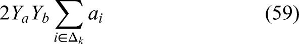
is a binomial with parameters

1 - p_{k}

and

2 k

, so that the expectation is:

E [Z] = 2 (1 - p_{k}) k .

which for large enough k is bigger than

(1 - p_{k})

k - 2 \sqrt{k \cdot p_{k} \cdot (1 - p_{k})}

(thanks to (2.7)). For a binomial variable, when one moves away from the expected value, the probabilities decrease, hence:

\frac{P (Z \leq \sqrt{(1 - p_{k}) \cdot k)}}{P (Z \leq (1 - p_{k}) \cdot k - 2 k \cdot \sqrt{p_{k} \cdot (1 - p_{k})})} \leq \frac{\sqrt{(1 - p_{k}) \cdot k}}{(1 - p_{k}) \cdot k - 2 \sqrt{k \cdot p_{k} \cdot (1 - p_{k})}} \leq \frac{1}{\sqrt{(1 - p_{k}) \cdot k} - 2 \sqrt{p_{k}}}

where the last bound on the right side of the equation above goes to

0

k \to \infty

because of (2.7). Together with (2.13), this implies

P (Z \leq z_{0} | B^{k}) \to 0, \,for k \to \infty .

The last limit above together with (2.10) and the fact that

z_{0}

goes to

\infty

(again due to (2.7)) imply

P (A^{k} | B^{k}) \to 0, f o r k \to \infty

and finishes this proof.

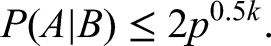
Next, we aim to prove the same result as stated in the lemma above, but for a general linear functional of the form given in (20). In the earlier lemma, we considered the special case where all coefficients satisfy $a_{1} = a_{2} = \dots = a_{2 k} = 1$ . We now remove this restriction and allow arbitrary coefficients $a_{1}, a_{2}, \dots, a_{2 k}$ . This generalization is the content of our main result, Theorem (1), where we show that the event $A$ cannot be closely approximated by the event $B$ defined in (21). The event $B$ is characterized by a linear functional exceeding a given threshold. The quality of this approximation can be measured by the smallest $ϵ > 0$ satisfying condition (7). This minimal $ϵ$ represents the relative approximation error. Theorem 1 establishes a lower bound on $ϵ$ , as stated in (23). Notably, this bound includes a term minus $2 p^{k}$ which corresponds to the probability of the event $A$ . Therefore, the lower bound in (23) is only meaningful when $P (A)$ is sufficiently small—otherwise, the bound could become negative. In the context of our intended Transformer application, this condition is indeed satisfied. With the transformer application we had in mind, the event $A$ represents the occurrence of a specific word at a specific position in the text—an event whose probability is typically quite small.

For example:

Samuel receives a present. He is [Masked]

The most likely guess for the masked word is Happy, so we define the event

A = {[Masked] = ‘ ‘ " {Happy}^{″}} .

In general, the probability of a specific word appearing at a given position in a text is relatively small. Therefore, we can safely assume that

P (A) << 0.5.

(If we consider intermediate layers of a Transformer rather than the final output layer, the prediction pertains not to a word itself but to a feature of the representation at that stage. However, a similar argument still applies.)

Let $q = 2 p (1 - p)$ . The lower bound given in (23) includes negative terms of order $1 / k$ , as well as additional negative contributions captured by the expression in (24). These latter terms tend to zero as $q \cdot k$ increases. Thus, for the bound in (23) to be effective, both $k$ and $q \cdot k$ must grow. If $q$ or $k$ remain small our bound does not work. This implies that the number of zeros in the binary string $X_{1}, X_{2}, \dots, X_{2 k}$ must also grow. However, this growth can be quite slow and still suffice for our result to hold. For instance, if the expected number of zeros is only $\ln (k)$ , while the rest of the string consists of ones, the bound still yields meaningful results.

In other words, our bound applies across a wide range of scenarios. We may even allow the probability $p = P (X_{i} = 1)$ to vary with $k$ writing $p = p_{k}$ . In particular, it ensures that $ϵ$ cannot remain below $1 / 16$ by more than an infinitesimal amount, while $k$ and $q k$ grow to infinity.

Empirically, this phenomenon already appears for fairly moderate values of $k$ . (See the “Simulations” section.)

Theorem 1

Assume $p \in (0, 1)$ and let $q = 2 p (1 - p)$ . Let $a_{1}, a_{2}, \dots, a_{2 k}, c$ be any real numbers and let

S_{k} : = a_{1} X_{1} + a_{2} X_{2} + \dots + a_{2 k} X_{2 k} .

(20)

Let

A

be the event:

A : = {X_{1} = X_{2} = \dots = X_{k} = 1} ⋃ {X_{k + 1} = X_{k + 2} = \dots = X_{2 k} = 1}

and let

B

be the event defined:

B : = {S_{k} \geq c} .

(21)

Let $ϵ > 0$ . Then, inequality

P (A - B) + P (B - A) \leq ϵ P (A),

(22)

implies

ϵ \geq 0.25 \cdot (1 + \frac{1}{k})^{- 1} [0.25 (1 - 2 (E (q k))) - 2 p^{k} - \frac{2}{k}],

(23)

where

E (q k)

is defined by:

E (k q) = \exp (- 0.05 q k) + 2 \cdot \frac{\exp (\frac{1}{24})}{(q k)^{0.25} \sqrt{0.5 π}} + {0.75}^{(q k)^{0.25}} + {0.99}^{{q k}^{0.25}} + \frac{10}{(q k)^{0.25}} .

(24)

(Note that inequality (22) when

ϵ > 0

is small, shows that

B

approximates

A

closely. We could view

ϵ > 0

as the size of the relative error of approximating

A

B

. Hence, inequality (23) yields a lower bound on the approximation error as

k

grows and assuming that

q \cdot k

also goes to infinity at the same time. This means that we can not approximate the event

A

very closely by using only one functional followed by Heaviside function).

Proof.

Let $E_{1}$ be the event

E_{1} : = {X_{1} = X_{2} = \dots = X_{k} = 1}

and let

E_{2}

be the event

E_{2} : = {X_{k + 1} = X_{k + 2} = \dots = X_{2 k} = 1} .

Let

D_{1}

be the event that among the first

k

bits, there are exactly

k - 1

equal to

1

, hence

D_{1} = {X_{1} + X_{2} + \dots + X_{k} = k - 1}

similarly, we define the event

D_{2}

D_{2} : = {X_{k + 1} + X_{k + 2} + \dots + X_{2 k} = k - 1} .

So, similarly to our previous notation, we put:

A : = E_{1} \cup E_{2}

and

B = {a_{1} X_{1} + a_{2} X_{2} + \dots + a_{2 k} X_{2 k} \geq c} = {S_{k} \geq c} .

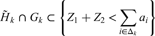
Now, we want to show that Condition (7) can not hold for

ϵ > 0

small. We do the proof by contradiction. So, let us assume on the contrary that (7) holds for

ϵ > 0

close to

0

. We have shown, that (7) implies (8). But, (8) means that:

P (S_{k} \geq c | E_{1} \cup E_{2}) \geq 1 - ϵ

(25)

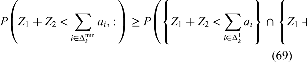
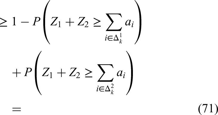
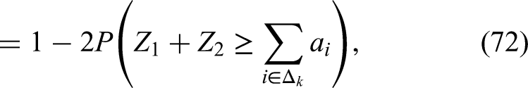
So, let us first outline the main idea of the proof: clearly (25) implies that when

E_{1}

holds, then

S_{k} \geq c

also holds with high probability and the same is true when

E_{2}

holds. Now, conditional on

E_{1}

, we have that

S_{k}

is equal to:

a_{1} + \dots + a_{k} + a_{k + 1} X_{k + 1} + \dots + a_{2 k} X_{2 k} .

(26)

Hence,

P (S_{k} \geq c | E_{1}) = P (a_{1} + a_{2} + \dots + a_{k} + a_{k + 1} X_{k + 1} + a_{k + 2} X_{k + 2} + \dots + a_{2 k} X_{2 k} \geq c) \geq 1 - ϵ

(27)

But, when we go over to conditioning on

D_{1}

instead of

E_{1}

, then the event

A

is likely to no longer hold. This would imply that

P (S_{k} \leq c | D_{1})

should hold with high probability. (Hence

S_{k}

suddenly becomes likely smaller than

c

instead of larger.) But going from conditioning on

E_{1}

to conditioning on

D_{1}

, all we did is turn one bit from the first

k

into

0

. Hence, we subtract a random quantity

Z_{1}

from the variable (26), where

Z_{1}

is defined by

P (Z_{1} = a_{j}) = \frac{1}{k}, \forall j \in {1, 2, \dots, k} .

So,

P (S_{k} \leq c | D_{1}) = P (a_{1} + a_{2} + \dots + a_{k} + a_{k + 1} X_{k + 1} + a_{k + 2} X_{k + 2} + \dots + a_{2 k} X_{2 k} - Z_{1} \leq c)

(28)

Let us calculate the expectation:

E [Z_{1}] = \frac{1}{k} \sum_{i = 1}^{k} a_{i} .

(29)

and the standard deviation of the variable (26) is:

σ : = \sqrt{V A R [a_{k + 1} X_{k + 1} + \dots + a_{2 k} X_{2 k}]} = \sqrt{p \cdot (1 - p)} \sqrt{\sum_{i = k + 1}^{2 k} a_{i}^{2}} .

(30)

Now, assume that the CLT applies to the variable (26). (For our proof below, we do not make this assumption. This assumption of CLT holding is only used for our heuristic argument, and we believe it might more or less hold in many cases with real-life data). Then, we get that the variable (26) is approximately a normal with expectation

μ = a_{1} + a_{2} + \dots + a_{k} + p (a_{k + 1} + a_{k + 2} + \dots + a_{2 k})

and standard deviation

σ

, given in (30). That would be to say that “approximately “ (27) can be rewritten as:

P (N (μ, σ^{2}) \geq c) \geq 1 - ϵ .

(31)

But, conditioning on

D_{1}

, we obtain that

N (μ, σ^{2}) - Z_{1} < c

(32)

must hold with high probability according to (28) This reversal of likely inequality going from (31) to (32) is not possible if

Z_{1}

is typically a much smaller order than

σ

! Now, typically (30) is much larger than (29), except in situations where, for example, all the first

k

coefficients

a_{1}, a_{2}, \dots, a_{k}

are large and the subsequent

k

coefficients

a_{k + 1}, a_{k + 2}, \dots, a_{2 k}

are close to

0

. But in that case, we could do the same argument using

E_{2}

and

D_{2}

instead of

E_{1}

and

D_{1}

. Let us be more precise. By Jensen’s inequality we have

\frac{1}{k} \sum_{i = 1}^{k} a_{i} \leq \sqrt{\sum_{i = 1}^{k} \frac{a_{i}^{2}}{k}} = \frac{1}{\sqrt{k}} \cdot \sqrt{\sum_{i = 1}^{k} a_{i}^{2}}

(33)

Hence, the expression

\sqrt{\sum_{i = 1}^{k} a_{i}^{2}}

is an order

O (\sqrt{k})

larger than the left most side of (33). The two expressions (29) and (30) above are defined each for different sets of indexes. One is for

i = 1, 2, \dots, k

and the other for

i = k, k + 1, k + 2, \dots, 2 k

. So, a priori (33) does not directly apply. However, when instead of

\sqrt{\sum_{i = 1}^{k} a_{i}^{2}}

, we take the maximum

max {\sqrt{\sum_{i = 1}^{k} a_{i}^{2}}, \sqrt{\sum_{i = k + 1}^{2 k} a_{i}^{2}}}

then, (33) with that replacement holds. Let us now show the formal proof. One of the difficulties will be that we can not assume normal approximation for the variable (26) since the coefficients

a_{i}

for

i = 1, 2, \dots, 2 k

may all be of different orders and we don’t want to impose any restriction there. So, again, we assume Condition (7) to hold, which is to say that

P (S_{k} \geq c | E_{1} \cup E_{2}) \geq 1 - ϵ

Starting from last inequality above, we find:

1 - ϵ \leq

(34)

\leq P (S_{k} \geq c | E_{1} \cup E_{2}) =

(35)

= \frac{P ({S_{k} \geq c} \cap (E_{1} \cup E_{2}))}{P (E_{1} \cup E_{2})} =

(36)

= \frac{P (({S_{k} \geq c} \cap E_{1}) ⋃ ({S_{k} \geq c} \cap E_{2}))}{P (E_{1} \cup E_{2})} \leq

(37)

\leq \frac{P ({S_{k} \geq c} \cap E_{1}) + P ({S_{k} \geq c} \cap E_{2})}{P (E_{1} \cup E_{2})} =

(38)

= P (S_{k} \geq c | E_{1}) \cdot \frac{P (E_{1})}{P (E_{1} \cup E_{2})} + P (S_{k} \geq c | E_{2}) \cdot \frac{P (E_{2})}{P (E_{1} \cup E_{2})} \leq

(39)

\leq P (S_{k} \geq c | E_{1}) \cdot \frac{P (E_{1})}{P (E_{1} \cup E_{2})} + \frac{P (E_{2})}{P (E_{1} \cup E_{2})} .

(40)

Now, if $p = P (X_{i} = 1)$ , then we find

\frac{P (E_{1})}{P (E_{1} \cup E_{2})} = \frac{P (E_{2})}{P (E_{1} \cup E_{2})} = \frac{p^{k}}{2 \cdot p^{k} - p^{2 k}} = \frac{1}{2 - p^{k}} .

Applying this to (34), we find:

P (S_{k} \geq c | E_{1}) \geq 1 - p^{k} - 2 ϵ

(41)

Conditional on

E_{1}

, we have that

S_{k}

is equal to the variable (26), so that (41) implies

P (a_{1} + \dots + a_{k} + a_{k + 1} X_{k + 1} + \dots + a_{2 k} X_{2 k} \geq c) \geq 1 - p^{k} - 2 ϵ

(42)

Now, recall that

D_{1}

is the event

D_{1} : = {X_{1} + X_{2} + \dots + X_{k} = k - 1}

Hence, when

D_{1} \cap E_{2}^{c}

holds, then

A = E_{1} \cup E_{2}

does not hold. Hence

D_{1} \cap E_{2}^{c} \cap {S_{k} \geq c} \subset B - A .

(43)

where again

B = {S_{k} \geq c}

. By Condition (7), we have

P (B - A) \leq ϵ P (A)

and hence with the help of (43), we find:

P (D_{1} \cap E_{2}^{c} \cap {S_{k} \geq c}) \leq ϵ P (E_{1} \cup E_{2})

and hence

P (D_{1} \cap {S_{k} \geq c}) \leq ϵ P (E_{1} \cup E_{2}) + P (E_{2}) .

Dividing the last inequality above by

P (D_{1})

, we find:

P (S_{k} \geq c | D_{1}) \leq ϵ \frac{P (E_{1}) + P (E_{2})}{P (D_{1})} + \frac{P (E_{2})}{P (D_{1})} = \frac{2 ϵ}{k} + \frac{1}{k} .

(44)

Here, for the very last equation above, we used that

P (D_{1})

k

-times larger than

P (E_{1})

and

P (E_{2})

each. Now, Conditional on

D_{1}

, the variable

S_{k}

is equal to the variable (26) minus

Z_{1}

, where

Z_{1}

is the random variable which can take any of the values

a_{1}, a_{2}, \dots, a_{k}

with equal probability

1 / k

. Hence, we obtain from (44), that

\begin{aligned} P (S_{k} \geq c | D_{1}) = \\ = P (a_{1} + \dots + a_{k} + a_{k + 1} X_{k + 1} * + \dots \\ + a_{2 k} X_{2 k} * - Z_{1} \geq c) \leq \frac{2 ϵ}{k} + \frac{1}{k} \end{aligned}

Where we take

X_{1} *, X_{2} *, \dots, X_{2 k} *

to be i.i.d. binary random variable independent of the sequence

X_{1}, X_{2}, \dots, X_{2 k}

, but having same probability distribution. Now, we multiply the inequality inside the probability above by

- 1

and obtain

P (- a_{1} - \dots - a_{k} - a_{k + 1} X_{k + 1} * - \dots - a_{2 k} X_{2 k} * + Z_{1} \leq - c) \leq \frac{2 ϵ}{k} + \frac{1}{k},

so that

P (- a_{1} - \dots - a_{k} - a_{k + 1} X_{k + 1} * - \dots - a_{2 k} X_{2 k} * + Z_{1} \geq - c) \geq 1 - \frac{2 ϵ}{k} - \frac{1}{k} .

The last inequality above, together with (42) imply

P (a_{k + 1} (X_{k + 1} - X *_{k + 1}) + \dots + a_{2 k} (X_{2 k} - X *_{2 k}) + Z_{1} \geq 0) \geq 1 - p^{k} - 2 ϵ \cdot (1 + \frac{1}{k}) - \frac{1}{k} .

(45)

Now let

Z_{2}

be a random variable which takes on values from the set

{a_{k}, a_{k + 1}, \dots, a_{2 k}}

with equal probability

1 / k

. Then, a similar argument but using

E_{2}

and

D_{2}

instead of

E_{1}

and

D_{1}

leads to an equation similar to equation (45), given as follows:

P (a_{1} (X_{1} - X *_{1}) + \dots + a_{k} (X_{k} - X *_{k}) + Z_{2} \geq 0) \geq 1 - p^{k} - 2 ϵ \cdot (1 + \frac{1}{k}) - \frac{1}{k}

(46)

Together, (45) and (46) imply:

P (\sum_{i}^{2 k} a_{i} \cdot (X_{i} - X_{i} *) + Z_{1} + Z_{2} \geq 0) \geq 1 - 2 p^{k} - 4 ϵ \cdot (1 + \frac{1}{k}) - \frac{2}{k} .

(47)

Now the variable

\sum_{i}^{2 k} a_{i} \cdot (X_{i} - X_{i} *)

has expectation

0

and standard deviation

\sqrt{VAR [\sum_{i = 1}^{2 k} a_{i} \cdot (X_{i} - X_{i} *)]} = \sqrt{2 p (1 - p) \sum_{i = 1}^{2 k} a_{i}^{2}}

(48)

which typically is much bigger than

Z_{1} + Z_{2}

, hence making the inequality (47) very unlikely to hold. Indeed, if that variable has much bigger standard deviation than the typical order of magnitude of

Z_{1} + Z_{2}

, and since that variable is symmetric around the origin, than we would expect that the probability of (47) to be about

0.5

and not close to

1

! (Again, we look at the case where

k

is large and hence

2 p^{k}

is small. So, then if additionally

ϵ > 0

would be small, then the expression on the right side of (47) would be close to

1

. That contradiction is what our proof that

ϵ > 0

can not be too small is based on.) Now, to prove this formally, there is still some work, since a random variable could theoretically have most of its mass close to

0

, and only a very small mass very far away, creating a large standard deviation…. We can not assume CLT to apply to the sum inside the probability on left side or (47). Otherwise, we would be done with our proof for lower bound for

ϵ > 0

. Indeed, if the CLT would hold, then the probability on the left side of (47) would be about

0.5

, which would then turn (47) into a lower bound for

ϵ

. Sadly enough, however, since the coefficients

a_{i}

might be of many different orders, we can not assume the CLT to hold! Now, we have to consider the possibility that among the coefficients

a_{i}

, there should be many

0

’s.

First case: there are more than $75 %$ of the coefficients $a_{1}, a_{2}, \dots, a_{2 k}$ equal to 0.

Let $J_{k} \subset [0, 2 k]$ be the integer subset for which the coefficients $a_{i}$ are $0$ :

J_{k} = {j \in [1, 2 k] | a_{j} = 0}

Let

A_{J}

be the event that either all

X_{i}

’s with

i \in J_{k} \cap [1, k]

are

1

or all coefficient with index

i

contained in

i \in J_{k} \cap (k, 2 k]

. Hence,

A_{J} = (⋂_{i \in J_{k} \cap [1, k]} {X_{i} = 1}) ⋃ (⋂_{i \in J_{k} \cap (k, 2 k]} {X_{i} = 1})

For

A

to hold, we have that

A_{J}

needs to be satisfied, and hence

A \subset A_{J} .

leading to

P (A | B) \leq P (A_{j} | B)

(49)

But, since

A_{j}

is only involved with the

X_{i}

’s for which

a_{i} = 0

, we have that

A_{j}

is independent of

B

, and hence:

P (A_{j} | B) = P (A_{J})

(50)

We assume here that there are at least

75 %

of coefficients

a_{i}

with

i \in [0, 2 k]

, for which

a_{i} = 0

. That means in each integer interval

[1, k]

and

(k, 2 k]

there are at least

0.5 k

indices

i

for which

a_{i} = 0

. Again,

p

is the probability to have a one:

P (X_{i} = 1) = p

. Due to independence, the event that for all

j

[1, k]

, with

a_{j} = 0

, we have

X_{i} = 1

, has a probability less than

p^{0.5 k}

. The same is true for the event to have

X_{i} = 1

for all

i \in J \cap (k, 2 k]

for which

a_{j} = 0

. Hence,

P (A_{j}) \leq 2 p^{0.5 k},

which together with (49) and (50) implies

P (A | B) \leq 2 p^{0.5 k} .

Using the very last inequality above together with (11) implies

ϵ \geq 0.5 - p^{0.5 k} .

We are now ready to look at second case:

Second case: here we assume that at least $25 %$ of the coefficients $a_{1}, a_{2}, \dots, a_{2 k}$ are non-zero. To start with, let us define:

N_{2 k}^{(+ 1)}

to be the number of indexes in

[1, 2 k]

for which

X_{i} - X_{i} * = + 1

. Hence

N_{2 k}^{(+ 1)} = \sum_{i = 1}^{2 k} ReLU (X_{i} - X *_{i})

and let

N_{2 k}^{(- 1)} = \sum_{i = 1}^{2 k} ReLU (- X_{i} + X *_{i})

Note that both

N_{2 k}^{(+ 1)}

and

N_{2 k}^{(- 1)}

are Binomial variables with parameters

2 k

and

p \cdot (1 - p)

. Let

N_{2 k}^{(\neq 0)} = N_{2 k}^{(+ 1)} + N_{2 k}^{(- 1)}

. Again, this is a Binomial variable with parameters

2 k

and

2 p (1 - p)

So, we are going to “simulate” for which coefficients $i$ in $[1, 2 k]$ , we have $X_{i} - X_{i} * = + 1$ and for which we have $X_{i} - X_{i} * = - 1$ . This representation will be very useful for our proof. Let us first give an example:

Let $k = 7$ . Let us define the random variables $W_{i}$ as follows: $W_{i} = X_{i} - X_{i}^{*}$ . The variable $W_{i}$ are i.i.d. and

P (W_{i} = 1) = P (W_{i} = - 1) = p (1 - p), P (W_{i} = 0) = p^{2} + (1 - p)^{2} .

We consider the string

W_{1} W_{2} \dots W_{2 k}

. We are first going to flip a coin to determine which of the

W_{i}

’s are such that

| W_{i} | = 1

. When

| W_{i} | = 1

, this means that either

W_{i} = + 1

W_{i} = - 1

. In that case, we write

W_{i} \in U

, where

U

is the set

U = {- 1, 1}

. The coin is not fair, but has a side with a

U

written on it and the other side with

0

. (Because, when

X_{i}

is not in

U

then it is equal to

0

. So, after a simulation, here is what we obtained:

\vec{W} : = (W_{1} W_{2} \dots W_{2 k}) = (00 U U U U 0 U U 0 U U 00) .

(51)

At this stage of the “simulation” of

\vec{W}

, we have already determined which

W_{i}

’s are equal to

0

. But among those which are not

0

, we have not yet determined which among the

U

’s in the above string correspond to

+ 1

and which ones correspond to

- 1

. Note that according to our notation, the total number of

U

’s is equal to

N_{2 k}^{(+ 1)} + N_{2 k}^{(- 1)}

, in the present simulation given in (51), we find

N_{2 k}^{(+ 1)} + N_{2 k}^{(- 1)} = 8

. Next, we are going to determine which of the

W_{i}

’s satisfying

W_{i} \in U

are such that

W_{i} = + 1

and for which of those we have

W_{i} = - 1

. It is easy to see that given (51), the

W_{i}

’s for which

W_{i} \in U

, have equal probability to be

+ 1

- 1

independently of each other. This is to say, that conditional on the total number of

U

’s in

\vec{W}

being equal to

r

, the number of

+ 1

’s is binomial:

L (N_{2 k}^{+ 1} | N_{2 k}^{+ 1} + N_{2 k}^{- 1} = r) = B i n o m i a l (r, 0.5) .

In other words, we can flip a fair coin to determine which of the

W_{i} \in U

are

+ 1

and which are

- 1

. For large

r

, we will have about

0.5 r

which are

+ 1

and

0.5 r

which are

- 1

, this assuming:

N_{2 k}^{+ 1} + N_{2 k}^{- 1} = r .

(52)

Instead of flipping a fair coin independently to determine the

+ 1

and the

- 1

’s for every index

i

, we will pick two sets

I_{1}

and

I_{2}

of same size among the indices

i

for which

W_{i} \in U

. In the case of our current numeric example, (51), the set of indices with

W_{i} \in U

are

I : = {3, 4, 5, 6, 8, 9, 11, 12}

. We pick in that set with equal probability among all subsets of size

4

, a subset

I_{1}

: We obtained:

I_{1} = {3, 4, 8, 9} .

Then,

I_{2} = I - I_{1} = {5, 6, 11, 12} .

Now, we flip a coin to determine which of the subsets

I_{1}

I_{2}

will host the

+ 1

’s and which will have the

- 1

’s. (That is, we have a variable

Y_{a}

so that if

Y_{a} = 1

, then

I_{1}

gets the

+ 1

’s and if

Y_{a} = 0

we fill

I_{1}

with

- 1

’s. ) In our simulation, we obtained

Y_{a} = 1

, so that we put

+ 1

for the

W_{i}

s with indices in

I_{1}

and

- 1

for indices in

I_{2}

. This would lead to a simulated

\vec{W}

\vec{W} = (0, 0, 1, 1, - 1, - 1, 0, 1, 1, 0, - 1, - 1, 0, 0) .

(53)

The above binary vector is only an intermediate “simulation” and not yet the final

\vec{W}

. To get the final

\vec{W}

we are going to modify the above one given in (53). The reason is that In (53), we have that same number of

+ 1

as we have

- 1

’s, so that

N_{2 k}^{(+ 1)} - N_{2 k}^{(- 1)} = 0

. In general, that difference has a small probability to be

0

, so the simulation so far given in (53) does not yet have the same probability distribution as the true

\vec{W}

. What we will do to get the exact distribution is to simulate the difference

| N_{2 k}^{(+ 1)} - N_{2 k}^{(- 1)} |

given the already simulated

N_{2 k}^{(+ 1)} + N_{2 k}^{(- 1)} = r

. That means we simulate the difference in size between the sets

I_{1}

and

I_{2}

. Note that, conditional on (52), we have

N^{(+ 1)})_{2 k}

is a binomial variable with parameters

r

and

0.5

. Note that when condition (52) holds, then

N {2 k}^{(- 1)} = r

and hence

N_{2 k}^{(+ 1)} - N_{2 k}^{(- 1)} = 2 N_{2 k}^{(+ 1)} - r

. The absolute value of the difference in size of the sets

I_{1}

and

I_{2}

can be written as:

| N_{2 k}^{(+ 1)} - N_{2 k}^{(- 1)} | = | 2 N_{2 k}^{(+ 1)} - r |

(54)

and hence we can simulate the left side of (54) conditional on (52), by simulating a Binomial variable

B

with parameters

r

and

0.5

and then taking for the simulated value of (54), the value:

| 2 B - r |

. So, in our numeric example (51), we had

r = 8

. We simulated (54) given condition (52) and obtained that the difference in size between the sets

I_{1}

and

I_{2}

should be

4

. This means that we need to remove two elements from one of the sets

I_{1}

I_{2}

and add it to the other set in order to obtain a difference in size of

4

. We flip first a coin to determine in which of the two sets

I_{1}

I_{2}

we remove the set of two points, and which of these sets the two points get added to. The set of size

2

in our example, will be denoted by

Δ_{k}

. The coin is represented by a Bernoulli variable

Y_{b}

, which is independent of anything else, and so that

P (Y_{b} = 1) = P (Y_{b} = 0) = 0.5

. When

Y_{b} = 1

, we remove two elements from

I_{1}

(meaning

Δ_{k} \subset I_{1}

) and otherwise from

I_{2}

. Assume we flip the coin and get

Y_{b} = 1

. Then that means that we pick

Δ_{k}

to be a subset of

I_{1}

. We pick among all subsets of size two from

I_{1}

. In our current numeric simulation, we would found

Δ_{k} = {8, 9}

. Hence, from (53), we are going to change the sign of

W_{8}

and

W_{9}

leading to

\vec{W} = (0, 0, 1, 1, - 1, - 1, 0, - 1, - 1, 0, - 1, - 1, 0, 0) .

(55)

After this final step, we get in (55) a binary string with the desired distribution of

\vec{W}

. If you compare (53) with the final result (55), we see that the only change happened by changing the sign of the

W_{i}

’s with index

i

Δ_{k}

. This version of

\vec{W}

given in (55), is our final version representing the simulation of

\vec{W}

Why do we need this representation of our data using the sets $I_{1}$ , $I_{2}$ and $Δ_{k}$ ? The answer is as follows: we want to lower bound $ϵ > 0$ to show that we can not approximate the event $A$ very closely by $B$ , (check definition of $A$ and $B$ and $ϵ$ in the statement of this current Theorem.) Now, such a lower bound is based on inequality (47) and noticing that when $k$ is not very small, typically the standard deviation given in (48)i is a bigger order than $Z_{1} + Z_{2}$ . Recall that $Z_{1}$ and $Z_{2}$ are two of the numbers $a_{1}, a_{2}, \dots, a_{2 k}$ chosen at random. So, if the CLT would apply for the sum inside the probability in (47), then the probability on the left of (47) would be about $0.5$ . (Again assuming that $Z_{1} + Z_{2}$ is of smaller order than the standard deviation (48). Hence, you would get a bound close to $0.5$ for the probability in (47), which then translates into a lower bound for $ϵ$ . Now the problem is that we can not be sure that the CLT applies. First, because for CLT you can not have a few terms among $a_{1}, a_{2}, \dots, a_{2 k}$ which are larger than the sum of all the others. But there is no guarantee for that. Second, we want a bound which is true for all sequences $(a_{1}, a_{2}, \dots, a_{k})$ and not just one specific, which means we could not use the regular CLT, but would need a uniform one. So instead of CLT, we use our simulation-representation” of $\vec{W}$ . Meaning, it is going to be the fluctuation of $Δ_{k}$ , which will be used instead of CLT. So, in other words, in order to lower bound $ϵ$ we need a lower bound on the following probability:

P (\sum_{i}^{2 k} a_{i} \cdot (X_{i} - X_{i} *) + Z_{1} + Z_{2} < 0)

(56)

So instead of taking right away the sum:

\sum_{i}^{2 k} a_{i} \cdot (X_{i} - X_{i} *) = \sum_{i = 1}^{2 k} a_{i} W_{i}

(57)

we are first going to take our simulation (53), which is not yet the final version. With this stage of simulation replacing the final

\vec{W}

in the right side of 112 by (53), we get the expression:

Y_{a} (\sum_{i \in I_{1}} a_{i} - \sum_{i \in I_{2}} a_{i})

(58)

when we then go over to using the “final version” of

\vec{W}

as given in 55. We have to subtract the term:

2 Y_{a} Y_{b} \sum_{i \in Δ_{k}} a_{i}

(59)

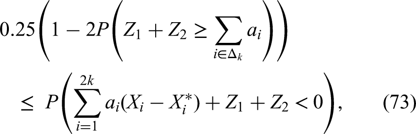
This then leads to formula (61) below. Now, by symmetry expression (58), has a probability to be less or equal to

0

of at least

0.5

. Same thing for expression59. But when both these expressions are strictly negative, we only need (59) to be strictly larger in absolute value than

Z_{1} + Z_{2}

for the inequality inside the probability (56) to hold. In other words, the probability (56) shouldn’t be much less than

0.25

following this argument. And this in terms, allows to get the lower bound (77) on

ϵ

. Of course, we also need to show that with high probability

Z_{1} + Z_{2}

is strictly less than

\sum_{i \in Δ_{k}} a_{i}

. For this, we assume without loss of generality that all coefficients

a_{i}

are non-negative. Now,

Δ_{k}

has typically a size of order

O (\sqrt{k})

. so, when you pick at random

\sqrt{k}

terms from a set of positive numbers to build a some, than that is usually bigger than when you pick only two at random! (Provided

k >> 2

.) For the proof, see Lemma (5) below.

Let us give the precise definition of our “simulation” representation of $\vec{W}$ , hence of $Y_{a}, Y_{b}, I_{1}, I_{2}, Δ_{k}$ :

Simulate a Binomial variable with parameters $2 k$ and $2 p (1 - p)$ to get $N_{2 k}^{(\neq 0)}$ . (That is the number of indexes $i \in [1, 2 k]$ for which $X_{i} - X *_{i} \neq 0$ ) Say you obtain the number $2 r$ . (We assume the number to be even to simplify notations).

Choose a random set $I$ of the integer interval $[1, 2 k]$ with size with size $2 r$ . This will be the set of indexes $i$ for which $X_{i} - X_{i} * \neq 0$ .

Select with equal probability a subset $I_{1}$ of $I$ of size $r$ among all subsets of that size. Let $I_{2}$ be the complement in $I$ : $I_{2} : = I - I_{1}$ . One of the subsets will roughly correspond to the indexes with $X_{i} - X_{i} * = + 1$ , and the other will correspond to the indexes with $X_{i} - X_{i} * = - 1$ . Why do we say roughly? Because both sets $I_{1}$ and $I_{2}$ have equal size at this stage of the simulation and at next stage we will correct that to not make them exactly equal.

Next, we flip a fair coin $Y_{a}$ to decide which of the two set $I_{1}$ or $I_{2}$ will have the $+ 1$ ’s and which will have the $- 1$ ’s. Hence, for which we will have $X_{i} - X_{i} * = + 1$ and which will correspond to $X_{i} - X_{i} * = - 1$ . So:

P (Y_{a} = 1) = P (Y_{a} = - 1) = 0.5

and hence we can already approximate the sum:

\sum_{i = 1}^{2 k} a_{i} (X_{i} - X_{i} *) \approx Y_{a} \cdot (\sum_{i \in I_{1}} a_{i} - \sum_{i \in I_{2}} a_{i}) .

(60)

This is only an approximation because the sets

I_{1}

and

I_{2}

in our simulation have exactly the same size and this is going to be corrected later on.

Since $I_{1}$ and $I_{2}$ have exactly the same size, we need to correct the approximation formula (60) for that. So, we are going to choose a random set $Δ_{k}$ in $I_{1}$ or in $I_{2}$ in the next for which we will change the sign on that set. This will be done in the next bullet point. But here we first need to decide if we want to reduce $I_{1}$ or $I_{2}$ . For this, we flip a fair coin $Y_{b}$ , so that

P (Y_{b} = 1) = P (Y_{b} = - 1) = 0.5

Y_{b} = 1

, then

Δ_{k} \subset I_{1}

, while if

Y_{b} = - 1

, then

Δ_{k} \subset I_{2}

At this stage, we simulate the size of the subset $Δ_{k}$ with distribution $| N_{2 k}^{(+ 1)} - N_{2 k}^{(- 1)} |$ given the sum be $r$ . Hence, we draw from the conditional Law:

L (| N_{2 k}^{(+ 1)} - N_{2 k}^{(- 1)}) | | N_{2 k}^{(+ 1)} + N_{2 k}^{(- 1)} = 2 r)

to obtain the number

δ \geq 0

We now choose the random set $Δ_{k}$ : if $Y_{b} = 1$ , then we choose with equal probability from all subsets of $I_{1}$ with size $δ$ . If, on the contrary, $Y_{b} = - 1$ , then we choose from all subsets of $I_{2}$ of size $δ$ . This then defines the simulated random set $Δ_{k}$ . We can now correct the approximation formula (60), into an exact formula:

\sum_{i = 1}^{2 k} a_{i} (X_{i} - X_{i} *) = Y_{a} \cdot (\sum_{i \in I_{1}} a_{i} - \sum_{i \in I_{2}} a_{i}) - 2 Y_{a} Y_{b} \sum_{i \in Δ_{k}} a_{i}

(61)

We are now ready to show the detail of what we already outlined, that is, the obtaining of our lower bound (77) for

ϵ > 0

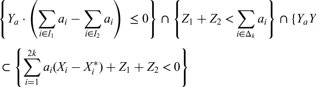
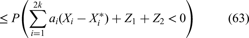
We can assume that $a_{1}, a_{2}, \dots, a_{2 n} \geq 0$ without lack of generality. So, that is what we do from here on. Note that when in the expression on the right of (61), the first sum is less or equal to $0$ and the sum $\sum_{i \in Δ_{k}} a_{i}$ strictly exceeds $Z_{1} + Z_{2}$ , while $Y_{a} Y_{b} = 1$ , then the expression on the left of (61) plus $Z_{1} + Z_{2}$ is strictly below $0$ :

\begin{aligned} {Y_{a} \cdot (\sum_{i \in I_{1}} a_{i} - \sum_{i \in I_{2}} a_{i}) \leq 0} \cap {Z_{1} + Z_{2} < \sum_{i \in Δ_{k}} a_{i}} \cap {Y_{a} Y_{b} = 1} \subset \\ \subset {\sum_{i = 1}^{2 k} a_{i} (X_{i} - X_{i} *) + Z_{1} + Z_{2} < 0} \end{aligned}

which implies

P ({Y_{a} \cdot (\sum_{i \in I_{1}} a_{i} - \sum_{i \in I_{2}} a_{i}) \leq 0} \cap {Z_{1} + Z_{2} < \sum_{i \in Δ_{k}} a_{i}} \cap {Y_{a} Y_{b} = 1}) \leq

(62)

\leq P (\sum_{i = 1}^{2 k} a_{i} (X_{i} - X_{i} *) + Z_{1} + Z_{2} < 0)

(63)

Note that

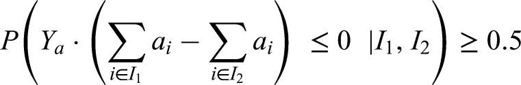
I_{1}, I_{2}, Y_{a}, Y_{b}

are independent of each other. So, when conditioning on

I_{1} a n d I_{2}

, we find:

P (Y_{a} \cdot (\sum_{i \in I_{1}} a_{i} - \sum_{i \in I_{2}} a_{i}) \leq 0 | I_{1}, I_{2}) \geq 0.5

Note that

Y_{a} Y_{b} = 1

, simply means that

Y_{b} = Y_{a}

. So, once

Y_{a}

is determined, the probability that

Y_{b}

be equal to

Y_{a}

0.5

, and hence:

P ({Y_{a} \cdot (\sum_{i \in I_{1}} a_{i} - \sum_{i \in I_{2}} a_{i}) \leq 0} \cap {Z_{1} + Z_{2} < \sum_{i \in Δ_{k}} a_{i}} \cap {Y_{a} Y_{b} = 1} | I_{1}, I_{2}) =

(64)

= 0.5 \cdot 0.5 \cdot P (Z_{1} + Z_{2} < \sum_{i \in Δ_{k}} a_{i}, : | | Y_{a} = sgn (\sum_{i \in I_{1}} a_{i} - \sum_{i \in I_{2}} a_{i}), Y_{b} = Y_{a})

(65)

where

sgn (x) = 1

for

x \geq 0

and

sgn (x) = - 1

when

x < 0

. Now, the condition

Y_{a} = sgn (\sum_{i \in I_{1}} a_{i} - \sum_{i \in I_{2}} a_{i}), Y_{b} = Y_{a}

(66)

simply means that the random set

Δ_{k}

is chosen from one of the two sets

I_{1}

I_{2}

with index

j

for which the sum

\sum_{i \in I_{j}} a_{i}

(67)

is less. Let

Δ_{k}^{1}

and

Δ_{k}^{2}

be two random sets of same size equal to the size of

Δ_{k}

that is equal to

0.5 \cdot | N_{k}^{+ 1} - N_{k}^{- 1} |

. We chose both sets independently of each other with equal probability among all subsets of size

0.5 \cdot | N_{k}^{+ 1} - N_{k}^{- 1} |

within their respective

I_{i}

. Hence,

Δ_{k}^{1}

is in

I_{1}

and

Δ_{k}^{2}

I_{2}

, hence:

Δ_{k}^{1} \subset I_{1}, Δ_{k}^{2} \subset I_{2} .

We also take that one of these two sets equals the set

Δ_{k}

. (In other words, in terms of simulation, we can assume having determined the sets

I_{1}

and

I_{2}

and the size of

Δ_{k}

first, then picking a random set in each

I_{1}

and

I_{2}

, namely the two sets

Δ_{1}^{k}

and

Δ_{k}^{2}

. Then a coin is flipped to obtain a value for

Y_{b}

which will determine which of the two

Δ_{k}^{1}

Δ_{k}^{2}

becomes

Δ_{k}

) Let

Δ_{k}^{min}

, be among the two random sets

Δ_{k}^{1}

and

Δ_{k}^{2}

the one for which the sum (67) is smaller. In other words,

Δ_{k}^{min}

Δ_{k}

under the condition (66). We thus have:

P (Z_{1} + Z_{2} < \sum_{i \in Δ_{k}} a_{i}, : | | Y_{a} = sgn (\sum_{i \in I_{1}} a_{i} - \sum_{i \in I_{2}} a_{i}), Y_{b} = Y_{a}) = P (Z_{1} + Z_{2} < \sum_{i \in Δ_{k}^{min}} a_{i}, :)

(68)

Note that when

Z_{1} + Z_{2}

is less than

\sum_{Δ_{k}^{j}} a_{I}

for both

j = 1, 2

, then the same thing holds for when the sum is taken for

i

ranges over

Δ_{k}^{min}

. Hence, we get

P (Z_{1} + Z_{2} < \sum_{i \in Δ_{k}^{min}} a_{i}, :) \geq P ({Z_{1} + Z_{2} < \sum_{i \in Δ_{k}^{1}} a_{i}} \cap {Z_{1} + Z_{2} < \sum_{i \in Δ_{k}^{2}} a_{i}})

(69)

Now, for any two events

A

and

b

we have that

P (A \cap B) \geq 1 - P (A^{c}) - P (B^{c})

and hence:

P ({Z_{1} + Z_{2} < \sum_{i \in Δ_{k}^{1}} a_{i}} \cap {Z_{1} + Z_{2} < \sum_{i \in Δ_{k}^{2}} a_{i}}) \geq

(70)

\geq 1 - P (Z_{1} + Z_{2} \geq \sum_{i \in Δ_{k}^{1}} a_{i}) + P (Z_{1} + Z_{2} \geq \sum_{i \in Δ_{k}^{2}} a_{i}) =

(71)

= 1 - 2 P (Z_{1} + Z_{2} \geq \sum_{i \in Δ_{k}} a_{i}),

(72)

where for the very last equation above we used that there is no difference from the distribution point of view between the sets

Δ^{1}

Δ_{k}^{2}

, or

Δ_{k}

We can combine (62), (63), (64), (65), (68), (69), (70), (71) to obtain:

0.25 (1 - 2 P (Z_{1} + Z_{2} \geq \sum_{i \in Δ_{k}} a_{i})) \leq P (\sum_{i = 1}^{2 k} a_{i} (X_{i} - X_{i} *) + Z_{1} + Z_{2} < 0),

(73)

Now, let

{\tilde{H}}_{k}

be the event that at least three of the coefficients in the set

{a_{i} | i \in Δ_{k}}

(74)

are bigger or equal to

max (Z_{1}, Z_{2})

. Let

G_{k}

be the event that at least one coefficient of the set (74) is non-zero. Then clearly when

{\tilde{H}}_{k}

and

G_{k}

both hold, then

Z_{1} + Z_{2}

is strictly less than

\sum_{i \in Δ_{k}} a_{i}

so that:

{\tilde{H}}_{k} \cap G_{k} \subset {Z_{1} + Z_{2} < \sum_{i \in Δ_{k}} a_{i}}

and hence

P ({\tilde{H}}_{k}^{c}) + P (G_{k}^{c}) \geq P (Z_{1} + Z_{2} \geq \sum_{i \in Δ_{k}} a_{i}) .

(75)

Now, let $Z_{1} *$ and $Z_{2} *$ to random coefficients selected with equal probability form the $k$ biggest terms in the set (74) independently of each other. Then, $max (Z_{1}, Z_{2})$ is stochastically less than $max (Z_{1} *, Z_{2} *)$ . This implies that

H_{k} \subset {\tilde{H}}_{k}

where

H_{k}

designates the event that at least three terms from the random set (74) are larger or equal to

max Z_{1} *, Z_{2} *

Hence, we get

P (H_{k}) \leq P ({\tilde{H}}_{k})

(76)

The last inequality above combined with (73) implies:

0.25 (1 - 2 (P (H_{k}^{c}) + P (G_{k}^{c}))) \leq P (\sum_{i = 1}^{2 k} a_{i} (X_{i} - X_{i} *) + Z_{1} + Z_{2} < 0),

This last inequality above combined with (47), implies

ϵ \geq 0.25 \cdot (1 + \frac{1}{k})^{- 1} [0.25 (1 - 2 (P (H_{k}^{c}) + P (G_{k}^{c}))) - 2 p^{k} - \frac{2}{k}]

(77)

We will assume that

p^{k}

is relatively small. So, the last inequality above bounds

ϵ > 0

, away from

0

as soon as we get good bounds on

P (H_{k}^{c})

and

P (G_{k}^{c})

. Now,

G_{k}

is the event that there is at least on non-zero element in the random set

Δ_{k}

. For this event to hold with high probability, the set

Δ_{k}

needs to contain sufficiently many elements. Same thing for the event

H_{k}

, which also depends on the set

Δ_{k}

being sufficiently large. Recall that the size of

Δ_{k}

is obtained by flipping a fair coin

N^{(+ 1)} + N^{(- 1)}

times, and then counting the difference between the number of heads and the number of tails. So, for

Δ_{k}

to be large enough, we need in the first place

N^{(+ 1}) + N^{(- 1)}

to be sufficiently large. This is the content of the next event. For this let

q = 2 p (1 - p)

. Let

F_{k} : = {N^{(+ 1})_{2 k} + N_{2 k}^{(- 1)} \geq q k} .

Recall that

N_{2 k}^{(+ 1)} + N_{2 k}^{(- 1)}

is a Binomial variable with parameters

2 k

and

q

. So according to Lemma 2, with

n

taken equal to

2 k

, we find

P (F_{k}^{c}) \leq \exp (- 0.05 q k) .

(78)

Let

D_{k}

be the event bounding the number of elements in the random set

Δ_{k}

as follows:

D_{k} : = {| Δ_{k} | \geq (q k)^{0.25}}

When,

F_{k}

holds, then

D_{k}

has high probability according to Lemma 3:

P (D_{k}^{c} | F_{k}) \leq 2 \cdot \frac{\exp (\frac{1}{24})}{(q k)^{0.25} \sqrt{0.5 π}} .

(79)

Finally, when

D_{k}

holds, then the set

Δ_{k}

as at least

(q k)^{0.25}

elements. Recall that here we assumed at least

25 %

of the coefficients

a_{i}

for

i = 1, 2, \dots, 2 k

to be non-zero. So, for them to be all zero at the same time would have a probability of

0.75

to the power size of the set

Δ_{k}

. This implies that:

P (G_{k}^{c} | D_{k}) \leq {0.75}^{(q k)^{0.25}} .

(80)

According to Lemma 5:

P (H_{k}^{c} | D_{k}) \leq {0.99}^{{q k}^{0.25}} - \frac{10}{(q k)^{0.25}} .

(81)

Now, clearly

P (G_{k}^{c}) + P (H_{k}^{c}) \leq P (G_{k}^{c} | D_{k}) + P (H_{k}^{c} | D_{k}) + P (D_{k}^{c} | F_{k}) + P (F_{k}^{c})

(82)

To bound the right side of (82), we use (78), (79), (80) and (81), which leads to

P (G_{k}^{c}) + P (H_{k}^{c}) \leq E (k q) = \exp (- 0.05 q k) + 2 \cdot \frac{\exp (\frac{1}{24})}{(q k)^{0.25} \sqrt{0.5 π}} + {0.75}^{(q k)^{0.25}} + {0.99}^{{q k}^{0.25}} - \frac{10}{(q k)^{0.25}} .

(83)

Note that the bound on the right side of the last inequality above, that is

E (q k)

goes to

0

(q k)

goes to infinity…. We can now plug the bound (83), into (77), to finally obtain the desired result:

ϵ \geq 0.25 \cdot (1 + \frac{1}{k})^{- 1} [0.25 (1 - 2 (E (q k))) - 2 p^{k} - \frac{2}{k}] .

(84)

Lemma 2

Let $q \in (0, 0.5]$ . Let $V_{1}, V_{2}, \dots$ be i.i.d. Bernoulli variables so that

P (V_{i} = 1) = 1 - P (V_{i} = 0) = q .

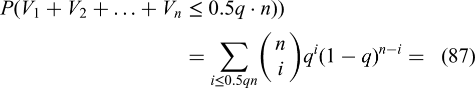
Then, for all

n > 0

, we have:

P (V_{1} + V_{2} + \dots + V_{n} \leq 0.5 q \cdot n) \leq \exp (- 0.025 q \cdot n) .

Proof.

Let $x > 0$ be such that

x \leq 0.25

(85)

We have

1 = (1 + x) (1 - x) + x^{2}

leading to

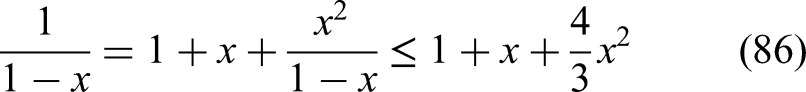
\frac{1}{1 - x} = 1 + x + \frac{x^{2}}{1 - x} \leq 1 + x + \frac{4}{3} x^{2}

(86)

where to obtain the very last inequality above we used (85). We have

P (V_{1} + V_{2} + \dots + V_{n} \leq 0.5 q \cdot n)) = \sum_{i \leq 0.5 q n} (\begin{matrix} n \\ i \end{matrix}) q^{i} (1 - q)^{n - i} =

(87)

= \sum_{i \leq 0.5 q n} (\begin{matrix} n \\ i \end{matrix}) (0.5 q)^{i} \cdot (1 - 0.5 q)^{n - i} \cdot \frac{q^{i} (1 - q)^{n - i}}{(0.5 q)^{i} \cdot (1 - 0.5 q)^{n - i}} \leq

(88)

\leq \sum_{i \leq 0.5 q n} (\begin{matrix} n \\ i \end{matrix}) (0.5 q)^{i} \cdot (1 - 0.5 q)^{n - i} \cdot \frac{q^{0.5 q n} (1 - q)^{n - 0.5 q n}}{(0.5 q)^{0.5 q n} \cdot (1 - 0.5 q)^{n - 0.5 q n}}

(89)

where to obtain the very last inequality above we used the fact that the map

N \to R i \mapsto f (i) = \frac{q^{i} (1 - q)^{n - i}}{(0.5 q)^{i} \cdot (1 - 0.5 q)^{i}}

is increasing. Indeed,

\frac{f (i + 1)}{f (i)} = 2 \frac{1 - 0.5 q}{1 - q} \geq 2.

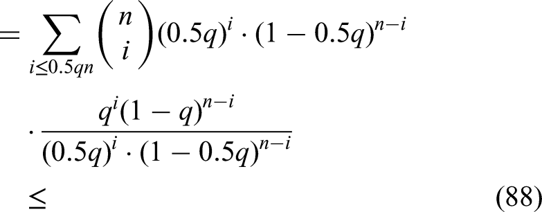
Hence, on the interval

[0, 0.5 q n]

we have that

f (i)

is maximal for

i = 0.5 q n

. This allowed as to obtain inequality (89), by replacing

f (i)

f (0.5 q n)

in (88). Now, note that

\sum_{i \leq 0.5 q n} \begin{matrix} n \\ i \end{matrix} (0.5 q)^{i} \cdot (1 - 0.5 q)^{n - i}

(90)

is the probability that a Binomial Variable with parameters

0.5 q

and

n

be less than

0.5 n q

. Hence, being a probability, expression (90) is less or equal to

1

. Hence, in (89), we can replace (90) by

1

and get the following upper bound:

P (V_{1} + V_{2} + \dots + V_{n} \leq 0.5 q \cdot n)) \leq \frac{q^{0.5 q n} (1 - q)^{n - 0.5 q n}}{(0.5 q)^{0.5 q n} \cdot (1 - 0.5 q)^{n - 0.5 q n}} = {[2^{0.5 q} {(\frac{1 - q}{1 - 0.5 q})}^{1 - 0.5 q}]}^{n}

(91)

We can now apply inequality (86) for

x = 0.5 q

to find

\frac{1 - q}{1 - 0.5 q} \leq (1 - q) (1 + 0.5 q + \frac{1}{3} q^{2}) \leq 1 - 0.5 q .

Applying this to the right side of (91) and taking the logarithm, we find

\ln (P (V_{1} + V_{2} + \dots + V_{n} \leq 0.5 q \cdot n)) \leq n \cdot [0.5 q \cdot \ln (2) + \ln (1 - 0.5 q) \cdot (1 - 0.5 q)] .

The last inequality above, together with the fact that

\ln (1 - Δ) \leq - Δ

implies finally:

\ln (P (V_{1} + V_{2} + \dots + V_{n} \leq 0.5 q \cdot n)) \leq 0.5 q n \cdot [\ln (2) - 1 + 0.5 q)] .

(92)

Now, since we assumed that

q \leq 0.5

, we have that

\ln (2) - 1 + 0.5 q \leq - 0.05

which, when applied to (92), finally yields:

P (V_{1} + V_{2} + \dots + V_{n} \leq 0.5 q \cdot n) \leq \exp (- 0.025 q \cdot n) .

Lemma 3

Assume that $r, l >$ are two natural numbers so that $l \leq 2 r$ . Then,

P (| N_{2 k}^{1} - N_{2 k}^{- 1} | \leq l | N_{2 k}^{1} + N_{2 k}^{- 1} \geq 2 r) \leq 2 l \cdot \frac{\exp (\frac{1}{24})}{\sqrt{r} \sqrt{π}} .

Proof.

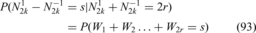
Next note that conditional on $N_{2 k}^{- 1} + N_{2 k}^{- 1} = 2 r$ , we have that $N_{2 k}^{+ 1}$ is a binomial variable with parameters $0.5$ and $2 r$ and same thing for $N_{2 k}^{- 1}$ . To understand why, consider the definition of $N_{2 k}^{+ 1}$ and $N_{2 k}^{- 1}$ : we had $N_{2 k}^{+ 1}$ is the number of indices $i = 1, 2, \dots, 2 k$ for which $X_{i} - X_{i} * = 1$ and similarly $N_{2 k}^{- 1}$ is the number of indices $i = 1, 2, \dots, 2 k$ for which $X_{i} - X_{i} * = 1$ . We could first determine (simulate), which of the indices $i$ are such that $X_{i} - X_{i} *$ are $1$ or $- 1$ : that would yield the number $N_{2 k}^{1} + N_{2 k}^{- 1}$ . Then every index $i$ for which $X_{i} - X_{i} * \in {1, - 1}$ is given, has a probability of $0.5$ to have $X_{i} - X_{i} * = 1$ (conditional probability given $X_{i} - X_{i} * \in {1, - 1}$ ) and the same thing for $X_{i} - X_{i} * = - 1$ . Now the probability to have $1$ or $- 1$ is

P (X_{i} - X_{i} * \in {1, - 1}) = q = 2 p \cdot (1 - p),

we designate that probability by

q

. So,

N_{2 k}^{1} + N_{2 k}^{- 1}

is the number of indexes

i = 1, 2, \dots, 2 k

for which

X_{i} - X_{i} * \in {1, - 1}

holds. Conditional on

N_{2 k}^{1} + N_{2 k}^{- 1} = r

the difference

N_{2 k}^{1} - N_{2 k}^{- 1}

behaves like the position of a symmetric random walk after

2 r

steps:

P (N_{2 k}^{1} - N_{2 k}^{- 1} = s | N_{2 k}^{1} + N_{2 k}^{- 1} = 2 r) = P (W_{1} + W_{2} \dots + W_{2 r} = s)

(93)

where

W_{1}, W_{2}, \dots

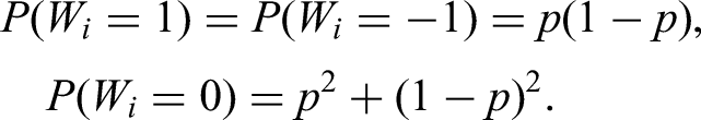
are i.i.d. variable with

P (W_{i} = 1) = P (W_{i} = - 1) = 0.5

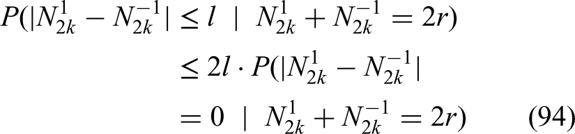
The probabilities of

N_{2 k}^{1} - N_{2 k}^{- 1}

decreases as one moves away from

0

(because binomial varialbw probability decreases when moving away from expectation), so that:

P (| N_{2 k}^{1} - N_{2 k}^{- 1} | \leq l | N_{2 k}^{1} + N_{2 k}^{- 1} = 2 r) \leq 2 l \cdot P (| N_{2 k}^{1} - N_{2 k}^{- 1} | = 0 | N_{2 k}^{1} + N_{2 k}^{- 1} = 2 r)

(94)

According to Lemma 112 however, we have

P (W_{1} + W_{2} + \dots + W_{2 r} = 0) \leq \frac{\exp (\frac{1}{24})}{\sqrt{r} \sqrt{π}} .

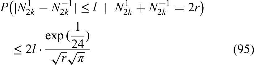
We can apply that last inequality above with (93) and (94), to obtain

P (| N_{2 k}^{1} - N_{2 k}^{- 1} | \leq l | N_{2 k}^{1} + N_{2 k}^{- 1} = 2 r) \leq 2 l \cdot \frac{\exp (\frac{1}{24})}{\sqrt{r} \sqrt{π}}

(95)

Noting that the bound on the right side of the very last inequality above decreases in

r

, we find:

P (| N_{2 k}^{1} - N_{2 k}^{- 1} | \leq l | N_{2 k}^{1} + N_{2 k}^{- 1} \geq 2 r) \leq 2 l \cdot \frac{\exp (\frac{1}{24})}{\sqrt{r} \sqrt{π}}

(96)

which finishes this proof!

Lemma 4

For any integer $t > 0$ , Assume we chose in the integer interval $[1, k]$ a subset $Δ_{k}^{t}$ of size $t < k$ at random, with equal probability among all subsets of that size. Then, we chose independently two additional integer points ${\tilde{Z}}_{1}$ and ${\tilde{Z}}_{2}$ from the interval $[1, k]$ , with equal probability among all the points. (The random variables ${\tilde{Z}}_{1}$ and ${\tilde{Z}}_{2}$ are independent of each other and of the set $Δ_{k}^{t}$ ). Let $H_{k}^{t}$ be the event that there are at least three points of $Δ_{k}^{t}$ , which are larger or equal to $max ({\tilde{Z}}_{1}, {\tilde{Z}}_{2})$ . Then,

P (H_{k}^{t}) \geq 1 - \frac{4}{t} .

Proof.

For $i = 0, 1, 2$ , let $D_{i}$ be the event that exactly $i$ of the two points $Z_{1}, Z_{2}$ are the integer set $Δ_{k}^{t}$ . Given that $D_{2}$ holds, so both ${\tilde{Z}}_{1},$ and ${\tilde{Z}}_{2}$ are in $Δ_{k}^{t}$ , we have that ${\tilde{Z}}_{1}, {\tilde{Z}}_{2}$ can be any of the points in $Δ_{k}^{t}$ . In other words, once we have determined the set $Δ_{k}^{i}$ , then which of these points is ${\tilde{Z}}_{1}$ and which is ${\tilde{Z}}_{2}$ is obtained by choosing at random with equal probability among the points of $Δ_{k}^{t}$ . So, when $B_{2}$ holds, for the event $H_{k}^{t}$ to hold, we simply need none of the points ${\tilde{Z}}_{1}$ and ${\tilde{Z}}_{2}$ to be equal to the two biggest points of the set $Δ_{k}^{t}$ . This has a probability: $[(t - 2) / t]^{2}$ , so that we find

P (H_{k}^{t} | D_{2}) = {[\frac{t - 2}{t}]}^{2} = {(1 - \frac{2}{t})}^{2} = 1 - \frac{4}{t} + \frac{4}{t^{2}} \geq 1 - \frac{4}{t} .

(97)

Assume next, that exactly one of the points

{\tilde{Z}}_{1}, {\tilde{Z}}_{2}

is in the set

Δ_{k}^{t}

, so that the event

D_{1}

holds. Then we can consider the set

Δ_{k}^{t} \cup {Z - 1, Z_{2}}

(98)

which has size

t + 1

, when

D_{1}

holds. Having determined, that set (98), any two points are equally likely to be the points

Z_{1}

and

Z_{2}

. Hence to get

H_{k}^{t}

to hold, we need the two points not be equal to the two biggest points of that set with size

t + 1

, hence

P (H_{k}^{t} | D_{1}) = {[\frac{t - 1}{t + 1}]}^{2} = {[1 - \frac{2}{t + 1}]}^{2} \geq 1 - \frac{4}{t + 1}

(99)

Finally, when

D_{0}

holds, then the set given in (98) has size

t + 2

leading to the inequality

P (H_{k}^{t} | D_{0}) \geq 1 - \frac{4}{t + 2} .

(100)

We can now use the Law of Total Probability together with the inequalities (97), (99) and (100),to find:

\begin{aligned} P (H_{k}^{t}) = & P (H_{k}^{t} | D_{2}) \cdot P (D_{2}) + P (H_{k}^{t} | D_{1}) \cdot P (D_{1}) + P (H_{k}^{t} | D_{0}) \cdot P (D_{0}) \geq \\ \geq & (1 - \frac{4}{t}) \cdot P (D_{2}) + (1 - \frac{4}{t + 1}) \cdot P (D_{1}) + (1 - \frac{4}{t + 2}) \cdot P (D_{2}) \geq \\ \geq & (1 - \frac{4}{t}) \cdot P (D_{2}) + (1 - \frac{4}{t}) \cdot P (D_{1}) + (1 - \frac{4}{t}) \cdot P (D_{2}) = \\ = 1 - \frac{4}{t} . \end{aligned}

Hence,

P (H_{k}^{t}) \geq 1 - \frac{4}{t},

which finishes this proof.

Lemma 5

Let $H_{k}$ be the event that there are at least three points of $Δ_{k}$ , which are larger or equal to $max (Z_{1} *, Z_{2} *)$ . Then, we have

P (H_{k} ‖ Δ_{k} | = l) \geq 1 - {0.99}^{l} - \frac{10}{l} .

Proof.

Let us divide the integer interval $[1, 2 k]$ into two subsets $I_{s m a l l}$ and $I_{l a r g e}$ of equal size $k$ each. Furthermore, this partition of $[1, 2 k]$ into $I_{s m a l l}$ and $I_{l a r g e}$ is done to separate the larger coefficients $a_{i}$ from the smaller ones. More precisely,, we assume that for all $i, j \in [1, 2 k]$ if $i \in I_{s m a l l}$ and $j \in I_{}$ , then

a_{i} \leq a_{j} .

Recall, that the points

\tilde{Z} *_{1}

and

{\tilde{Z}}_{2} *

are chosen at random from the set

I_{l a r g e}

Let $C_{k}$ be the event that among the points of the random sets $Δ_{k}$ at least $40 %$ are in the interval $I_{l a r g e}$ . Note that

H_{k} \cap C_{k} \subset H_{k},

hence

P (H_{k} | | Δ_{k} | = l) \geq P (H_{k} \cap C_{k} |, : | Δ_{k} | = l) =

(101)

= P (H_{k} | C_{k} \cap {| Δ_{k} = l}) \cdot P (C_{k} | | Δ_{k} | = l)

(102)

Now, when

C_{k}

holds, then at least

40 %

of the points of

Δ_{k}

are in

I_{l a r g e}

. So, when

| Δ_{k} | = l

holds, that means that there are at least

0.4 \cdot l

points of the random set

Δ_{k}

in the interval

I_{l a r g e}

. In that case, the event

H_{k}

happens every time there are least

3

of these

0.4 \cdot l

points which are larger than

Z_{1} *, Z_{2} *

. This corresponds to the event

H_{k}^{t}

with

t = 0.4 l

. (Note the event

H_{k}^{t}

was defined for a random subset of size

t

from

[1, k]

, but the same probability must hold when we have the same problem for a random subset from the integer interval

I_{l a r g e}

and size

t = 0.4 l

] ). Hence, we get the bound:

P (H_{k} | C_{k} \cap {| Δ_{k} | = l}) \geq P (H_{k}^{0.4 \cdot l})

(103)

The event on the right side of the inequality above can be bounded thanks to the previous Lemma, so that

P (H_{k}^{0.4 \cdot l}) \geq 1 - \frac{10}{l}

(104)

Now, the probability of a random integer points chosen at random in the interval

[1, 2 k]

to be within the interval

I_{l a r g e}

0.5

. So, by large deviation to have only

40 %

of the random points of

Δ_{k}

I_{l a r g e},

instead of about

50 %

is exponentially negatively small in the size of

Δ_{k}

. To get a bound, consider:

Let $W_{1}, W_{2}, \dots$ be i.i.d. Bernoulli variable with

P (W_{i} = 1) = P (W_{i} = 0) = 0.5

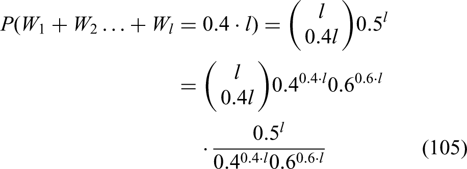
Now, we want to bound the probability to get

40 %

1

’s, instead of

50 %

P (W_{1} + W_{2} \dots + W_{l} = 0.4 \cdot l) = (\begin{matrix} l \\ 0.4 l \end{matrix}) {0.5}^{l} = (\begin{matrix} l \\ 0.4 l \end{matrix}) {0.4}^{0.4 \cdot l} {0.6}^{0.6 \cdot l} \cdot \frac{{0.5}^{l}}{{0.4}^{0.4 \cdot l} {0.6}^{0.6 \cdot l}}

(105)

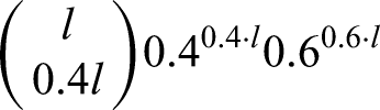
Now, the expression:

(\begin{matrix} l \\ 0.4 l \end{matrix}) {0.4}^{0.4 \cdot l} {0.6}^{0.6 \cdot l}

is the probability that a binomial variable with parameters

0.4

and

l

takes on the value

0.4 l

. Hence, it is less than or equal to

1

. Together with equation (105), this implies

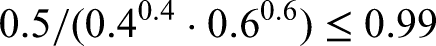
P (W_{1} + W_{2} \dots + W_{l} = 0.4 \cdot l) \leq \frac{{0.5}^{l}}{{0.4}^{0.4 \cdot l} {0.6}^{0.6 \cdot l}}

(106)

Now, the number

0.5 / ({0.4}^{0.4} \cdot {0.6}^{0.6}) \leq 0.99

so that the right side of (106) is bounded by

{0.99}^{l}

yielding:

P (C_{k} | | Δ_{k} | = l) \geq 1 - {0.99}^{l} .

(107)

(One should note that we showed the bound 106 for the probability to be exactly equal to

0.4 l

rather than less or equal to

0.4 l

. However, the same bound also holds for less or equal to

0.4 l

, and the proof is very similar using the same technique as in the proof of Lemma (2) So, together inequalities (101), (102), (103) and (104) imply

P (H_{k} | | Δ_{k} | = l) \geq 1 - \frac{10}{l} - {0.99}^{l} .

(108)

Simulations

In this article, we investigate how tightly we can bound the probability of the symmetric difference between the events $A$ and $B$ . Specifically, we aim to determine how small the constant $ϵ > 0$ can be in the inequality

P (A - B) + P (B - A) \leq ϵ P (A) .

(109)

The main results of this article is presented in Theorem 1 is a lower bound for such

ϵ > 0

satisfying (109). Note that the expression on the left side of (109) is equal to the expected sum of squared differences between the corresponding indicator functions:

E [(1_{A} - 1_{B})^{2}] .

Here, the indicator function

1_{A}

is equal to

1

when the event

A

holds, and

1_{A} = 0

otherwise. Similarly,

1_{B} = 1

when

B

holds, and

1_{B} = 0

otherwise. In the context of this paper, the event

A

is given, but for

B

B = {a_{1} X_{1} + a_{2} X_{2} + \dots + a_{2 k} X_{k} \geq c},

we try to determine coefficients

a_{1}, a_{2}, \dots, a_{2 k}, c

so as to approximate

1_{A}

as closely as possible. When we try to approximate

1_{A}

as closely as possible with

1_{B}

, we are dealing with the Perceptron algorithm with one Neuron. The original Perceptron algorithm is only guaranteed to work when the data is linearly separable, which is not the case here. Gradient descent would not work here, since the Heaviside function

h (.)

1_{B} = h (a_{1} X_{1} + a_{2} X_{2} + \dots + a_{2 k} X_{k} - c),

(110)

is not continuous at

x = 0

. (Here

h (x) = 1

for

x \geq 0

and

h (x) = 0

for

x < 0

). For our simulations, instead of Heaviside, we will use the Sigmoid function:

σ (x) = \frac{1}{1 + e^{- x}},

which takes values between

0

and

1

. Henceforth, instead of approximating

1_{A}

by (110), we approximate it by

σ (a_{1} X_{1} + a_{2} X_{2} + \dots + a_{2 k} X_{k} - c) .

(111)

The closest approximation possible in terms of expected Sum of Squared Error is a lower bound to the expected Sum of Squared error of the approximation with

1_{B}

. The reason is that the Heaviside function can be approximated arbitrarily closely by the Sigmoid function:

lim_{a \to + \infty} σ (x \cdot a) = h (x)

for all

x \neq 0

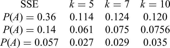
The surprising discovery we made in our simulations, is that for relatively small $k$ , like $k = 5$ and not exceedingly small $P (A)$ , we seem to not be able to go much below $0.5 P (A)$ for the Sum of squared error, rather than our theoretical bound which is asymptotically about $\frac{P (A)}{16}$ . Again, our result is asymptotic, for $k p_{k} \cdot (1 - p_{k})$ converging to infinity and assuming $P (A) << 1$ . However, in the table below we see that gradient descent can not find a solution much below $0.5 P (A)$ in most cases, even for values of $P (A)$ which are not very small and $k$ which is not very large! Also, we had no doubt that the result would hold for large k, since the Central Limit Theorem would apply in that case. But, in applications like a chat-bot, the implications often contain between $5$ and $10$ arguments. We see in the simulations below that our lower bound already applies with that order of magnitude. This implies that the current result also applies to real-life applications. Let us see our numeric results for Sum of Squared Error for approximating $1_{A}$ with the Sigmoid given in (111). Hence, the following table contains the value

SSE = min_{a_{1}, a_{2}, \dots, a_{2 k}, c} E [{(1_{A} - σ (a_{1} X_{1} + a_{2} X_{2} + \dots + a_{2 k} X_{k} - c))}^{2}] .

The table is for different values of

k

and

P (A)

\begin{matrix} SSE & k = 5 & k = 7 & k = 10 \\ P (A) = 0.36 & 0.114 & 0.124 & 0.120 \\ P (A) = 0.14 & 0.061 & 0.075 & 0.0756 \\ P (A) = 0.057 & 0.027 & 0.029 & 0.035 \end{matrix}

When we now calculate the ration $SSE / P (A)$ from the table above, we get a lower bound for $ϵ > 0$ satisfying (109) and depending on $k$ and $P (A)$ :

\begin{matrix} SSE / P (A) & k = 5 & k = 7 & k = 10 \\ P (A) = 0.36 & 0.31 & 0.34 & 0.33 \\ P (A) = 0.14 & 0.43 & 0.53 & 0.54 \\ P (A) = 0.057 & 0.47 & 0.50 & 0.61 \end{matrix}

Our theoretical bound is

1 / 16

, but in the last table above we are mostly close to

0.5

. This would correspond to our heuristic argument given at the beginning of the proof of Theorem 1, which used as assumption the holding of the CLT, which may not always be the case. Seeing the values in the last table above, we believe that the heuristic argument presented at the beginning of the proof of Theorem 1, which implied a lower bound approximately equal to

0.5

, seems to apply quite well for practical situations.

Footnotes

ORCID iD

Heinrich Matzinger

Funding

The authors received no financial support for the research, authorship and/or publication of this article.

Appendix

References

Zoph

Bello

Kumar

et al. Designing effective sparse expert models. arXiv preprint arXiv:220208906 2022.

Komatsuzaki

Puigcerver

Lee-Thorp

et al. Sparse Upcycling: Training Mixture-of-Experts from Dense Checkpoints. arXiv e-prints 2022; arXiv:2212.05055.

Shazeer

Mirhoseini

Maziarz

et al. Outrageously large neural networks: The sparsely-gated mixture-of-experts layer. arXiv preprint arXiv:170106538 2017.

Vaswani

Shazeer

Parmar

et al. Attention is all you need. In Guyon

Luxburg

Bengio

et al. (eds.) Advances in Neural Information Processing Systems, volume 30. Curran Associates, Inc. https://proceedings.neurips.cc/paper_files/paper/2017/file/3f5ee243547dee91fbd053c1c4a845aa-Paper.pdf.

Sharma

Kaplan

. Scaling laws from the data manifold dimension. J Mach Learn Res 2022; 23(1): 343–376.

Gordon

Duh

Kaplan

. Data and parameter scaling laws for neural machine translation. In Proceedings of the 2021 Conference on Empirical Methods in Natural Language Processing. pp. 5915–5922.