
Abstract
Background:
Spike-and-wave activation in sleep (SWAS) may lead to irreversible cognitive impairment, progressing to epileptic encephalopathy (EE)-SWAS. However, existing EEG studies have not differentiated between SWAS patients based on their future cognitive outcomes.
Objectives:
This study aims to extract features from the sleep EEG of SWAS patients and develop a machine learning model to predict cognitive outcomes.
Design:
A retrospective study.
Methods:
A retrospective analysis was conducted on the sleep EEG obtained during the interictal period of 41 SWAS patients (15 with cognitive impairment). Cognitive impairment prediction models (support vector machine (SVM) and light gradient boosting machine (LightGBM)) were constructed based on spike-wave index (SWI) (the gold standard for diagnosing SWAS) and multidimensional EEG features, including functional connectivity (FC), minimum spanning tree (MST), and time–frequency-nonlinear (TFN) features, alongside a multidomain fusion (MDF) model integrating all feature sets. The performance of these EEG-based models was compared with the SWI model.
Results:
Models using the single SWI feature showed limited predictive capability (highest ACC: 0.756, AUC: 0.749). Conversely, multidimensional EEG models demonstrated superior performance. Specifically, the FC-based SVM model achieved the highest accuracy (0.873). Furthermore, MDF-based LightGBM models outperformed all single-feature-set models in overall discriminative capability (highest AUC: 0.934). These findings highlight the superiority of multidimensional EEG features over SWI for predicting cognitive outcomes in SWAS.
Conclusion:
The developed EEG-based machine learning models hold potential to assist in early cognitive prediction and treatment decisions for SWAS patients. However, given the current methodological limitations, further clinical verification is warranted.
Keywords
Introduction
Developmental and epileptic encephalopathy (DEE) and epileptic encephalopathy (EE) with spike-and-wave activation in sleep (SWAS) are characterized by seizure onset between 2 and 12 years of age (peaking at 4–5 years). Approximately 1–2 years after the initial seizures, the EEG of these patients develops spike-and-wave activation in sleep, which is closely associated with cognitive or behavioral regression or plateauing. 1 The EEG pattern associated with SWAS is referred to as electrical status epilepticus in sleep (ESES). Although SWAS frequently remits during adolescence, the related cognitive impairments are often irreversible. 2 Early suppression of pathological discharges has been shown to alleviate cognitive decline and improve prognosis, whereas delayed diagnosis or treatment increases the risk of long-term disability. 3 However, early cognitive regression is often subtle and difficult to detect, leading some patients to miss the optimal window for intervention. Moreover, in an effort to prevent disease progression, some clinicians initiate treatment aggressively regardless of the presence of cognitive or behavioral regression, 4 which may result in overtreatment and consequently lead to unnecessary drug-related side effects, thereby increasing the risk of medication-induced cognitive impairment. 5 Therefore, there is an urgent need for a rapid and objective method to accurately predict cognitive impairment at the early stage of SWAS detection, thereby providing a basis for precision treatment planning.
Machine learning has emerged as a powerful approach for pattern recognition and classification based on multidimensional features and has been increasingly applied to neurological disorders, including SWAS. For example, Meng et al. employed a graph convolutional neural network based on Chebyshev polynomials for ESES detection, which could automatically and accurately distinguish between ESES and non-ESES activities, achieving an accuracy of 91.2%. 6 Chavakula et al. combined a dual-threshold wavelet transform with machine learning algorithms to automatically quantify spikes in raw EEG samples of ESES patients. 7 Rein et al. used a LASSO regression model with an elastic net to predict whether patients with benign epilepsy with centrotemporal spikes (BECTS) would progress to ESES. 8 However, effective approaches for the early prediction of cognitive impairment in SWAS patients remain lacking. This gap limits the ability of clinicians to identify high-risk individuals upon the initial detection of SWAS, leading to delayed intervention or unnecessary overtreatment. Therefore, developing an early prediction model for cognitive impairment in SWAS may provide a valuable tool for precision assessment and intervention of SWAS-related cognitive impairment.
The exact mechanisms underlying the abnormal cortical activation observed in SWAS remain unclear, and the pathways through which sleep influences cognition have not been systematically elucidated. Nevertheless, several studies have provided insights from different perspectives. He et al., using resting-state fMRI, found that children with BECTS accompanied by ESES exhibited markedly reduced functional connectivity (FC) within the salience and central executive networks during sleep, while the default mode network remained relatively preserved. 9 This network imbalance may disrupt information integration and executive control during sleep, thereby contributing to cognitive impairment. Van den Munckhof et al. analyzed overnight EEG recordings and reported a reduced nocturnal decline in slow-wave slope within epileptogenic regions, which correlated with the severity of behavioral problems. 10 These findings suggest that epileptic activity may interfere with synaptic homeostasis and consequently affect cognitive function. Wodeyar et al. further demonstrated, through simultaneous human thalamo-cortical recordings, that epileptic spikes can “hijack” thalamo-cortical loops, suppressing the generation of sleep spindles that are essential for memory consolidation, thereby directly impairing cognition. 11 Although these studies consistently indicate a close association between sleep-related epileptiform activity and cognitive impairment in SWAS, no studies have stratified patients based on their longitudinal cognitive outcomes. This study categorizes SWAS patients according to whether they subsequently developed cognitive impairment, and aims to uncover the underlying mechanisms through feature analysis using EEG-based machine learning methods.
Sleep EEG recordings obtained during the interictal period at the early stage of SWAS detection from 41 patients with SWAS were analyzed. Three categories of features were extracted, including functional connectivity (FC), minimum spanning tree (MST), and time–frequency-nonlinear (TFN) features. Furthermore, a multidomain fusion (MDF) feature set was constructed by integrating all the extracted features. Support vector machine (SVM) and light gradient boosting machine (LightGBM) models were then constructed to predict future cognitive outcomes in SWAS patients, aiming to facilitate early identification of high-risk individuals and to inform precision intervention strategies.
Materials and methods
Participants
This study included pediatric patients diagnosed as epilepsy with SWAS who underwent TCD-vEEG at Guangzhou Women and Children’s Medical Center (Guangzhou, China) between August 2017 and March 2022, with a minimum follow-up period of 6 months postexamination. Inclusion criteria were a spike-wave index (SWI) >50% during nonrapid eye movement (NREM) sleep persisting for over 1 year (without SWI variation during follow-up) and IED distribution in bilateral or multifocal patterns. Exclusion criteria were the occurrence of clinical epileptic seizures during the video-EEG recording, continuous artifacts in EEG, difficulties in cognitive function assessment, developmental delay or intellectual disability prior to seizure onset, and significant structural abnormalities on cranial MRI. We have followed the Strengthening of the Reporting of Observational Studies in Epidemiology (STROBE) guidelines when preparing this manuscript (Supplemental Material).
Patients were categorized into the cognitive impairment group (CIG) and the without cognitive impairment group (WCIG). Cognitive impairment was assessed using a combination of neuropsychological testing (Wechsler Intelligence Scale for Children Chinese Version IV (WISC-IV)) and parental reports on the child’s language, learning, and motor abilities. All included patients exhibited normal cognitive function at the time of the EEG acquisition. Group assignment was determined strictly based on longitudinal follow-up outcomes (with a minimum follow-up period of 6 months). Patients who demonstrated cognitive regression (e.g., IQ/DQ scores falling below 70) during the follow-up period were assigned to the CIG, whereas those who maintained normal cognitive function were assigned to the WCIG.
Clinical features
Clinical data collected included demographic information (age, sex, age at first seizure), disease course, seizure type and frequency, etiology, previous psychomotor development, cognitive function assessments, language ability, academic performance during follow-up, and intelligence assessments. Additional information on febrile convulsions, antiseizure medications (ASMs), other treatments, EEG findings, brain MRI results, and final diagnosis was also documented.
EEG acquisition and preprocessing
The overall analytical pipeline is summarized in Figure 1.
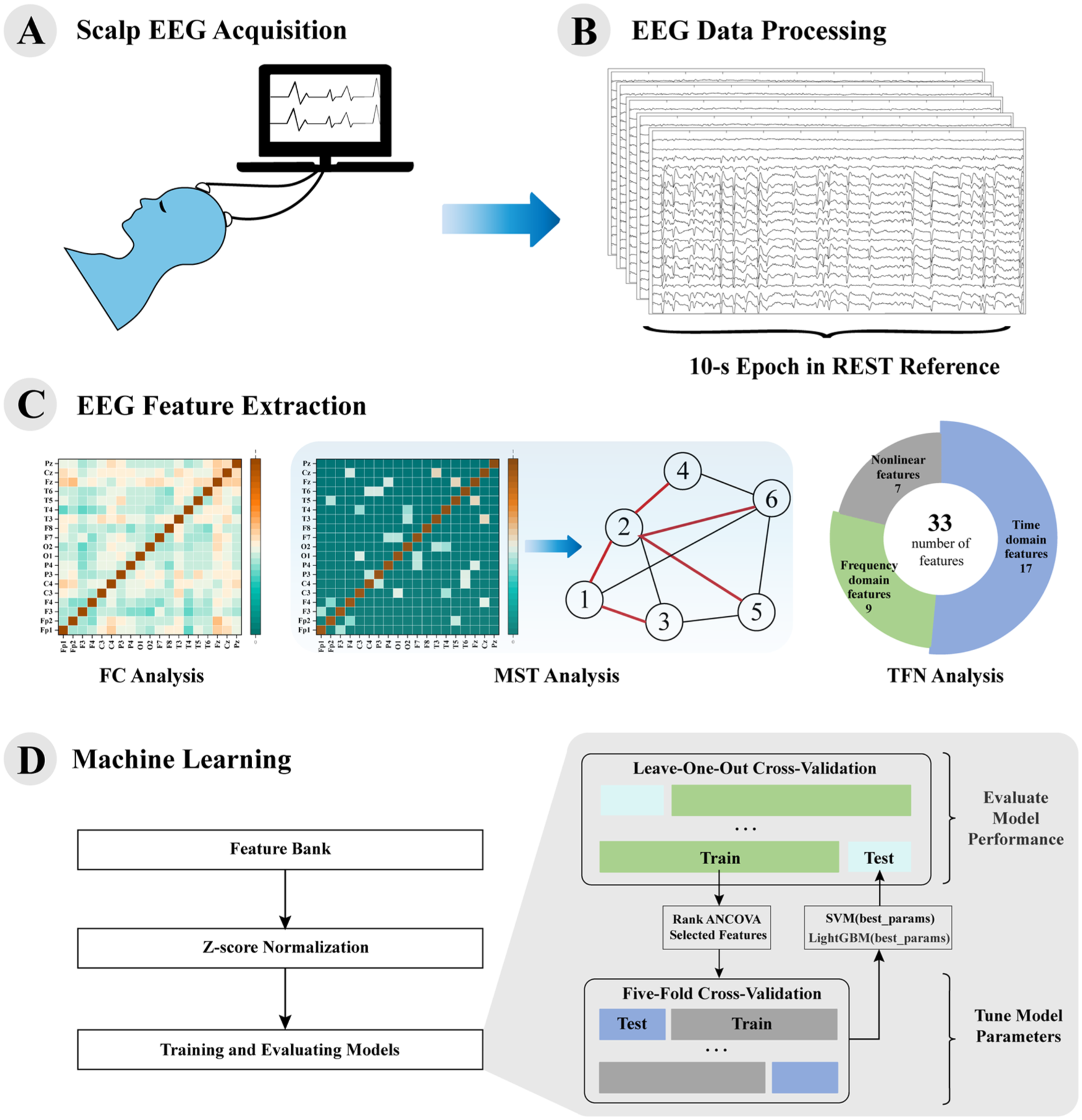
(a) Scalp EEG recording from 15 patients with cognitive impairment and 26 patients without cognitive impairment. (b) Preprocessed EEG segmented into ten 10-s REST reference epochs. (c) EEG feature extraction with FC, MST, and TFN features. (d) Machine learning flowchart, using both SVM and LightGBM models.
Following a sleep-deprived vEEG (SD-vEEG) protocol, participants were allowed to sleep in a quiet, semi-dark room without external stimulation. Simultaneous EEG and video recording was performed using a digital EEG polygraph (NicoletOne EEG, Natus, USA). Scalp electrodes (19 in total) were applied according to the 10–20 system (Electrocap, ECI, OH, USA), with bilateral myoelectric electrodes on the deltoids and bilateral electrooculographic (EOG) electrodes on the face. EOG and EEG data were collected at a sampling rate >1000 Hz. Only EEG data from the 19 electrodes were used for analysis. EMG data were collected at a 1000 Hz sampling rate and filtered between 20 and 200 Hz. vEEG recordings typically lasted over 60 min, with at least 10 min of deep sleep. SWI during sleep was calculated as the proportion of total NREM sleep time containing spike waves. Deep sleep was defined by >20% delta activity in EEG channels, as determined by visual inspection in 30-second epochs according to the American Academy of Sleep Medicine (AASM) manual. 12
EEG data were preprocessed using MATLAB R2020a (MathWorks, Natick, MA, USA) equipped with the EEGLAB toolbox (version 2023.1). Specifically, preprocessing included linear detrending, application of a 50 Hz notch filter to remove powerline interference, downsampling to 512 Hz, independent component analysis (ICA) for artifact removal, and re-referencing.
For artifact correction, ICA was performed using the ICLABEL plugin, 13 which automatically labeled components with <20% brain activity or >90% ocular/muscle activity. The identified artifactual components were further inspected and manually removed (an average of 1.731 ± 1.674 components were removed per subject).
Re-referencing was conducted using the Reference Electrode Standardization Technique (REST), which converts EEG data referenced to scalp or body sites (or to average/linked ears) into data referenced to a theoretical zero-potential at infinity, yielding a reference-free representation of brain potentials. 14
After preprocessing, artifact-free EEG segments were selected. For each patient, ten 10-second epochs with minimal artifacts were extracted, yielding a total of 410 EEG segments for analysis.
EEG feature extraction
Spike-wave index
The SWI is defined as the percentage of NREM sleep occupied by spikes and waves,15,16 and its calculation formula is shown below.
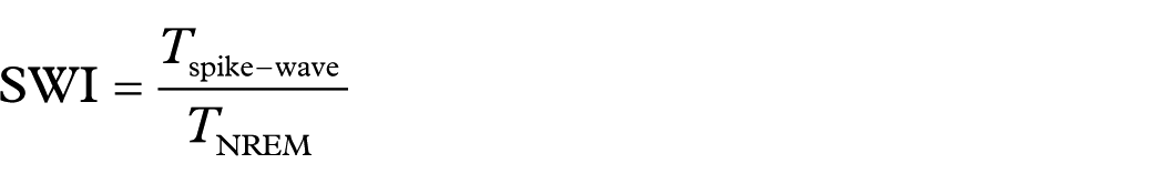
where
FC analysis
The weighted phase lag index (wPLI) is commonly used to estimate the degree of phase synchrony between two signals over time and to quantify the strength of FC between pairs of EEG electrodes. 17 In this study, the instantaneous phase of EEG signals was calculated using the Hilbert transform, and the wPLI was computed as follows:
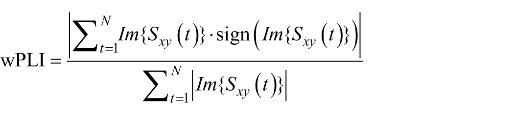
where
Before calculating the wPLI, current source density (CSD) analysis was applied to the EEG data to further minimize the effects of volume conduction (VC). This procedure estimates the radial current flow from underlying neuronal populations at given scalp locations toward the skull and scalp surface, thereby improving the spatial resolution of EEG signals. 18
For each subject, five frequency bands were extracted from each EEG segment: δ (0.5–4 Hz), θ (4–8 Hz), α (8–13 Hz), β (13–30 Hz), and γ (30–80 Hz). The wPLI was computed for every pair of electrodes within each band, which were subsequently used as candidate features.
MST analysis
MST is a subnetwork that connects all nodes while minimizing the total edge weight without forming any cycles. For a fully connected undirected weighted network with distinct edge weights, only one unique MST exists. The MST provides an unbiased approach for brain network analysis, effectively addressing the threshold selection problem inherent in conventional graph-theoretical analyses. 19
The inverse of the wPLI was used as the edge weight, and each EEG electrode was treated as a node. MSTs were constructed for five frequency bands using Kruskal’s algorithm. 20 From each MST, six global metrics were extracted—maximum degree, leaf fraction, diameter, average eccentricity, maximum betweenness centrality, and tree hierarchy—and two local metrics, eccentricity and betweenness centrality, were computed for each node. The definitions of these MST features are summarized in Table 1. Finally, the mean wPLI (MwPLI) of each electrode across all pairs was calculated.
MST features and interpretation.
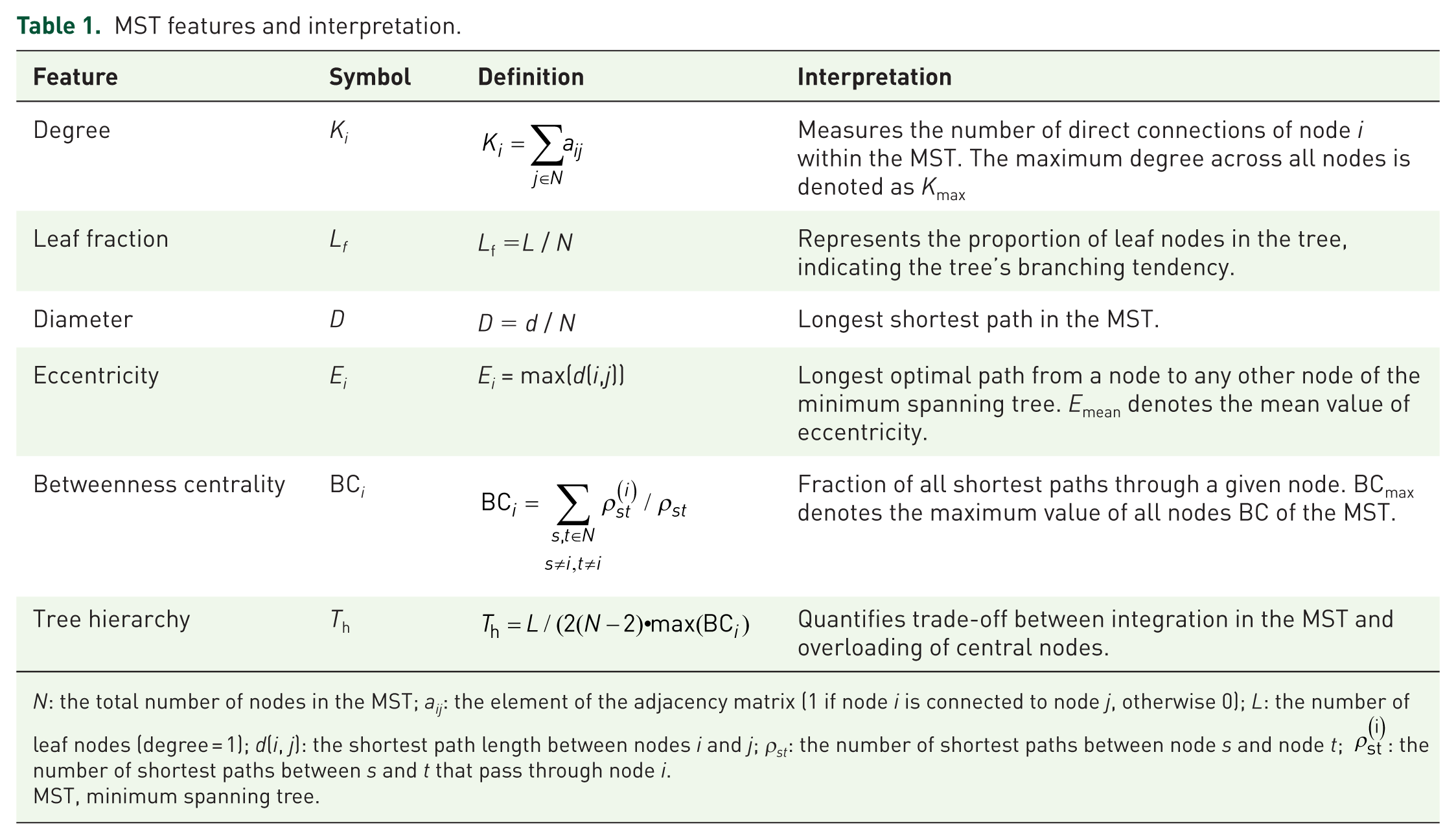
N: the total number of nodes in the MST; a
ij: the element of the adjacency matrix (1 if node i is connected to node j, otherwise 0); L: the number of leaf nodes (degree = 1); d(i, j): the shortest path length between nodes i and j; ρst: the number of shortest paths between node s and node t;
MST, minimum spanning tree.
TFN analysis
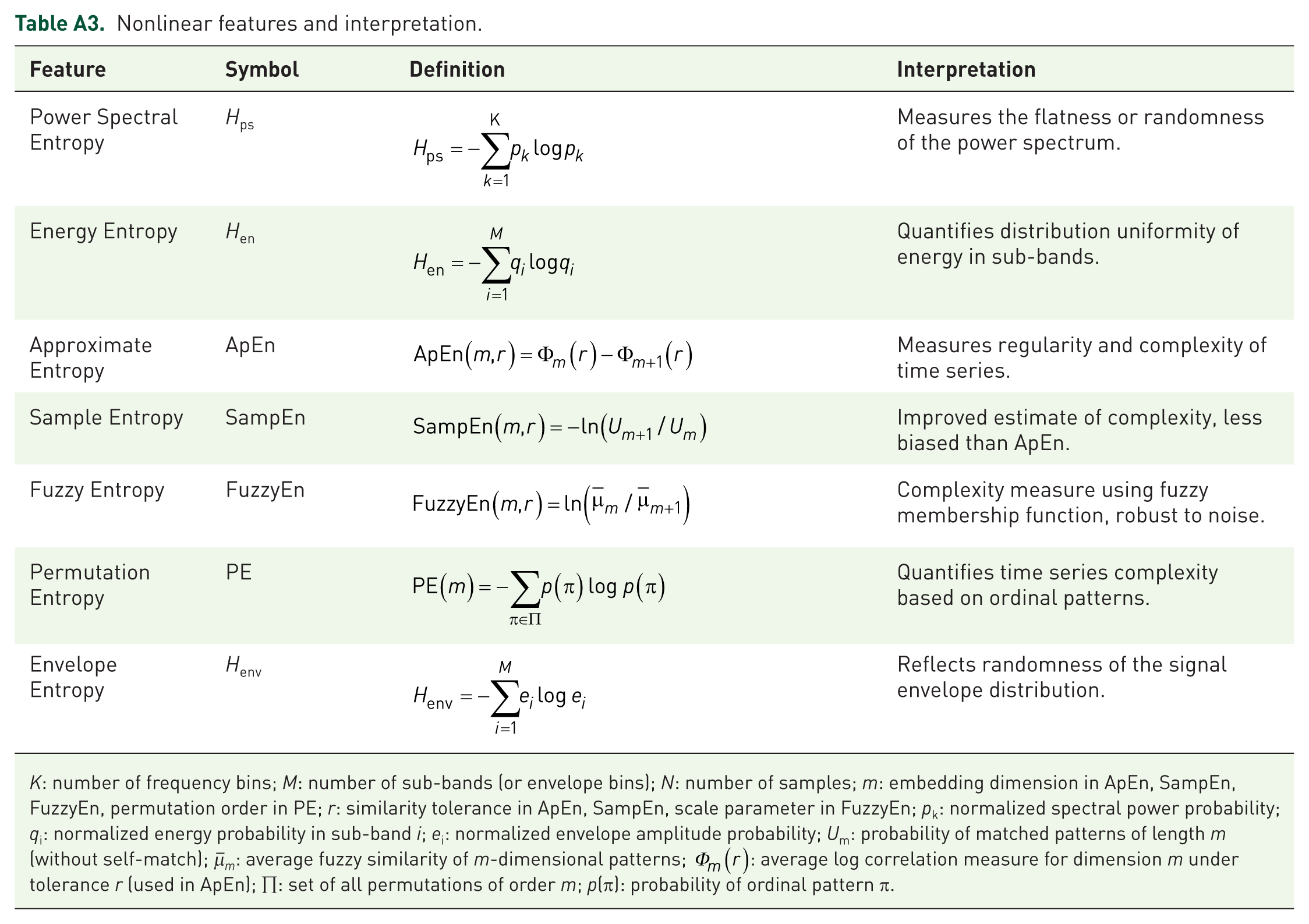
Time-domain, frequency-domain, and nonlinear analytical methods have been widely applied in EEG analysis. However, few studies have incorporated these approaches into the investigation of SWAS. Therefore, in this study, 33 features were extracted across five frequency bands and all EEG channels, encompassing time-, frequency-, and nonlinear-domain characteristics to construct a feature set. The full list of features is provided in Tables A1–A3.
MDF analysis
To evaluate the synergistic effects and overall predictive capacity of different feature domains, all extracted features from the aforementioned sets (SWI, FC, MST, and TFN) were concatenated to construct an MDF feature set for subsequent machine learning analysis.
Machine learning analysis
Two machine learning models—SVM and LightGBM—were used in this study. The SVM constructs an optimal hyperplane in a high-dimensional feature space to maximize the separation margin between two classes. 21 LightGBM, a gradient boosting framework based on decision trees, offers faster computation and higher accuracy compared with other ensemble learning methods. 22
To determine the optimal feature subset and ensure our models capture intrinsic cognitive biomarkers rather than medication signatures, we first incorporated pre-EEG medications with significant differences between groups as covariates into the Rank analysis of covariance (Rank ANCOVA) to rank the features. We employed nested cross-validation: the inner loop used fivefold cross-validation for hyperparameter optimization, while the outer loop utilized leave-one-out cross-validation to assess generalization performance. The entire feature selection process was embedded within the outer loop. During this training process, a class-weight balancing configuration was applied to both models to mitigate potential biases caused by class imbalance. Furthermore, the Nogueira stability measure
Statistical analysis
Statistical analyses were conducted using SPSS 26.0. The D’Agostino–Pearson omnibus normality test was used to evaluate the normality of the features. Continuous variables with normal distribution are presented as mean and standard deviation, while continuous variables with nonnormal distribution are expressed as median and interquartile range. Categorical variables are presented as the frequency and percentage. The differences in continuous variables with a normal distribution between groups were assessed using the independent-samples t-test. Rank analysis of covariance (Rank ANCOVA) was employed to control for the confounding effects of significant medication variables during feature selection. The differences of all analyzed clinical factors between groups were compared and tested using the chi-square test. The strict false discovery rate (FDR) correction based on the Benjamini–Hochberg method was applied to the p-values, and statistical significance was considered for p < 0.05. The final dataset contained no missing values; thus, data imputation was not required.
Results
Clinical features of patients
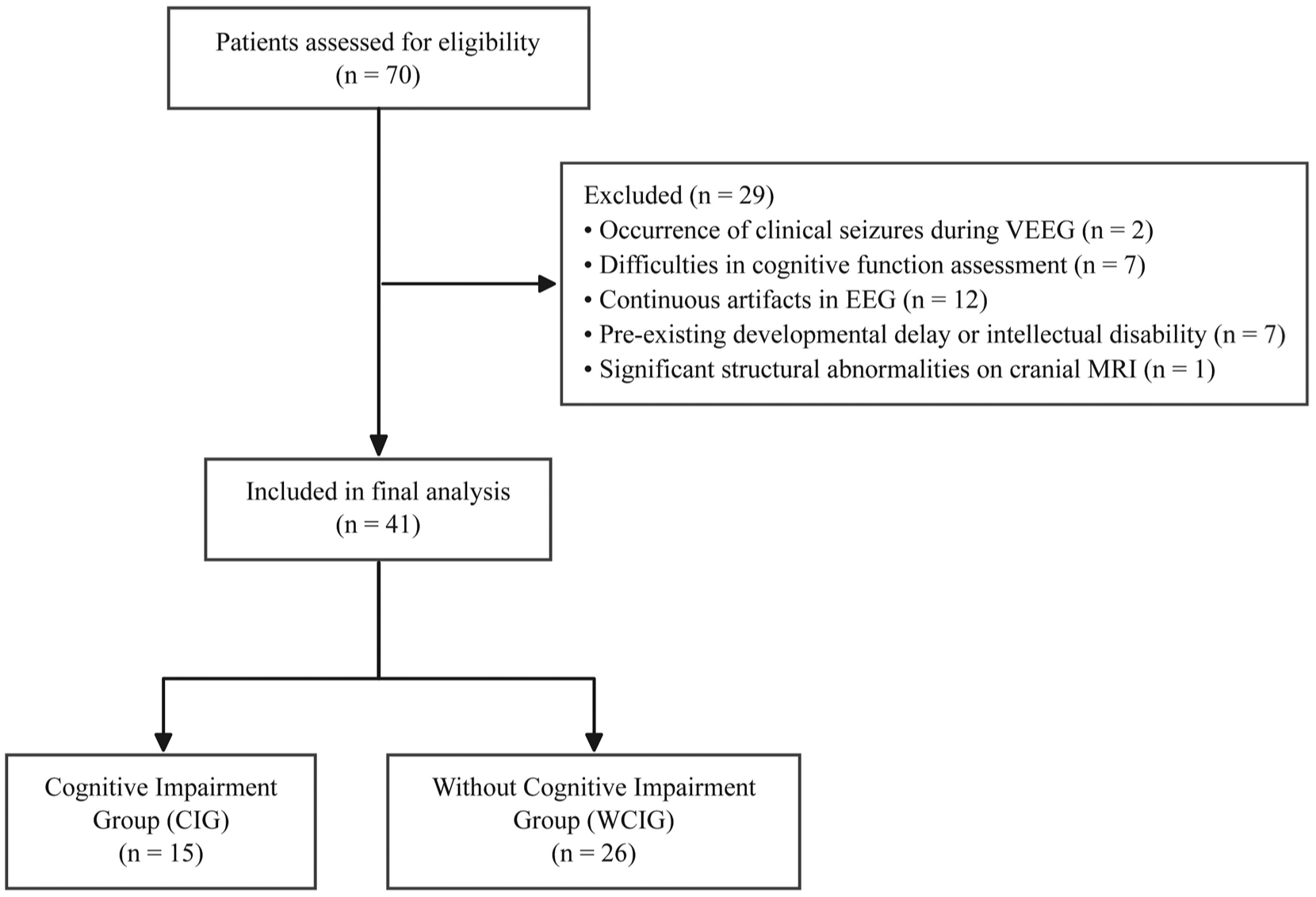
Flow diagram of patient selection. A total of 70 pediatric patients with SWAS were initially assessed for eligibility. After applying the predefined exclusion criteria, 29 patients were excluded. The final cohort consisted of 41 patients, including 15 in the CIG and 26 in the WCIG.
Initially, a total of 70 pediatric patients diagnosed with SWAS were assessed for eligibility. Based on the predefined exclusion criteria, 29 patients were excluded (Figure 2). Consequently, a total of 41 patients (30 males, 11 females; age range 3–13 years) were included in the study. The age of onset ranged from 2 to 10 years. They were followed up in our hospital from half a year to twelve years. Three patients were diagnosed with Landau–Kleffner syndrome (LKS), while the remaining thirty-eight children had focal epilepsy, including four with atypical benign focal epilepsy of childhood (ABFEC); one child accepted surgery; thirty children were diagnosed as self-limited epilepsy with central temporal spikes (SeLECTs); the remaining four cases whose genetic test were negative, remained unclassified. Additionally, 29 patients did not have seizures within the 3 months before or after undergoing vEEG. The SWI ranged from 50% to 95% (mean ± SD: 71.34% ± 15.04%). Nine children were treated by more than three ASMs. Overall, 15 patients were classified into the CIG, and 26 into the WCIG. No significant differences were found between the CIG and WCIG groups in terms of sex, age, age at onset, disease duration, intractable or not, past neurodevelopment. However, the two groups exhibited significant differences in the use of specific medications before the time of EEG acquisition, including clonazepam, valproic acid, and levetiracetam (p < 0.05). Furthermore, there were significant differences in diagnosis, numbers of ASMs, and SWI (Table 2).
Flow diagram of patient selection. A total of 70 pediatric patients with SWAS were initially assessed for eligibility. After applying the predefined exclusion criteria, 29 patients were excluded. The final cohort consisted of 41 patients, including 15 in the CIG and 26 in the WCIG.
Clinical features between the group with cognitive impairment and the group without cognitive impairment.
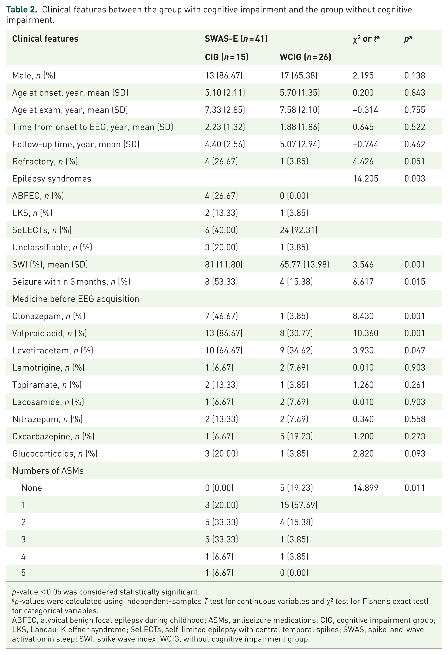
p-value <0.05 was considered statistically significant.
p-values were calculated using independent-samples T test for continuous variables and χ² test (or Fisher’s exact test) for categorical variables.
ABFEC, atypical benign focal epilepsy during childhood; ASMs, antiseizure medications; CIG, cognitive impairment group; LKS, Landau–Kleffner syndrome; SeLECTs, self-limited epilepsy with central temporal spikes; SWAS, spike-and-wave activation in sleep; SWI, spike wave index; WCIG, without cognitive impairment group.
Classification models based on SWI
The model constructed using a single SWI feature showed marked limitations in classification performance. The accuracy of the SVM was 0.732, while that of LightGBM showed a modest improvement to 0.756 (Table 3). The corresponding ROC curves and confusion matrixes for all classification models are presented in Figures 3 and 4.
Evaluation metrics of the model.
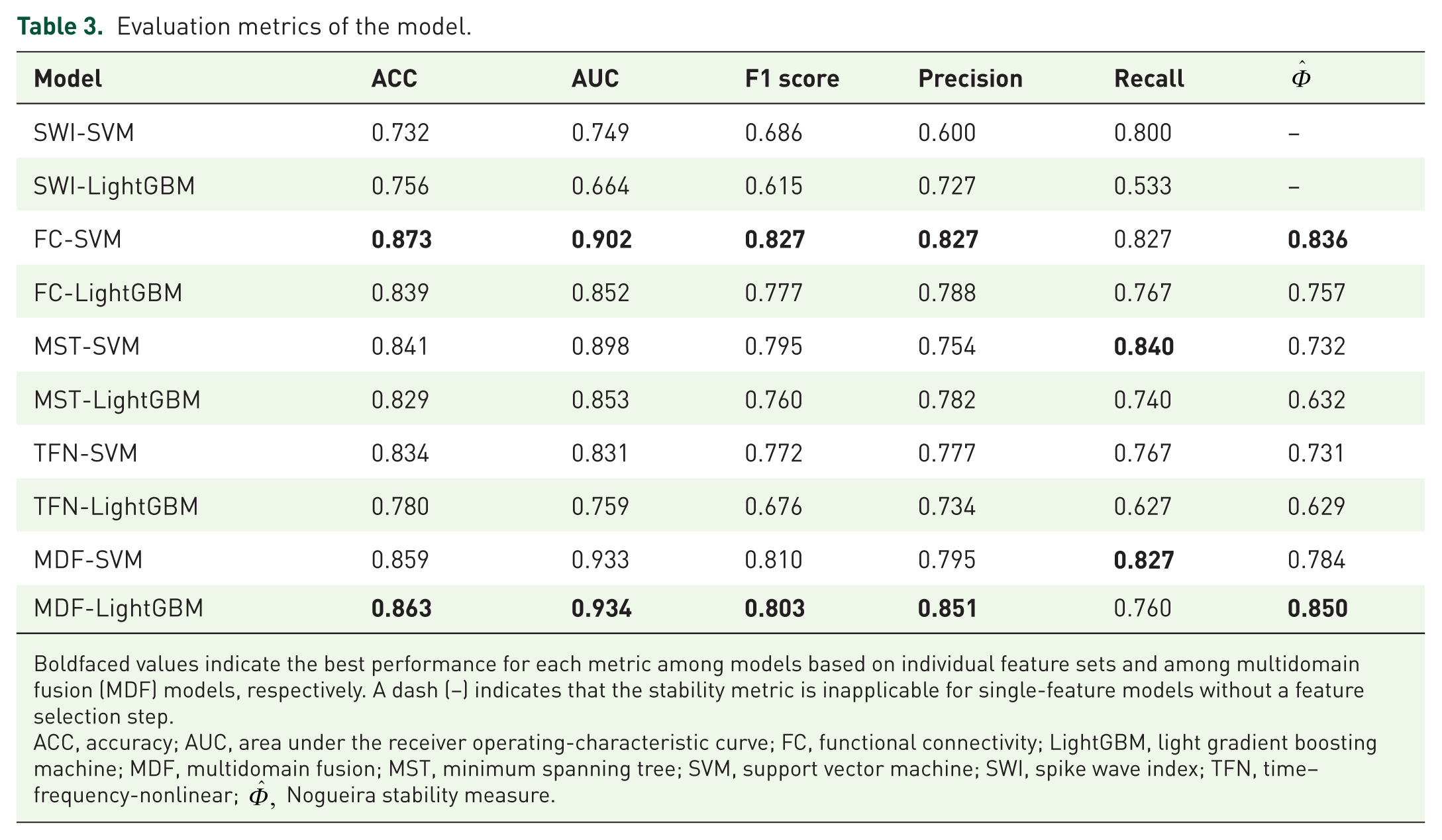
Boldfaced values indicate the best performance for each metric among models based on individual feature sets and among multidomain fusion (MDF) models, respectively. A dash (–) indicates that the stability metric is inapplicable for single-feature models without a feature selection step.
ACC, accuracy; AUC, area under the receiver operating-characteristic curve; FC, functional connectivity; LightGBM, light gradient boosting machine; MDF, multidomain fusion; MST, minimum spanning tree; SVM, support vector machine; SWI, spike wave index; TFN, time–frequency-nonlinear;
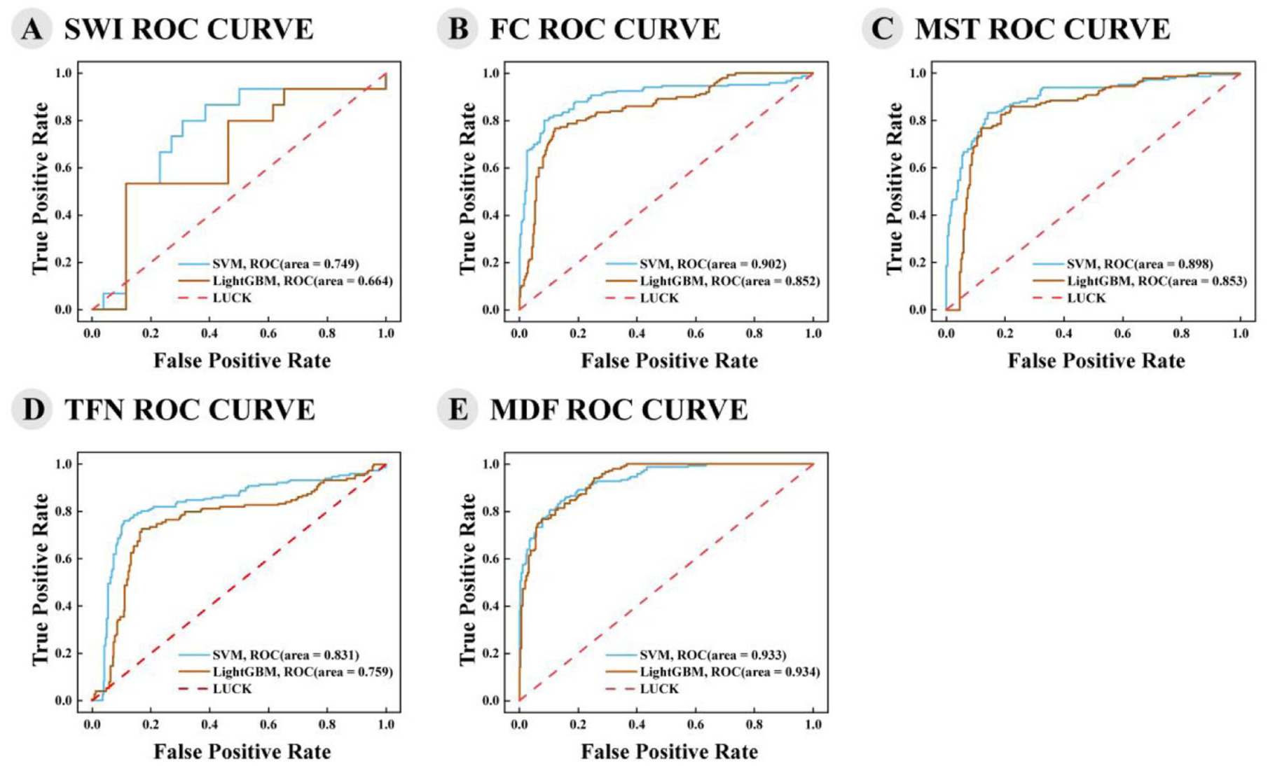
ROC curves of the five feature sets. (a) SWI; (b) FC; (c) MST; (d) TFN; (e) MDF.
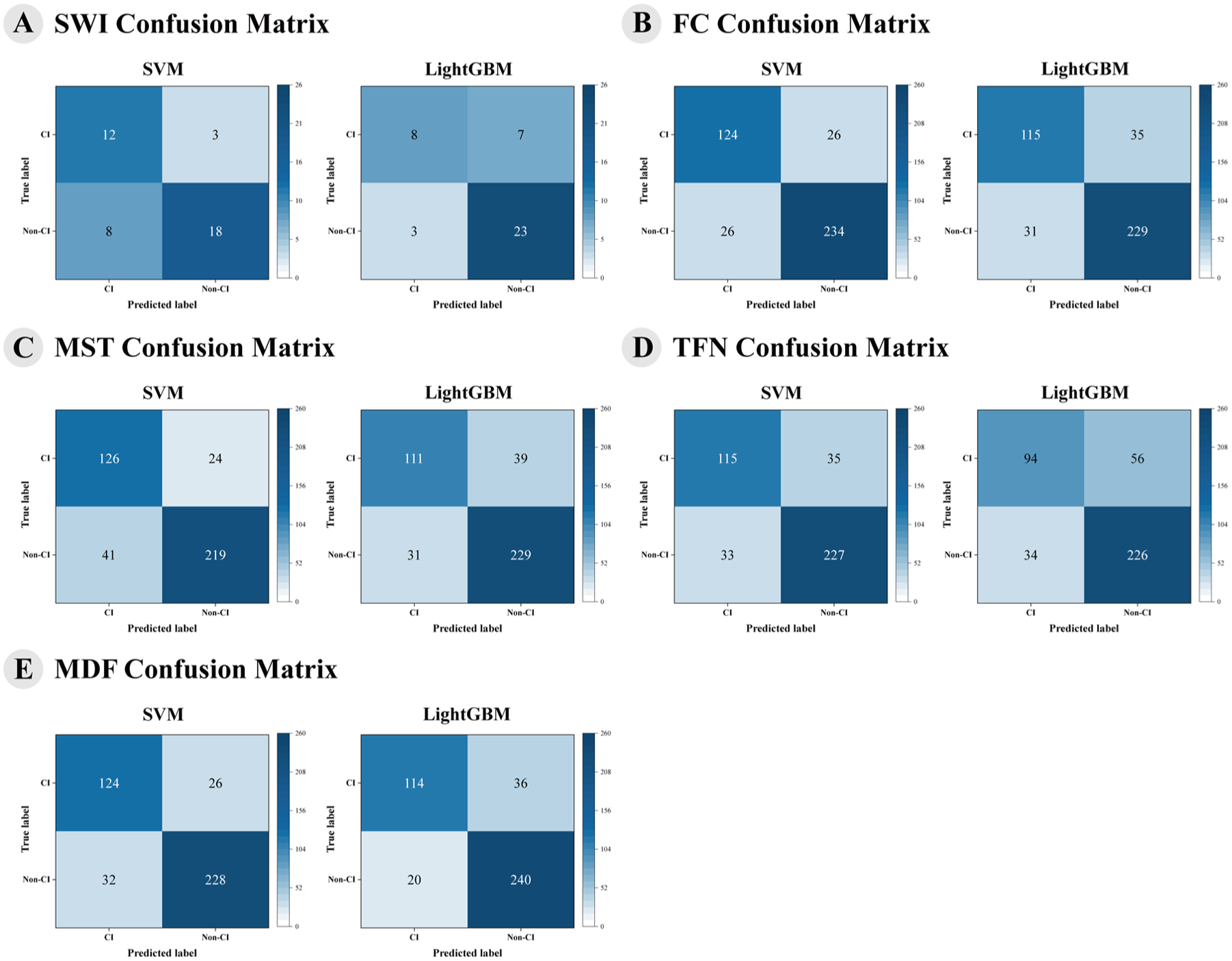
Confusion matrices of the five feature sets. (a) SWI; (b) FC; (c) MST; (d) TFN; (e) MDF.
Classification models based on FC features
Within the FC feature set, the SVM not only outperformed LightGBM across all metrics within this feature set but also achieved the best ACC among all models (Table 3). Both models exhibited high stability
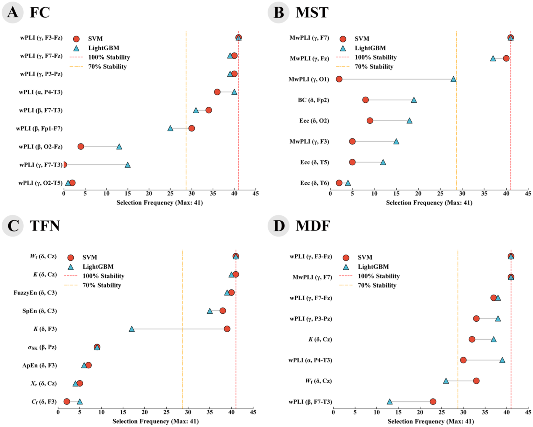
Cross-model stability of highly discriminative features. Selection frequency of EEG features across 41 cross-validation folds. (a) FC; (b) MST; (c) TFN; (d) MDF.
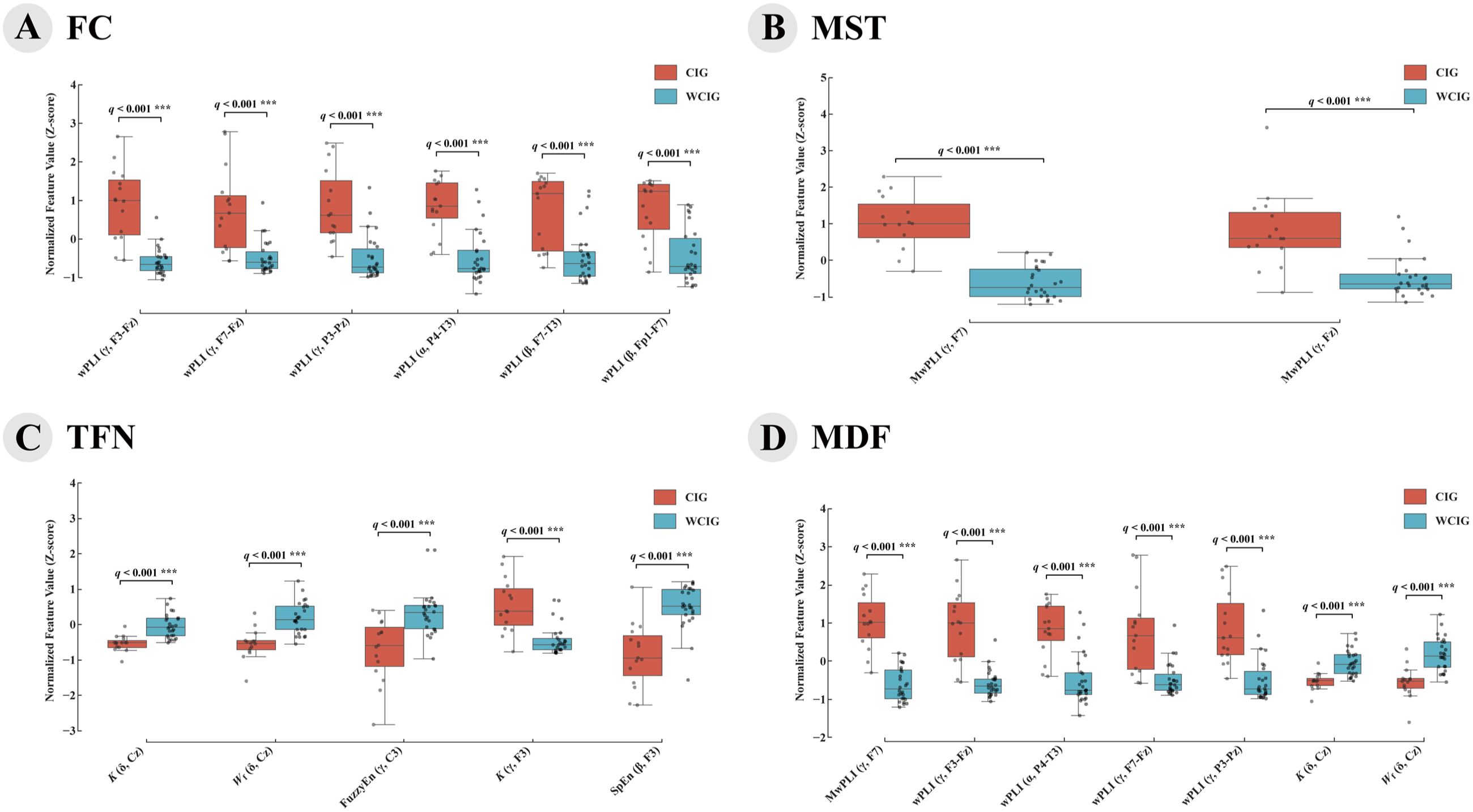
Distribution and statistical comparison of the most stable EEG features across different feature domains. (a) FC; (b) MST; (c) TFN; (d) MDF.
Classification models based on MST features
Within the MST feature set, the SVM model achieved higher accuracy (0.841 vs 0.829) and AUC (0.898 vs 0.853) compared to LightGBM (Table 3). Both models demonstrated relative stability, with the SVM and LightGBM reaching 0.732 and 0.632 (Table 3). Features with a stability greater than 70% (Figure 5(b)) revealed that the nodal connectivity degree (MwPLI) was significantly higher in the CIG than in the WCIG (Figure 6(b)). These stable features were highly localized, concentrating exclusively in the frontal region (F7, Fz) and specifically within the γ frequency band.
Classification models based on TFN features
Within the TFN feature set, the SVM model achieved higher accuracy (0.834 vs 0.780) and AUC (0.831 vs 0.759) compared to LightGBM (Table 3). Both models demonstrated relative stability, with the Nogueira stability measures for the SVM and LightGBM reaching 0.731 and 0.629. Features with a stability greater than 70% (Figure 5(c)) revealed that the CIG exhibited lower entropy (fuzzy entropy and sample entropy), a smaller waveform factor, and lower δ-band kurtosis compared to the WCIG, while demonstrating higher γ-band kurtosis (Figure 6(c)). These stable features were mainly distributed in the central (Cz, C3) and frontal (F3) regions, while spanning the δ, β, and γ frequency bands.
Classification models based on MDF features
Within the MDF feature set, the LightGBM model slightly outperformed the SVM model in both accuracy (0.863 vs 0.859) and AUC (0.934 vs 0.933). Both models exhibited high stability
Discussion
This study developed machine learning prediction models for cognitive impairment in patients with SWAS based on EEG data, achieving high classification accuracy. Although SWI is regarded as the gold standard for diagnosing SWAS, it exhibited limited performance in predicting future cognitive impairment. While SWI can capture the overall epileptic burden and exhibits statistical differences at the group level, its capacity as a predictive biomarker for cognition remains unverified. The substantial overlap in SWI distribution between the two groups renders it insufficient for precise, individual-level cognitive prediction. This limitation remains one of the major barriers to the early identification of cognitive impairment in this disorder. Compared to the SWI-based models, the EEG-based models developed in this study demonstrated better discriminative performance. Specifically, the SVM model based on FC features achieved the highest ACC (0.873), while the MDF models outperformed all single-feature-set models in terms of AUC, exceeding 0.930 (Table 3). The exceptional AUC of the MDF models can be attributed to the synergistic integration of features across multiple dimensions, which provides a more comprehensive electrophysiological profile of the patients. Furthermore, these top-performing models demonstrated robust generalizability, achieving high stability across cross-validation folds. Therefore, these stable EEG models hold the potential to provide an objective basis for early cognitive prediction and precision medication in patients with SWAS.
The predictive model for cognitive impairment proposed in this study demonstrated strong potential for clinical application, particularly for the early screening and intervention support of cognitive impairment in patients with SWAS. First, the model is constructed solely from EEG features and can be easily integrated into existing EEG assessment workflows without additional examination costs. Second, current clinical practice primarily relies on the SWI to guide medication, where patients with a high SWI are often prescribed aggressive treatments. However, SWI acts as a highly sensitive but low-precision indicator, frequently encompassing a significant number of patients who will not eventually develop cognitive impairment. This creates a clinical dilemma between treatment hesitation and overtreatment. The proposed model demonstrates the potential to significantly improve predictive precision over SWI. By providing a more accurate and objective assessment, the model can assist clinicians in making better-informed treatment decisions.
Both FC and MST analyses revealed significantly increased network connectivity during the N3 stage in the CIG. These pronounced increments were predominantly observed in the γ and β bands, with core nodes highly concentrated in the frontal (F3, F7, Fz, Fp1) and parieto-temporal (P3, Pz, P4, T3) regions (Figure 6(a) and (b)). Similarly, Mott et al. reported that patients with ESES exhibited significantly higher coherence during NREM sleep compared with healthy controls, with this enhancement broadly distributed across multiple frequency bands and cortical regions. 25 They suggested that excessive network connectivity might be maladaptive to increased cognitive demands, which may be associated with cognitive and behavioral impairment. However, Mott et al.’s work was limited to comparisons between ESES patients and healthy controls, while we further subdivided SWAS patients according to cognitive status, providing new evidence in support of this hypothesis. Ouyang et al. observed globally increased synchrony during N1 and N2 sleep stages in ESES patients and reported a strong positive correlation between the spike index and global synchrony, 26 though their analysis also lacked subgrouping. In our study, a similar pattern was observed during the N3 stage, where patients with cognitive impairment showed significantly higher SWI values (Table 2), suggesting that enhanced synchrony in this group may be associated with elevated SWI.
TFN analysis revealed significantly lower entropy in the CIG. Additionally, the CIG exhibited an increased γ-band kurtosis, whereas both kurtosis and waveform factor were notably reduced within the δ band (Figure 6(c)). Lower entropy indicates diminished EEG complexity and weaker information processing. 27 In healthy individuals, EEG entropy during N3 is significantly reduced relative to both wakefulness and light sleep, which is a normal physiological phenomenon dominated by high synchrony of slow waves, 28 closely related to synaptic plasticity regulation and memory consolidation.29,30 However, in SWAS patients, epileptic spike waves interfere with or replace these physiological slow waves. Thus, the further decreased entropy observed in the CIG may reflect a more severe pathological hyper-synchronization caused by epileptiform discharges, rather than enhanced normal slow-wave activity. This pathological state may interfere with slow-wave-dependent memory consolidation processes, which are closely associated with cognitive impairment. Additionally, kurtosis is a statistical metric that quantifies the presence of extreme amplitude transients or sharp peaks in a time-series signal, and it is commonly used to identify pathological discharges within epileptic networks.31,32 The significantly elevated kurtosis in the γ band may reflect an increased burden of abnormal discharges within this range. Furthermore, the decreased δ-band kurtosis and waveform factor might suggest a weakening or flattening of physiological slow-wave features, possibly reflecting a disruption of slow-wave homeostasis. Collectively, these abnormal alterations in EEG may be closely associated with the underlying cognitive impairment in SWAS patients.
Notably, despite the substantial physiological differences among the three feature sets, the highly stable features consistently converged on frontoparietal regions and specific frequency bands (β, γ, and δ), suggesting that these specific cortical networks and interrelated brain rhythms may be closely related to cognitive impairment in patients with SWAS.
The simultaneous alterations observed in both fast activity (β and γ) and slow-wave (δ) may signify a global disruption of brain rhythm coordination in SWAS, which may be closely associated with cognitive impairment. Valderrama et al. conducted a macroscopic EEG study and found that γ oscillations appeared simultaneously in the “UP” and “DOWN” phases of slow waves, tightly coupled with the slow-wave phase. 33 This coupling may be involved in memory consolidation and offline information processing during sleep. Furthermore, previous studies have also demonstrated that a reduction in the slope of slow waves has been observed in patients with ESES, reflecting a disruption of synaptic homeostasis and alterations in slow-wave structure.10,34 In our study, these concurrent alterations in fast and slow-wave activities may represent a distinct neurophysiological signature of cognitive impairment in patients with SWAS.
The highly discriminative features frequently appeared in the frontotemporal (F3, F7, Fz, Fp1) and parieto-temporal (P3, Pz, P4, T3) regions, likely due to the close association between the corresponding brain regions and SWAS. First, SWAS is often characterized by frontal lobe dominance in EEG recordings using the 10-20 system, although this could be an artifact of VC effects. 35 Second, frontotemporal regions are highly involved in higher cognitive functions such as language and executive functions,36,37 which are frequently impaired in SWAS patients. 38 Furthermore, the concurrent involvement of parietal regions strongly implicates the frontoparietal network (FPN). The FPN plays a crucial role in working memory capacity and complex cognitive control. 39 These associations may explain the frequent appearance of features related to these specific cortical regions in the analysis. Moreover, Valderrama et al. also found that two phase coupling modes between slow waves and γ waves predominantly occur in the frontotemporal regions, 33 which aligns with the frequent appearance of γ-band features discussed earlier.
This study has certain limitations that may affect the generalizability and reliability of the results. First, the potential confounding effect of medication exposure cannot be entirely eliminated. Although we incorporated medications with significant differences between groups as covariates to mitigate this issue, it remains difficult to guarantee that the selected EEG features are completely free from the influence of medications in a retrospective study. Therefore, future prospective studies are warranted to better address this limitation and validate these biomarkers. Second, the data were derived from a single-center and are limited by a small sample size, lacking multicenter and multiregion data, which restricts the applicability of the findings to a broader population. Third, the study only included N3 sleep EEG data, which may not be applicable to patients with sleep disorders or those who cannot accurately identify sleep cycles. Moreover, this study did not cover the full spectrum of EE-SWAS etiologies, which will need to be further addressed in future studies.
Conclusion
This study developed EEG-based machine learning models that could help predict future cognitive outcomes in SWAS patients. EEG features have the potential to serve as valuable biomarkers for early identification of cognitive impairment in SWAS patients and may assist in diagnosis and treatment in future clinical settings. However, given the preliminary nature of these findings and current methodological limitations, further clinical verification is warranted.
Supplemental Material
sj-docx-1-tan-10.1177_17562864261453784 – Supplemental material for Prediction of cognitive impairment in epilepsy with spike-and-wave activation in sleep based on EEG
Supplemental material, sj-docx-1-tan-10.1177_17562864261453784 for Prediction of cognitive impairment in epilepsy with spike-and-wave activation in sleep based on EEG by Rui Han, Jialing Li, Cuifang Liang, Jun Ma, Jie Luo and Bingwei Peng in Therapeutic Advances in Neurological Disorders
Footnotes
Appendix A
Nonlinear features and interpretation.
| Feature | Symbol | Definition | Interpretation |
|---|---|---|---|
| Power Spectral Entropy | H ps | Measures the flatness or randomness of the power spectrum. | |
| Energy Entropy | H en | Quantifies distribution uniformity of energy in sub-bands. | |
| Approximate Entropy | ApEn | Measures regularity and complexity of time series. | |
| Sample Entropy | SampEn | Improved estimate of complexity, less biased than ApEn. | |
| Fuzzy Entropy | FuzzyEn | Complexity measure using fuzzy membership function, robust to noise. | |
| Permutation Entropy | PE | Quantifies time series complexity based on ordinal patterns. | |
| Envelope Entropy | H env | Reflects randomness of the signal envelope distribution. |
K: number of frequency bins; M: number of sub-bands (or envelope bins); N: number of samples; m: embedding dimension in ApEn, SampEn, FuzzyEn, permutation order in PE; r: similarity tolerance in ApEn, SampEn, scale parameter in FuzzyEn; pk: normalized spectral power probability; qi: normalized energy probability in sub-band i; ei: normalized envelope amplitude probability; Um: probability of matched patterns of length m (without self-match); µm: average fuzzy similarity of m-dimensional patterns;
Acknowledgements
The authors thank all data collection personnel for their invaluable contributions to this study.
Declarations
Availability of data and materials
Supplemental material
Supplemental material for this article is available online.
References
Supplementary Material
Please find the following supplemental material available below.
For Open Access articles published under a Creative Commons License, all supplemental material carries the same license as the article it is associated with.
For non-Open Access articles published, all supplemental material carries a non-exclusive license, and permission requests for re-use of supplemental material or any part of supplemental material shall be sent directly to the copyright owner as specified in the copyright notice associated with the article.