Towards the prediction of flame transfer functions: Evaluation of a hybrid LES-CAA with compressible LES

Abstract

The prediction of flame transfer functions, particularly in practically relevant systems, remains challenging and computationally demanding. Numerical approaches are a valuable addition to experimental acoustic characterizations of industrial configurations. Conventionally, fully compressible numerical simulations are used that naturally include acoustic fluctuations in their computations, but can be computationally expensive depending on the configuration. Therefore, a convenient approach to use tailored numerics for the underlying physics is considered in this work. In this work, this is realized by applying a runtime-coupled method of computational fluid dynamics and computational aeroacoustics to a single-sector aero-engine combustor. This hybrid computational fluid dynamics and computational aeroacoustics method captures fluid flow behavior and combustion dynamics in a low-Mach computational fluid dynamics domain while allowing for acoustic perturbations in the computational aeroacoustics. Runtime exchange of hydrodynamic and acoustic quantities between the two solvers allows for a bidirectional coupling and, by extension, a complete description of the combustion system. In this work, the hybrid computational fluid dynamics and computational aeroacoustics is applied in a high-fidelity large eddy simulation configuration. The flame transfer function is evaluated for both compressible and hybrid simulations. The results for both numerical approaches are validated with each other and compared to the experimentally obtained flame transfer function. Finally, the computational effort for the numerical approaches is considered. This article presents the first application of a high-fidelity computational fluid dynamics framework using large eddy simulation with bidirectional coupling with the acoustic solver to an industry-relevant configuration. The aim is to provide a roadmap towards investigating thermoacoustic instabilities in a real gas turbine engine at reduced computational costs.

Keywords

Flame transfer function large eddy simulations hybrid large eddy simulation and computational aeroacoustics compressible large eddy simulation thermoacoustic instabilities gas turbine combustion

Introduction

Global initiatives tackling pollutant emissions in aviation have long started to turn towards lean-burn combustion systems that promise to produce lower ${NO}_{x}$ levels and particulate emissions.^1,2 While advantageous for mitigating global warming, the design of lean-burn systems can be challenging since mixing and heat-release-rate fluctuations possibly lead to thermoacoustic oscillations in the combustion chamber.^3,4 The interplay of these oscillations with the acoustic modes of the combustor geometry potentially leads to thermoacoustic instabilities that compromise engine operation.

To acoustically characterize an aero-engine system, experimental analyses are employed to novel combustors and fuel injectors at different stages of the development process. One reason for these acoustic investigations is to further improve the understanding of the response of the given combustion system to pressure perturbations reaching the combustor due to fluctuations from other stages of the gas turbine system. Specific test benches incorporate these fluctuations and use acoustic measurements for the analysis, such as the test bench considered in this work.

To support the understanding, numerical approaches are often applied to provide additional insight and low turnaround times. From a numerical standpoint, compressible computational fluid dynamics (CFD) simulations are the current state-of-the-art approaches to investigate the thermoacoustic behavior in industrial applications.^5–8 These simulations can resolve combustion and acoustic dynamics in a directly coupled manner. However, accounting for all physical processes in one fluid flow solver can be computationally expensive: While the determinant convective scale in the flow and the combustion domain is in the order of the fluid flow velocity, acoustic waves propagate with the speed of sound. Additionally, the spatial scales that have to be considered vary broadly from small cells to capture the structure of the flame and the chemistry in the combustion chamber, to long wavelengths present in low-frequency combustion instabilities in the engine. For the compressible CFD simulation, this corresponds to small-scale cells for the resolution of the combustion dynamics in addition to relatively smaller time steps to capture the acoustic waves propagating faster than the fluid flow convection.

One possible approach to mitigate this high computational demand is to separate the convective and acoustic domain into dedicated solvers.^7,9 This can be realized using two-step approaches that usually first conduct a fluid flow simulation to obtain mean fluid flow fields to then use them in successive computational aeroacoustics (CAA) simulations. Such approaches have been widely used in the literature for non-reacting conditions¹⁰ or in the context of combustion noise.^11–13 A further possibility is to connect CFD simulations with subsequent system identification to obtain acoustic transfer matrices^8,14,15 or flame transfer functions (FTFs).^5,16

This work is the latest continuation of studies that worked on developing and evaluating a runtime-coupled hybrid computational fluid dynamics and computational aeroacoustics (CFD-CAA) approach first implemented to describe combustion noise phenomena.¹⁷ The approach uses the acoustic perturbation equations (APEs),^18–20 adapted for low-Mach flow fields and including a source term to include the influence from combustion. After having expanded this method to a functioning, bidirectional approach able to capture self-excited thermoacoustic instabilities,²¹ the runtime-coupled, hybrid CFD-CAA method was applied to a realistic combustor configuration.²² The test rig investigated herein has been analyzed by the authors for non-reacting conditions using scale-adaptive simulations (SASs) and CAA simulations,²³ for reacting conditions using hybrid scale-adaptive simulation and computational aeroacoustics (SAS-CAA),²² and for reacting conditions using compressible large eddy simulation (LES).^24,25

In the present study, the hybrid CFD-CAA method is applied to a realistic gas turbine combustor configuration, using LES on the fluid dynamics side for the first time, and comparing the obtained results to compressible LES. Previously, hybrid SAS-CAA computations were conducted, which aimed for general model validation but faced challenges reproducing experimental reference data due to substantial geometrical simplifications. This article employs a more sophisticated geometrical representation of the Scaled Acoustic Rig for Low Emission Technology (SCARLET) configuration. Finally, the operating condition used in this work has been investigated using compressible LES,²⁵ generating extensive numerical data that provides a valuable possibility to benchmark the novel method, and to comprehensively analyze the results.

This article is structured as follows: First, the numerical framework used for the acoustic characterization will be introduced, with a special emphasis on the runtime-coupling between LES and CAA. Then, the investigated test rig will be introduced, first in terms of the experimental configuration, and finally in terms of the computational setup for CFD and CAA. Here, spatial and temporal discretization as well as boundary conditions will be described. The results section of this work will first provide an insight into the flow dynamics in the combustion chamber, comparing the numerical approaches, and then focus on the thermoacoustic behavior. The FTF as main point for comparison will be evaluated using SAS and LES, and the results will be discussed both in comparison with the experiment, and in terms of the computational effort.

Numerical framework

In this work, two main numerical approaches are used to compare the computed FTF of an industry-relevant combustion configuration to the experimentally measured one. This section will introduce the solvers for CFD and CAA, as well as the coupling methodology used for the hybrid CFD-CAA approach.

CFD solver

The Rolls-Royce in-house CFD solver PRECISE-UNS²⁶ is used to solve the Navier-Stokes equations. It is developed and maintained specifically for the simulation of reacting flows in the context of aero-engine combustion. It allows for compressible simulations via a pressure-correction method with an extension to compressible flows.²⁷ Most commonly and also in the context of the hybrid large eddy simulation and computational aeroacoustics (LES-CAA) method, it is employed in a low-Mach formulation, which allows for density variation due to heat release. The density $ϱ$ is evaluated using the ideal gas law, considering the static pressure $p_{static}$ , the specific gas constant $R_{s}$ , and the temperature $T$ :

ϱ = \frac{p_{static}}{R_{s} T}

(1)

For LES computations, turbulence is treated using the

σ

subgrid viscosity model with a global model constant of

C_{σ} = 1.35

.²⁸ For additional reference simulations, a SAS approach is used.²⁹

For all cases in the present work, spatial discretization of the diffusive fluxes, as well as the pressure-correction equation, use a second-order central scheme, while convective fluxes are discretized using a second-order total variation diminishing scheme.³⁰ The equations are advanced in time using a second-order accurate backward-differences scheme.

CAA solver

The hybrid LES-CAA approach couples a low-Mach flow solver such as PRECISE-UNS to the dedicated acoustics solver of the open-source framework Nektar++.³¹ This framework uses spectral/ $h p$ element methods, which are used in a discontinuous Galerkin formulation for high-resolution spatial discretization. Temporal discretization is realized using a low-dispersion, fourth-order Runge-Kutta scheme. For the description of the propagation of acoustic waves, the Nektar++ framework provides the AcousticSolver, which implements versions 1 and 4 of the Acoustic Perturbation Equations.¹⁸ The APEs describe the spatial and temporal evolution of linearized acoustic perturbation quantities such as pressure $p^{a}$ and velocity $u^{a}$ around a mean flow field defined by the mean flow quantities density $\bar{ϱ}$ , fluid flow velocity $\bar{u}$ , and speed of sound $\bar{c^{2}}$ . The definition of the APEs follows equation (2):

\begin{aligned} \frac{\partial p^{a}}{\partial t} + \bar{c^{2}} \nabla \cdot (\bar{ϱ} u^{a} + \bar{u} \frac{p^{a}}{\bar{c^{2}}}) & = q_{c}^{'} + q_{e}^{'} + q_{c & e}^{'} \\ \frac{\partial u^{a}}{\partial t} + \nabla (\bar{u} \cdot u^{a}) + \nabla \frac{p^{a}}{\bar{ϱ}} & = q_{m}^{'} \end{aligned}

(2)

where the superscripts

\bar{(-)}

(-)^{'}

, and

(-)^{a}

denote mean, fluctuating, and acoustic quantities, respectively. The APEs can include instantaneous influences of flow and combustion dynamics using right-hand side source terms

q_{i}^{'}

for pressure and

q_{m}^{'}

for velocity. The right-hand side source terms arise from the linearization of the mass (

q_{c}^{'}

), energy (

q_{e}^{'}

), and momentum (

q_{m}^{'}

) conservation, and by coupling the mass and energy equations to obtain a two-equation system for the dependent variables acoustic pressure and acoustic velocity (

q_{c & e}^{'}

).²⁰

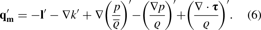
The source terms for low-Mach (i.e., without acoustic components) and single-species flow can be simplified to^18,20,32:

q_{c}^{'} = - \bar{c^{2}} \nabla \cdot {(u^{'} ϱ^{'})}^{'}

(3)

q_{e}^{'} = - \bar{c^{2}} \frac{\partial ϱ}{\partial t}

(4)

q_{c & e}^{'} = - \bar{c^{2}} \nabla \cdot {(\bar{u} ϱ^{'})}^{'}

(5)

q_{m}^{'} = - l^{'} - \nabla k^{'} + \nabla {(\frac{p}{\bar{ϱ}})}^{'} - {(\frac{\nabla p}{ϱ})}^{'} + {(\frac{\nabla \cdot τ}{ϱ})}^{'}

(6)

For nonreactive and isothermal flows, the momentum source

q_{m}^{'}

with the Lamb vector

l

is dominating the acoustic source terms. Geiser et al.²⁰ expanded on the importance of the energy source term for reacting flow simulations.

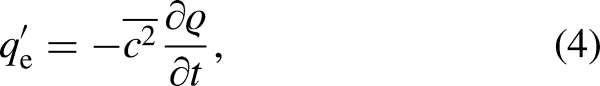
For the considered system, the pressure equation source terms from equations (3) to (5) are displayed in Figure 1, using a logarithmic scale. From the direct comparison, it is evident that the energy source term $q_{e}^{'}$ is predominant. Hence, other acoustic sources are excluded from the simulations in this work.

Figure 1.

Time-averaged values of the pressure source terms in the combustion chamber, evaluated from large eddy simulation (LES) computation. Note the logarithmic scale. (a) $\log (| q_{e}^{'} |)$ ; (b) $\log (| q_{c & e}^{'} |)$ ; and (c) $\log (| q_{c}^{'} |)$ .

LES-CAA coupling

In thermoacoustic systems, different physical phenomena can merit a different treatment in numerical simulations. In Table 1, some scale information on combustion and convection on the one side, and acoustics on the other side are displayed. The differences in both length and time scales described there motivate the use of a hybrid approach that separates the respective physics into distinct numerical methods. This section will describe the reasoning behind the bidirectional coupling of CFD and CAA solvers, and the coupling methodology in more detail.

The coupling between PRECISE-UNS and the AcousticSolver was first introduced for combustion noise computations, where the sound emitted from a flame can be assessed.¹⁷ The external coupling library CWIPI (coupling with interpolation parallel interface), developed at ONERA,³³ was included that can exchange information from different code bases and different spatial and temporal discretizations. For combustion noise, fluid flow information is transferred to the acoustic domain, which includes mean fluid flow quantities and necessary source terms. LES of combustion noise investigations were conducted using this so-called forward-coupling to great success.¹⁷ The general architecture of the coupling at that time already allowed for acoustic quantities to be sent back to the CFD, though their implementation in the workings of the CFD flow solver was not yet realized.

Table 1.

Limiting scales.

CFD	CAA
Limiting length scales
Turbulence & flame	Acoustic wave length
$O (10^{- 3} m)$	$O$ (m)
Limiting time scales
From convection velocity	From speed of sound
$O (10^{- 5} s)$	$O (10^{- 6} s)$

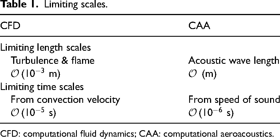
CFD: computational fluid dynamics; CAA: computational aeroacoustics.

Later, a backward coupling was implemented²¹ to equally apply the bidirectionally coupled CFD-CAA method to investigate thermoacoustic instabilities, where acoustic fluctuations lead to changes in fluid flow quantities. The functionality of the bidirectional coupling was first validated using a generic, two-dimensional test case exhibiting self-excited oscillations.²¹ Finally, the method was successfully applied to a complex, three-dimensional configuration, using low-resource SASs to accomplish a general validation for a combustion chamber investigation.²²

Figure 2 depicts the coupling between CFD and CAA solvers, the quantities that are exchanged, and the coupling intervals. The acoustic pressure fluctuations are transported to the CFD and used within the density computation to account for density changes associated with acoustics to realize a backward coupling from acoustics to fluid flow. The influence on the density 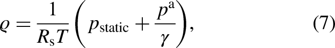$ϱ$ is described by equation (7):

ϱ = \frac{1}{R_{s} T} (p_{static} + \frac{p^{a}}{γ})

(7)

where

γ

is the isentropic exponent.

Figure 2.

Schematic diagram of the exchange of coupling quantities between CFD and CAA simulations. CFD: computational fluid dynamics; CAA: computational aeroacoustics.²¹

Since the temporal change in density is introduced as a source term into the low-Mach formulation of the pressure–velocity coupling, this change in density results in a corresponding change in both pressure and velocity. Hence, this introduces the influence of acoustic fluctuations on the low-Mach CFD simulation.

Configuration and setup

Experimental setup and prior investigations

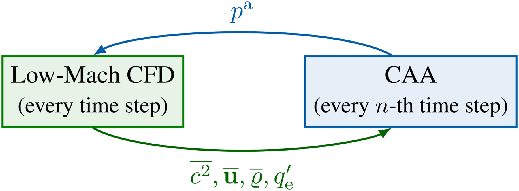
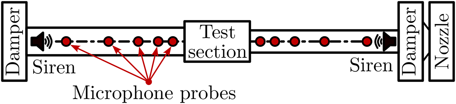
The considered configuration is a combustion chamber designed for the experimental acoustic characterization of any given realistic aero-engine fuel injector. The SCARLET is the Rolls-Royce thermoacoustic rig, operated at DLR Cologne.^34,35 It provides two methods to assess the thermoacoustic response of the system to acoustic excitation: On the one hand, acoustic measurement via a multi-microphone method,^36,37 and on the other hand, optical measurement via the OH* chemiluminescence using the available optical access. A schematic diagram of the test rig is depicted in Figure 3, including sirens and dampers ensuring defined acoustic boundary conditions, and the acoustic measurement sections upstream and downstream of the test section. The test section—comprising injector, outer annulus, and combustion chamber—also includes an optical access window to the combustion chamber to measure OH* chemiluminescence (see Figure 4).

Figure 3.

Schematic diagram of the Scaled Acoustic Rig for Low Emission Technology (SCARLET) measurement setup, including measurement section and sirens and dampers on both sides.

Figure 4.

Schematic diagram of the Scaled Acoustic Rig for Low Emission Technology (SCARLET) test section, including the optical access to measure ${OH}^{*}$ chemiluminescence and the reference position.

Both methods result in the flame transfer function (FTF). However, they are based on different assumptions during the evaluation. The multi-microphone method treats the test section as an acoustic two-port. Using matrix relations for the transfer matrices of the configuration with and without combustion, the flame transfer matrix (FTM) can be obtained. The FTF is then evaluated by means of one element of the four-element FTM. The optical measurements allow for a direct evaluation of the heat-release rate in the combustion chamber, which, in relation to the acoustic velocity signal at the reference position of the configuration, yields the FTF. Since the comparison to the experimentally obtained FTF is not the main scope of this work, the measurement techniques will not be described in more detail. However, for the multi-microphone method, it was concluded in other works that its application to this configuration in a numerical context is prone to errors because of underlying assumptions.^25,22 A more advanced post-processing with better comparability between numeric approaches and the experimental FTF is currently being investigated at the Institute for Simulation of reactive Thermo-Fluid Systems (STFS) of TU Darmstadt.

For the optically evaluated FTF, the comparison to the heat-release-rate-based FTF of a compressible LES has provided satisfactory results for a system of such complexity.²⁵

Evaluating the FTF from numerical simulations

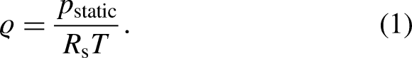
Thermoacoustic characterization of a combustion system can be realized using the FTF. It relates combustion and acoustic fluctuations, and is generally defined as follows:

FTF (ω) = \frac{{\dot{Q}}^{'} (ω) / \bar{\dot{Q}}}{u_{ref}^{'} (ω) / \bar{u}}

(8)

Here,

{\dot{Q}}^{'} (ω) / \bar{\dot{Q}}

are the normalized global heat release fluctuations and

u_{ref}^{'} (ω) / \bar{u}

are the normalized acoustic velocity fluctuations at a reference position upstream of the flame. The reference position for both experiments and the numerical simulations is located at the very end of the upstream duct, that is, upstream of both injector and flame, cf. Figure 4. In the experimental SCARLET configuration, a small window for endoscopic imaging of the flame behavior inside the combustion chamber is available. Optical measurement sections record the chemiluminescence of the OH* which is assumed to correspond to the heat-release rate³⁸

\frac{{\dot{Q}}^{'} (ω)}{\bar{\dot{Q}}} \propto \frac{{OH}^{*'}}{\bar{OH *}}

(9)

However, since this measurement is of significantly higher maintenance effort, this data is only available for a limited number of cases. More detail on the computation of the FTF from

OH *

measurements for the SCARLET setup is published in literature.^38,25 Since, in a numerical context, point information of all necessary quantities in the entire computational domain is available, the FTF can be obtained using the response of the flame to acoustic excitation. This is realized in terms of the global heat-release rate

\dot{Q}

, which is the integrated local heat-release rate

\dot{q}

over the simulation domain

Ω

\dot{Q} = \int_{Ω} \dot{q} (x_{i}) d Ω

(10)

For the computation of the FTF, pressure and velocity fluctuations (

p^{'}

and

u^{'}

, respectively) are recorded at the microphone positions in the upstream duct, cf. Figure 3. The velocity fluctuations at the reference position are obtained by decomposing the plane wave in the upstream duct into upstream- and downstream-traveling components, and evaluating them at the reference position. The computation of the FTF follows closely the approaches taken in previous work,^25,22 and will not be reiterated here.

In the evaluation procedure, mean flow field quantities are included, namely the mean hydrodynamic density $\bar{ϱ}$ , the mean speed of sound $\bar{c}$ , and the mean upstream convection velocity $\bar{u}$ are necessary. They are obtained by a precursor low-Mach CFD simulation.

Figure 5 display FTFs obtained by the optical measurement approach, comparing the FTF as postprocessed from SAS and LES. The compressible SAS is conducted on a coarse, tetrahedral mesh with around 1.5 million control volumes (cf. Reinhardt et al.²²), while the LES is applied to a significantly higher resolved numerical representation comprising around 11 million control volumes. As will be the case for results later in this work, the FTF is displayed in terms of its absolute gain value and the corresponding phase angle. The phase angle is wrapped to only allow for values between $[- π, 2 π]$ , which allows for a good visual comparison between both the phase angle values and the slope between two neighboring values. In all figures displaying FTF, the experimental values are provided as additional reference, mainly for the compressible CFD simulations. The gain values of the compressible simulations display significant differences between the two cases, with mixed agreement with the experiment. As other investigations have shown, the gain value comparison of the compressible CFD simulations to the experiment is also to be considered with caution.²⁵ For this work, the compressible CFD results for the gain values are therefore chosen as reference for the hybrid approach, without strongly taking into account the agreement with the experimental data.

Figure 5.

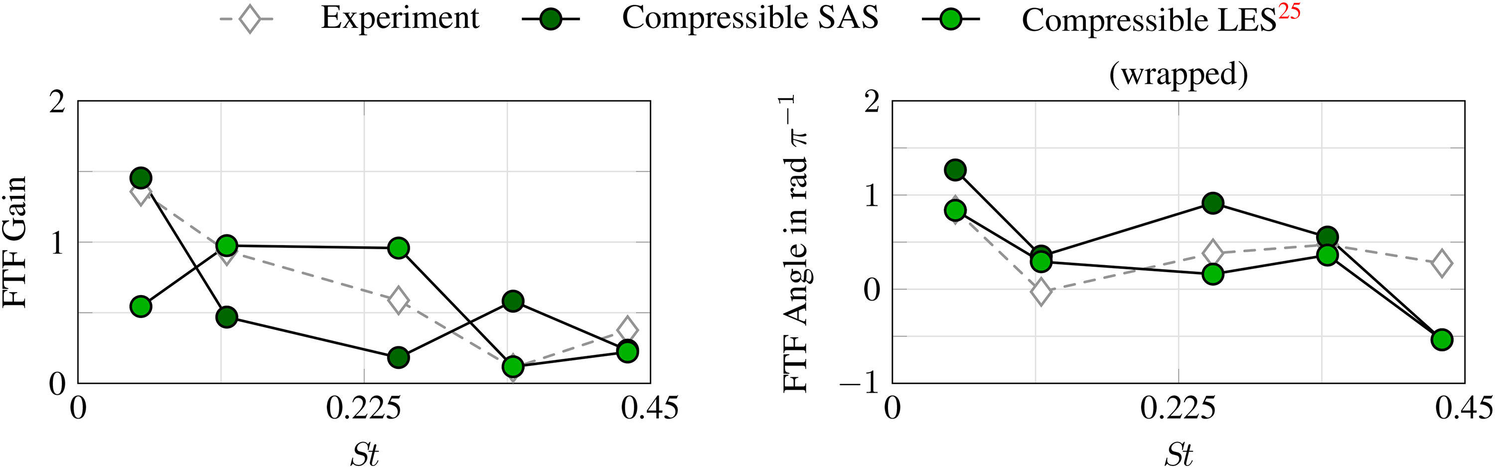
Flame transfer function from compressible computations, for (dark green circles) SAS and (light green circles) LES,²⁵ compared to (gray diamonds) experiment. SAS: scale-adaptive simulation; LES: large eddy simulation.

Figure 6.

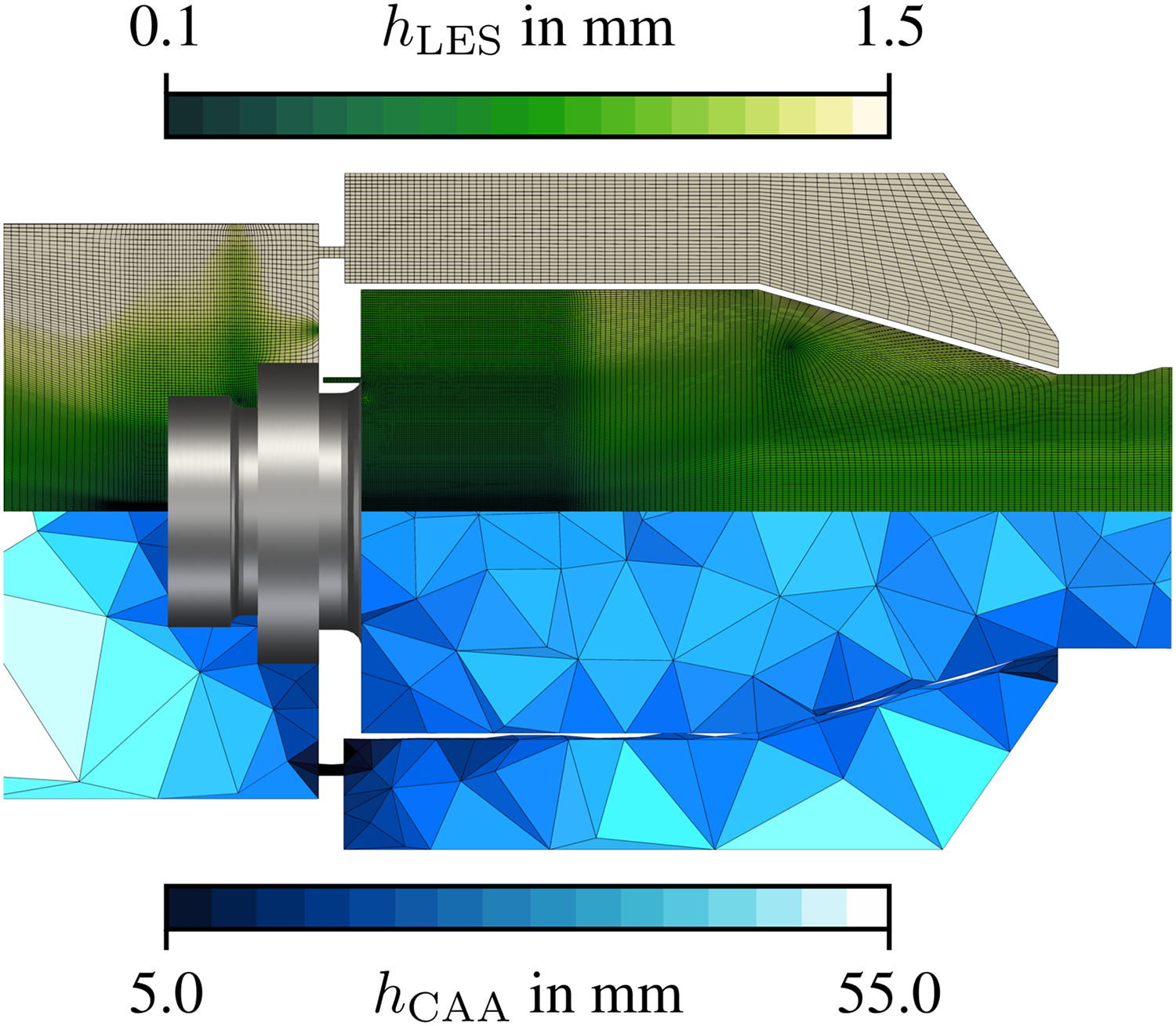
Computational grids and mesh sizes for LES (green) and CAA (blue). LES: large eddy simulation; CAA: computational aeroacoustics.

The phase angles are considered better comparable between experiment and numerical simulations. They provide a sense of the convective behavior and time lags of the thermoacoustic system, with the phase angle curve’s slope corresponding to the phase shift between the input ( $u^{'}$ ) and output signals ( ${\dot{Q}}^{'}$ ). For the lowest frequency points, the slope of the compressible SAS’ phase values is almost parallel to the experimental reference, while the phase angle slope is flatter in the case of compressible LES. Both numerical approaches end at the same phase shift for the highest frequency. Generally, the phase shift between both compressible SAS and LES, and the experimental data are of mostly low value, with a maximum phase shift lower than $π$ for the third and last frequencies.

Boundary conditions

The advantages of the hybrid CFD-CAA method can be primarily seen in the comparative ease of handling the boundary conditions and the separation of scales in the spatial and temporal domains. This section will introduce the boundary conditions used in the two numerical approaches.

Inlet boundary

Both low-Mach and compressible CFD simulations specify a constant mass flow at the inlet boundary. In the compressible CFD, the inlet is specified as NSCBC (Navier-Stokes characteristic boundary condition)³⁹ with plane wave masking.¹⁴ Any acoustic excitation is specified by means of the amplitude of the incoming acoustic wave. In the hybrid CFD-CAA method, the acoustic excitation is specified as a pressure time signal in the CAA solver.

Outlet boundary

Static pressure is defined at the outlet boundary for the low-Mach CFD simulation. In the case of CFD-CAA coupling, the outlet pressure is allowed to change subject to the respective acoustic perturbations; it is set to $p_{static} = 0 Pa + p^{a}$ . In the CAA solver, the acoustic non-reflectivity is addressed using the Riemann invariant boundary conditions. In the compressible CFD, the outlet boundary is set to an absolute pressure value corresponding to the experiment. For acoustic simulations, it is also specified as NSCBC³⁹ with plane wave masking.¹⁴ This boundary exhibits almost no acoustic reflections when affected by outgoing plane waves. Chosing non-reflecting outlet boundary conditions allows for a simple alternative to specifying end-reflection values, and is considered true to the experiment, where low reflectivity is ensured by operating acoustic dampers.

Effusion boundaries

Effusion boundaries in PRECISE-UNS are used to transport mass, momentum, and energy from one boundary patch to another, mimicking the actual transport of fluid through orifices. Most importantly, this is used for the effusion liner, which contains thousands of small effusion holes, which, if resolved, would lead to an excessive amount of necessary computational resources. The effusion liner boundary patch is defined by a total mass of ${\dot{m}}_{liner} = 0.3 {\dot{m}}_{inlet}$ and a defined angle into the combustion chamber. Additionally, effusion boundaries are specified for small passages that, in the experimental configuration, lead from the upstream duct behind the heat shield.

Combustion and spray

The flamelet generated manifold (FGM) approach⁴⁰ describes the chemical kinetics. The flamelets are computed with CHEM1D,⁴¹ a one-dimensional flame solver. The progress variable for the composition, 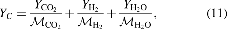$Y_{C}$ is defined as follows:

Y_{C} = \frac{Y_{C O_{2}}}{M_{C O_{2}}} + \frac{Y_{H_{2}}}{M_{H_{2}}} + \frac{Y_{H_{2} O}}{M_{H_{2} O}}

(11)

where

Y_{i}

and

M_{i}

are the mass fraction and molar mass of species

i

, respectively. The fuel is kerosene (Jet-A1) and it is characterized by the dodecane mechanism which contains 57 species and 273 reactions.⁴²

The liquid fuel is injected at two discrete ring-shaped regions at the end of the swirl passages near the (pilot) pressure-swirl and the (main) airblast atomizers. The spray is modeled as Lagrangian parcels with a prescribed Sauter mean diameter (SMD), initial velocity, temperature, and fuel mass flow rate. At each injection time step, the diameters of the parcels are sampled following a Rosin-Rammler distribution with prescribed statistical properties. At the walls, the parcels are assumed to reflect, respecting the conservation of momentum. A steady-state evaporation model for the droplets is used.⁴³ The spray parameters chosen for this work are based on Rolls-Royce best practice.

Acoustic excitation

The acoustic forcing in all numerical simulations is realized in terms of a time signal of pressure and velocity perturbations. It is introduced either at the upstream or the downstream end of the (compressible CFD or CAA) domain, representing the signal of the sirens used in the experiment. The chosen time signal $s (t)$ is a multi-sine signal of $N_{freq} = 5$ frequencies, realized by superposition with defined amplitudes $A_{k}$ and Newman’s phases $φ_{k}$ ,⁴⁴ that provide maximum spectral content with the least instantaneous amplitude and a low crest factor,

s (t) = \sum_{k = 1}^{N_{freq}} A_{k} \sin (ω_{k} t + \underset{φ_{k}}{\underset{⏟}{\frac{π (k - 1)^{2}}{N_{freq}}}})

(12)

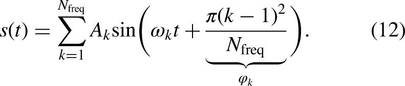
The signal uses five distinct frequencies within the frequency range 100–1000 Hz, each with singularly defined amplitudes. These amplitudes are chosen to be close in value to the respective experimental setup. While in the experiment, a set of two tones is excited during one experimental run using the two sets of sirens, all tones can be excited simultaneously in the simulation.

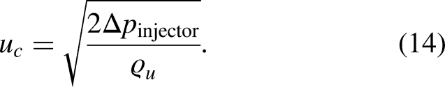
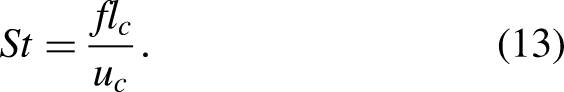
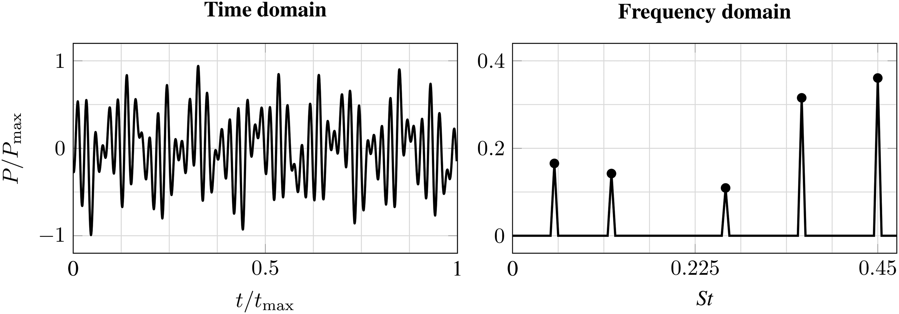
The acoustic excitation signal is included in Figure 7 in the time and frequency domains, in terms of the non-dimensional Strouhal number St. The Strouhal number is defined as the ratio of frequency $f$ and characteristic length $l_{c}$ to a characteristic velocity $u_{c}$

St = \frac{f l_{c}}{u_{c}}

(13)

The characteristic length is set to the diameter of the fuel injector,

l_{c} = D_{injector}

, and the characteristic velocity is defined using the pressure drop over the injector,

u_{c} = \sqrt{\frac{2 Δ p_{injector}}{ϱ_{u}}}

(14)

Figure 7.

Excitation signal for the numerical simulations in time and frequency domain. The signal comprises five tones that follow closely the experimental signals.

Discretization

One main advantage of the hybrid CFD-CAA approach is the possibility to tailor the numerical schemes to different physical domains. As such, it is important to introduce properly the spatial and temporal discretizations used in the context of this work. This section will introduce the different spatial domains used for SAS, LES, and CAA, as well as the applied temporal resolution.

Spatial discretization

In this work, two different numerical schemes are used with respect to turbulence resolution: an SAS computation with low-resolution spatial discretization, and a high-resolution LES computation. The SAS computations follow a tetrahedral, unstructured spatial discretization with $\sim$ 1.5 million control volumes. It is refined near the injector to allow for sufficient resolution of the combustion zone. A mesh of this size was used in previous work for non-reacting simulations, geometry investigation, and comparison to CAA,²³ and for a general but inexpensive validation of the hybrid SAS-CAA approach.²² More information on that mesh can be found in the respective publication by the authors.

For the compressible and low-Mach LES, a fully structured hexahedral mesh consisting of $\sim$ 11.5 million control volumes was used. A minimum edge length of $\sim$ 0.1 mm near the injector ensures a good resolution of the turbulent shear layers created in the wake of the injector. A section of the LES grid is presented in the top half of Figure 6. The injector itself is not presented due to confidentiality. To visualize the spatial discretization of the hybrid CAA, the mesh used in this study is displayed in the bottom half of Figure 6. For acoustic simulations of the thermoacoustic response behavior of an aero-engine combustor, the frequencies of interest are usually in a lower frequency range, for example, in this work, up to 1000 Hz. With lower frequencies corresponding to longer wavelengths, the maximum cell size of the CAA domain is limited by resolving the minimum wavelength of interest adequately. At the frequencies and temperatures of interest, this corresponds to $λ_{m i n} \approx$ 0.5 m in the duct upstream of the combustion chamber as the minimum wavelength that has to be resolved by the CAA mesh, thus allowing for a coarse spatial representation.

Temporal discretization

In addition to the strikingly different length scales, the hybrid CFD-CAA approach also uses a separation of time scales. This allows for the CFD timescale to be set to ensure a convective CFL number of less than unity for an accurate resolution of the convective dynamics. Meanwhile, the time step in the explicit CAA solver is chosen such that the acoustic CFL number is well below 0.5 in the entire domain. For the case under consideration, the frequencies of interest are comparatively low; hence, the acoustic CFL number is kept mostly below unity for the compressible LES at the same time step. In this work, the time scales for compressible and incompressible CFD simulations are kept identical, while the CAA time step is smaller by a factor of 100.

Results

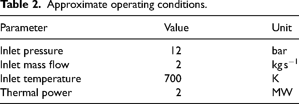
This work is a direct continuation of previous work that first implemented a hybrid, runtime-coupled CFD-CAA method for the computationally effective computation of thermoacoustic instabilities in aero-engine combustors. To this end, it will be validated against a high-fidelity compressible LES that has already shown excellent agreement with FTFs obtained via optical measurements.²⁵ The operating condition under investigation is therefore kept the same. Approximate values for pressure, mass flow, temperature, and thermal power for that configuration are listed in Table 2.

Table 2.

Approximate operating conditions.

Parameter	Value	Unit
Inlet pressure	12	bar
Inlet mass flow	2	kg s⁻¹
Inlet temperature	700	K
Thermal power	2	MW

First, the non-excited reacting simulations of compressible and low-Mach LES will be compared. Deviations already in the non-forced cases can be indicative of differences in the later post-processed acoustic quantities. Then, the acoustically forced simulations will be post-processed by means of the FTF, defined by the global heat release fluctuations and the acoustic velocity fluctuations. Finally, the necessary computational resources for the two approaches will be compared, making this the first quantitative assessment of possible savings in computing hours.

Non-excited LES

Using the same code basis PRECISE-UNS for compressible LES and hybrid LES-CAA facilitates directly comparing the results. To get a rough impression of the differences using the two formulations, non-forced reacting LES have been conducted and time-averaged over a long sampling duration, that is, at least 0.2 s physical time. Some mean flow field quantities (axial velocity ${\bar{u}}_{ax}$ , density $\bar{ϱ}$ , and temperature $\bar{T}$ ) are then plotted over the centerline of the SCARLET rig in Figure 8. Since the line plots are extracted from the centerline of SCARLET, the downstream duct quantities are largely influenced by an exhaust tube vortex towards the exit of the combustion chamber. The vortex is more pronounced in the compressible LES, and is maintained until the exit of the computational domain. Additionally, as evident from the plots, the upstream density values of both formulations do not agree. The mean upstream density is directly used to evaluate the FTF. Moreover, the temperature in the downstream duct of the compressible LES displays significantly higher values. This originates from higher combustion temperatures already in the combustor, and indicates differences in the combustion dynamics in both simulations.

Figure 8.

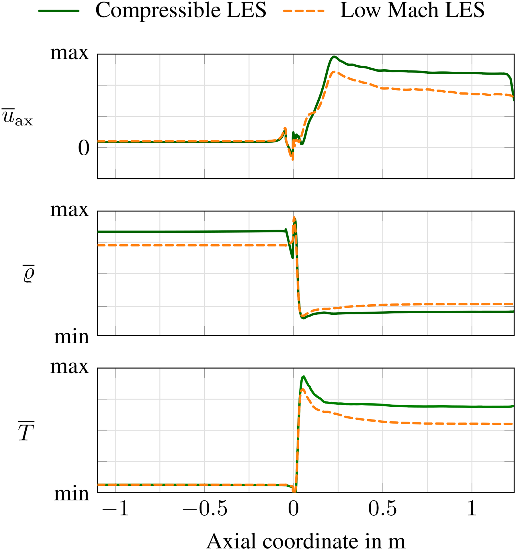
Time-averaged values for (top) axial velocity ${\bar{u}}_{ax}$ , (middle) density $\bar{ϱ}$ , and (bottom) temperature $\bar{T}$ , plotted over the centerline of the Scaled Acoustic Rig for Low Emission Technology (SCARLET).

General characteristics of the flow field

This section will describe the general flow features of the lean-burn SCARLET combustor at the investigated operating condition. It will use contour plots extracted from non-excited LES simulations of both the compressible and the low-Mach formulation of PRECISE-UNS at the same operating condition. As already discussed, the flow fields show some differences between the approaches, cf. Figure 8.

In Figure 9, the compressible and low-Mach time-averaged contours of the axial velocity component, temperature, local heat-release rate, and mixture fraction are provided in the top and the bottom halves of the pictures, respectively. In Figure 10, the instantaneous and time-averaged contours of the same quantities are provided, all extracted from the low-Mach LES.

Figure 9.

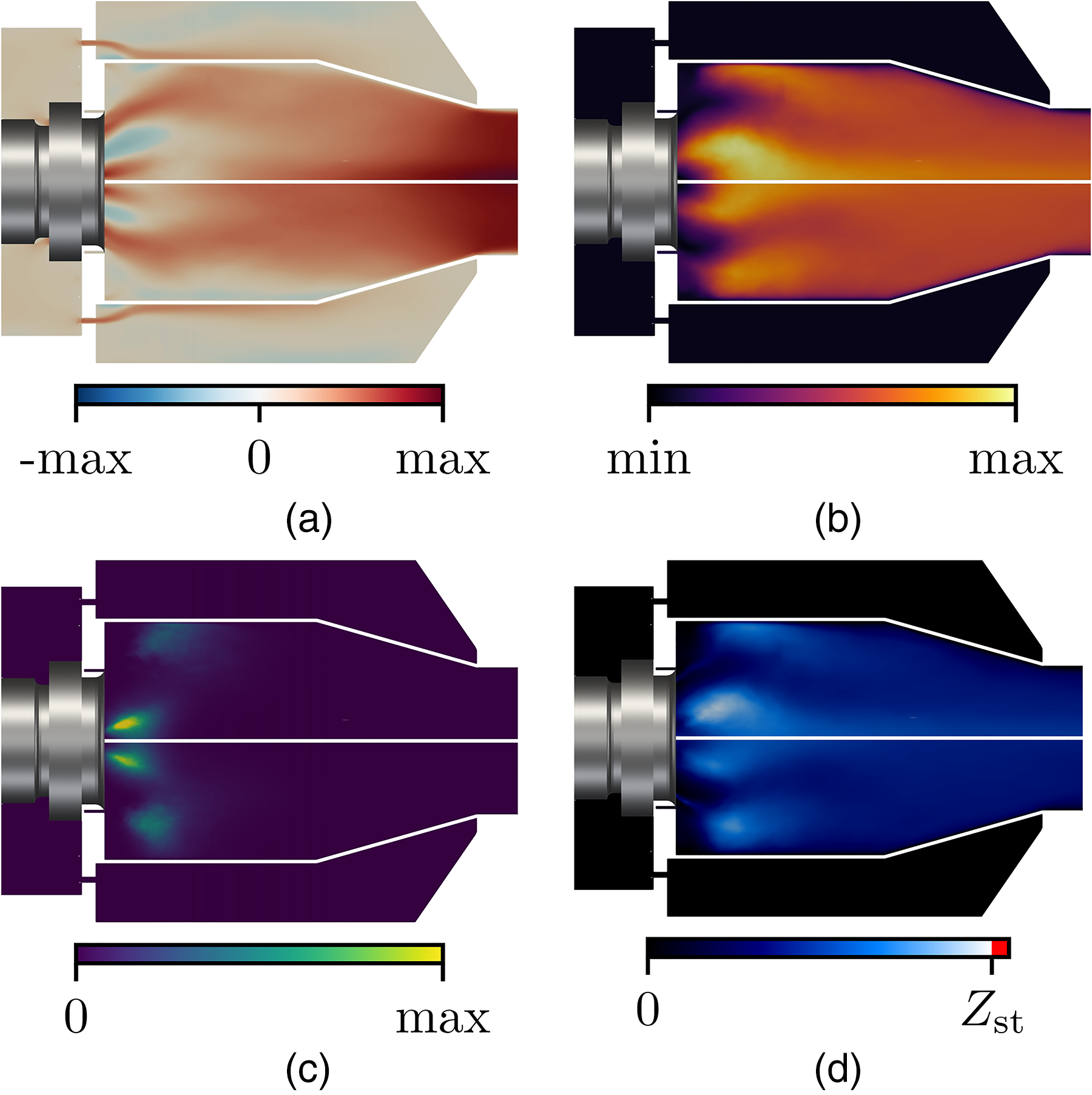
(Top) compressible and (bottom) low-Mach time-averaged flow quantities obtained from large eddy simulation (LES). Z_st denotes the stoichiometric mixture fraction. (a) Axial velocity; (b) temperature; (c) local heat-release rate; and (d) mixture fraction.

Figure 10.

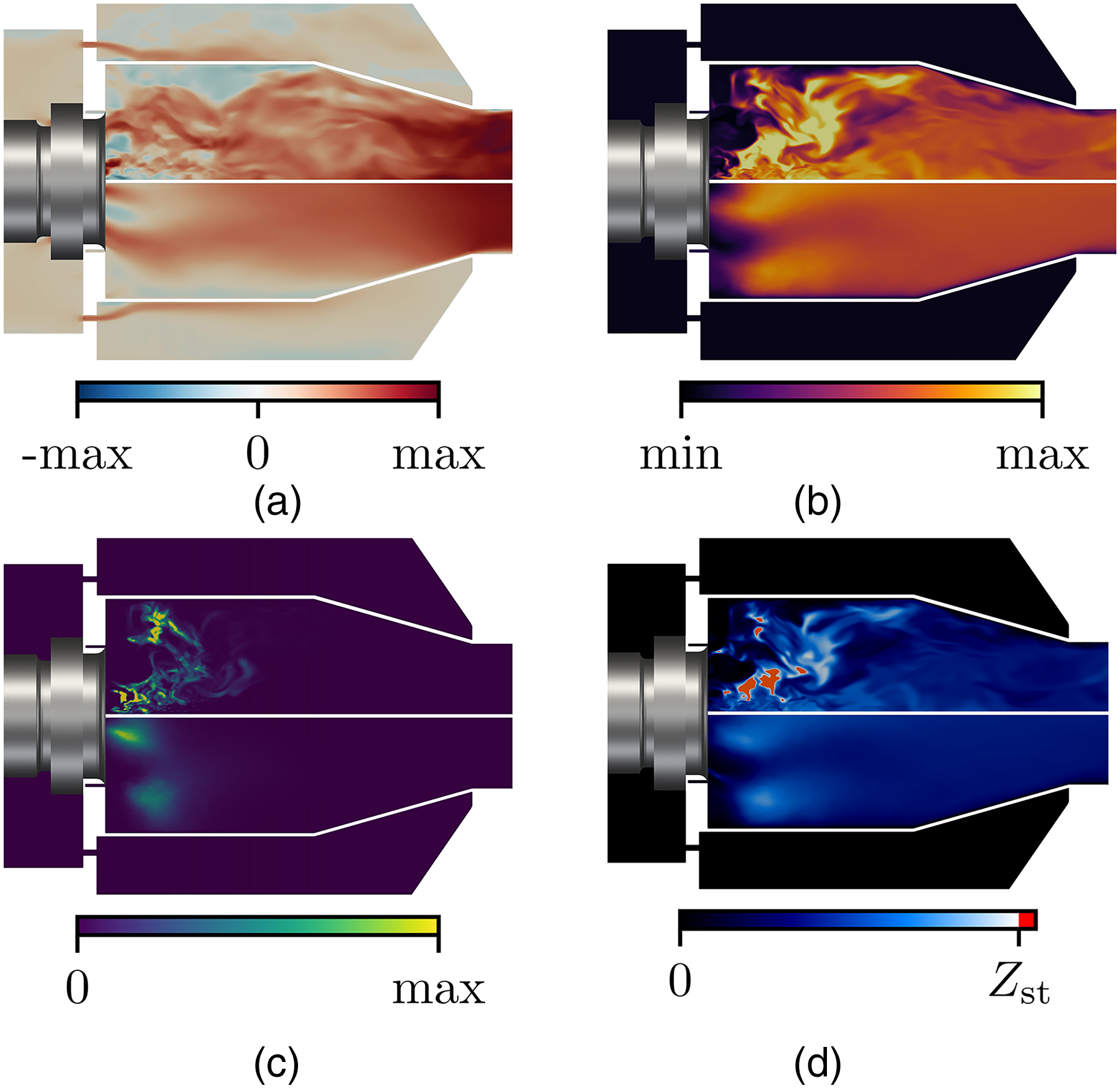
(Top) instantaneous and (bottom) time-averaged flow quantities obtained from incompressible LES. Z_st denotes the stoichiometric mixture fraction. (a) Axial velocity; (b) temperature; (c) local heat-release rate; and (d) mixture fraction.

Due to the geometry of the injector with three fluid flow passages and two circular injection zones, the flow in the combustion chamber splits into two areas: a pilot zone is characterized by high axial velocities towards the center of the combustion chamber, entrained by a recirculation zone, depicted with negative velocity values in Figures 9(a) and 10(a). The outer passages of the injector form a second zone of high axial velocity around the recirculation zone counter-rotating to the pilot jet, directed towards the effusion cooling liner. The flow is accelerated towards the exit of the combustion chamber due to thermal expansion. In the downstream duct, the velocity profile is rather homogeneous. The acceleration towards the combustor exit is even more pronounced in the compressible LES, and the exhaust vortex reaches deeper into the combustion chamber, and is maintained through the entire downstream duct, cf. Figure 10(a). In the compressible LES, the exit velocity of the injector is slightly higher than in the low-Mach simulation, which leads to higher velocities near the effusion liner and a noticeably bigger recirculation zone between the inner and outer passages. It should be noted that, even though the low-Mach approximation is valid due to the Mach numbers being well below 0.3 for most of the domain, the Mach number approaches this threshold in some cells in the jet emanating from the injector, possibly causing the marginal differences in the contour plots.

The mean temperature profiles displayed in Figure 10(b) provide a good idea of the flame structure within the combustion chamber, with the largest temperature gradient illustrating the flame location. The pilot flame is situated between the two jets exiting the injector, while the main flame is observed more towards the liner. The temperature field within this plane of the compressible LES is generally higher than that of the low-Mach LES, which was also observed in the previous section, cf. Figure 8. The flame position is unchanged between compressible and low-Mach CFD. Caused by the exhaust tube vortex, higher temperature fluid is transported into and through the downstream duct, leading to a higher speed of sound and influencing the acoustic propagation in the downstream measurement section. The flame structure is also evident from the local heat-release rate and mixture fraction contours in Figure 9(c) and (d). As observed in the mean field of mixture fraction, the global combustion characteristics show a lean mixture, with the compressible LES showing slightly higher mixture fractions closer to stoichiometry, and a higher maximum heat-release rate. The location of the highest local heat-release rate for compressible LES is very slightly shifted in the downstream direction. Following the more entrained flow field of the axial velocity, the main flame in the low-Mach LES is positioned closer behind the injector, and located further away from the effusion liner. Finally, the instantaneous field of the mixture fraction displays the mixing characteristics of the configuration, with fuel-rich pockets highlighted in red color (Figure 10(d)).

Acoustic characterization of the configuration

In the context of this work, the FTF is used as the main comparison between compressible and hybrid approaches. The evaluation of the FTF follows the definition already provided in equation (8). In the simulations, the acoustic excitation is introduced into the domain via the inlet boundary. To verify the influence of the acoustic excitation on the flow field of different approaches, the pressure spectra inside the upstream duct at the microphone positions are averaged and plotted in Figure 11. The black circles indicate the tones of the excitation signal as specified at the inlet for both approaches. The figure shows good agreement of the two spectra computed from the two approaches, and a close value to the excitation signal. 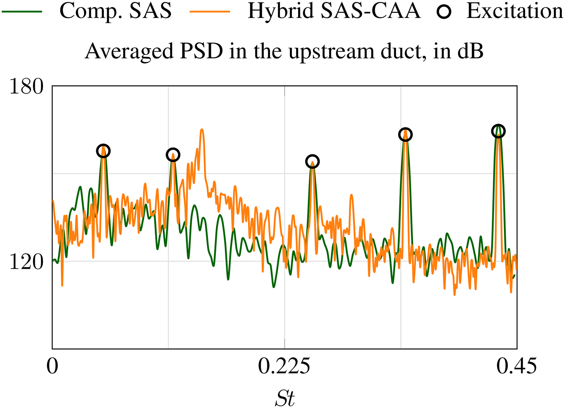Compared to the compressible SAS, the hybrid SAS-CAA plotted in Figure 11 shows a pressure mode at a Strouhal number of approximately $S t = 0.15$ . The observed resonance frequency at given speed of sound in the upstream duct corresponds to exactly one acoustic wave length that fits into the upstream duct. This indicates a higher reflectivity of the SAS-CAA at the combustion chamber inlet when compared with the compressible simulation, where this mode could not be observed. This mode is, however, close in frequency to a mode also observed in the experiment for this operating condition.

Figure 11.

Pressure spectrum from (orange) hybrid SAS-CAA and (green) compressible SAS. Circles indicate the excitation tones. SAS: scale-adaptive simulation; CAA: computational aeroacoustics.

Flame transfer function

After having noted that the general reaction of the two approaches to acoustic excitation is similar, this section will focus on directly comparing the FTFs. Compressible SAS and LES have shown mostly good agreement with the experiment, albeit not necessarily for the same frequencies (cf. Figure 5). The numerical framework for the simulation approaches differ in two main aspects: For the hybrid CFD-CAA simulations, a low-Mach CFD formulation is used, and the acoustics are attended to in a dedicated CAA solver. Since the acoustic simulation for the two considered hybrid CFD-CAA cases is kept the same, only the CFD parts differ. It is therefore intuitive that the hybrid SAS/LES-CAA simulations can at best be compared with the compressible counterparts, whereas the experiment can be used for comparison with and validation of the compressible simulation results.

In the following sections, the aforementioned SAS and LES will be analyzed and the FTFs of the different numerical approaches will be compared. The experimental FTF will always be provided in addition to the numerical FTF. It will, however, not be considered as comparison for—in particular—the hybrid simulation approach.

Scale-adaptive simulations

Figure 12 displays the FTFs for computationally less expensive SAS with both the compressible and the hybrid approach. For technically premixed flames with stiff fuel injection, the gain of the FTF should theoretically approach zero.⁴⁵ This is in stark contrast to the experimental value, and also to the numerical simulations using SAS modeling. The gain values of the compressible SAS and the hybrid SAS-CAA, however, show very good agreement over the entire frequency range, with only the second highest frequency showing less acoustic damping for the compressible SAS, manifested in a higher FTF gain.

Figure 12.

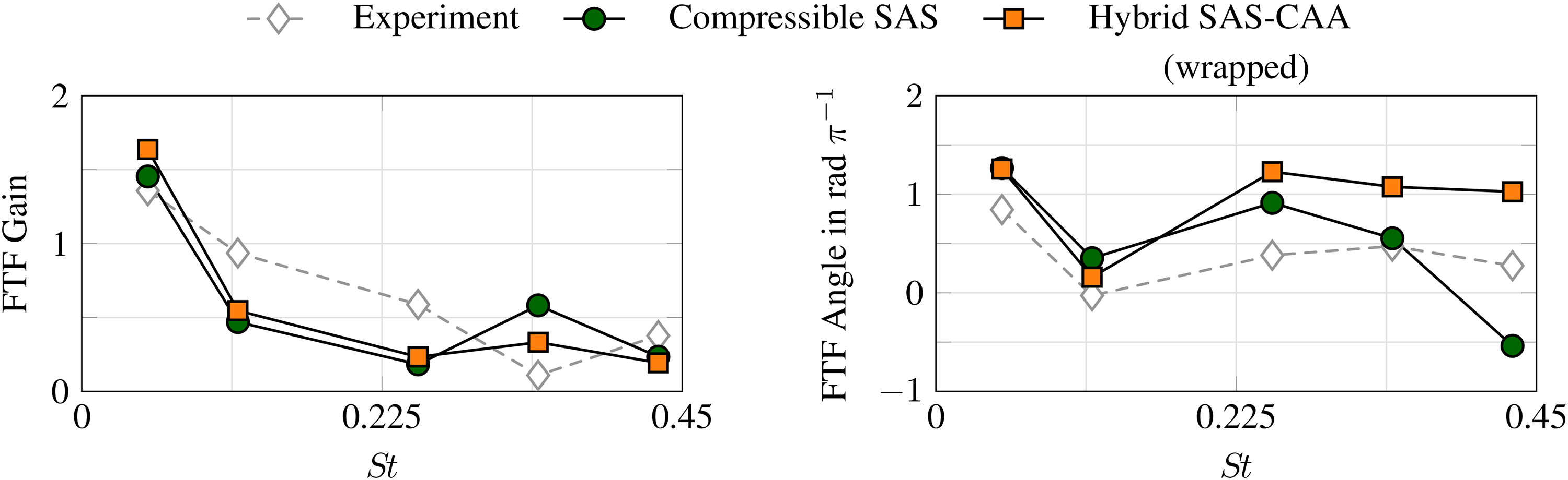
Flame transfer function from (circles) the compressible SAS and (squares) the hybrid SAS-CAA. SAS: scale-adaptive simulation; CAA: computational aeroacoustics.

The right side of Figure 12 displays the phase angles of the FTFs obtained from the SAS results. They are displayed, as they were in Figure 5, with values wrapped to $[- π, 2 π]$ . The phase angle of the FTF is considered a good measure of the convective dynamics of the acoustic system. For SAS, especially the lower frequency values show very similar behavior for compressible and hybrid simulation approaches, with the first frequency value $\sim$ $0.5 π$ higher than the experimental phase value. Theoretically, the zero-frequency limit $f \to 0$ of the FTF angle should be $\pm π$ ,⁴⁵ indicating that both numerical approaches overestimate the phase shift between input and output signals. For higher frequencies, the phase angle value for the compressible results is almost 1.5 $π$ shifted to the phase angle value of the hybrid SAS-CAA.

In addition to the gain values of the two FTFs generally showing a good agreement, the phase angle values of the compressible SAS and the hybrid SAS-CAA agree mostly well. Especially towards the lowest frequencies, the phase values are virtually identical. The slope between the frequency values, indicative of the time lags in the system, is particularly well recovered compared to the experimental values for the lower frequencies for the compressible SAS. Between the two highest frequency values in the experiment, the slope of the phase curve is very moderate compared to the lower frequencies. This change in slope is also obtained in the hybrid SAS-CAA, whereas the slope of the compressible SAS shows the most significant difference for the highest frequency.

Summarizing the results of the low-resolution CFD setups, the direct comparison between compressible SAS and hybrid SAS-CAA shows very good agreement, underlining that the general physics captured by the numerical approaches match well. While the agreement between the numerical approaches and the experiment in terms of the absolute values of the FTF gain is marginal for most frequencies, the numerical methods produce very similar results.

Overall, the results for the hybrid SAS-CAA are very encouraging and could indicate that the separation of fluid flow and acoustics can be a viable alternative to compressible SAS for capturing acoustics in such a low-resolution CFD setup. An assessment of the computational effort will be presented at the end of this work.

In the following section, this work will investigate the changes to the FTF if obtained using LES computations.

Large eddy simulations

In Figure 13, the compressible LES and the hybrid LES-CAA are compared, again in terms of the gain and the phase angle values of the FTF.

Figure 13.

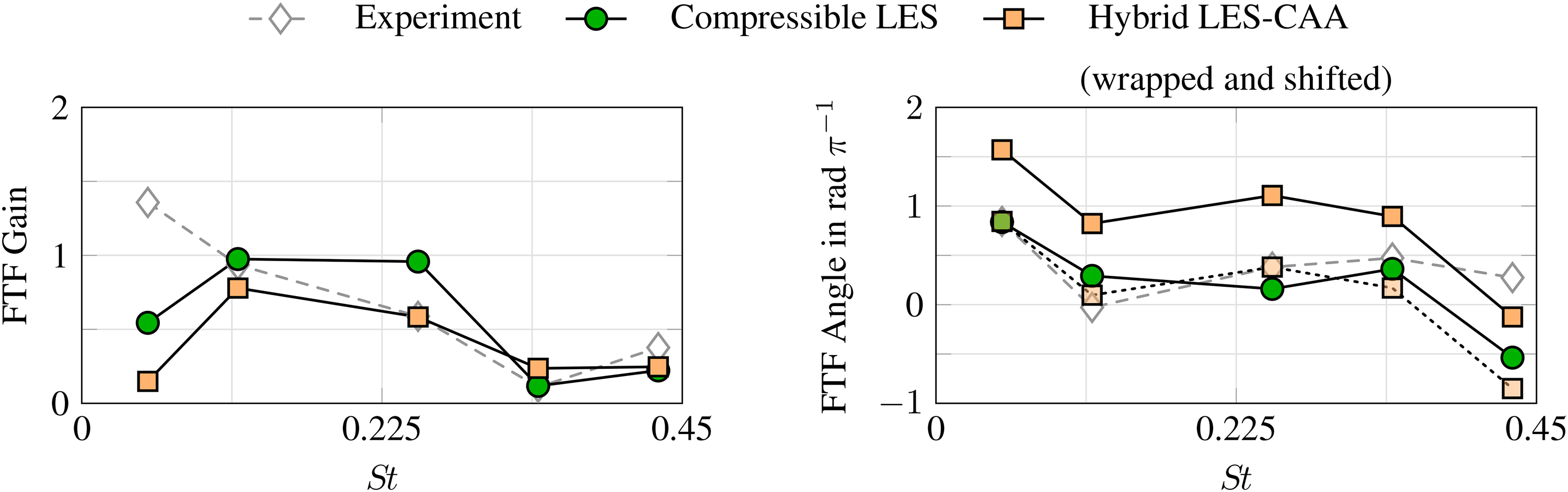
Flame transfer function from (circles) the compressible LES and (squares) the hybrid LES-CAA. The phase angle values from the hybrid LES-CAA (connected using dotted lines) are additionally shifted with respect to the original signal by $\sim$ $-$ 0.75 to coincide with the first phase angle value of the compressible LES. LES: large eddy simulation; CAA: computational aeroacoustics.

Considering the gain of the FTF displayed on the left side, both compressible LES and hybrid LES-CAA show significant changes when compared to the respective SAS. The general shape of the FTF gain agrees well between compressible LES and hybrid LES-CAA. However, they overall deviate more from each other for most frequencies. Compared to the SAS results, the lowest frequencies differ most significantly, with the first frequency value approaching zero in the LES, while the gain values for SAS were greater than 1. The higher frequency values are not only very close to the experimental reference, but also mirror the general trend of the gain. Since low frequencies usually are most sensitive to sampling errors, it is a common observation to have most significant deviations in lower frequencies.

The phase angle values are displayed on the right-hand side of Figure 13. At the lowest frequency, compressible LES and experiment match perfectly, while the hybrid LES-CAA displays a significant phase shift of $\sim$ 0.75. Besides the vertical offset of the phase angle values, compressible LES and hybrid LES-CAA display a similar convective behavior in that the phase angle sloped between neighboring frequency values mostly agree well. They retain a similar value for the mid-frequency range, and display a steep decline for the two highest frequencies. Considering the general good agreement in phase angle slope between compressible and hybrid approaches, it is conceivable that the vertical offset results from a different temporal reference when sampling the signals, but the general physics that are described are the same.

In summary, every comparison between compressible CFD and hybrid CFD-CAA has mostly shown good agreement for a significant number of tones, at least displaying similar trends in gain and phase of the FTF. Due to the high complexity and large number of unknowns in the considered configuration, deviations persist. Especially with respect to the low-frequency limit of the FTF, additional investigation would be necessary to conclude the root cause of the differences.

Evaluating the computational efficiency

After demonstrating that both compressible and hybrid simulations can capture the FTF of the considered configuration, this section will finally compare the computational costs for all cases presented here. All computations were performed on the Lichtenberg High-Performance Computer at Technical University of Darmstadt. For the comparison of computational cost, the presented simulations were conducted using $\sim$ 200 cores for the respective CFD simulation. The computational effort is then compared in terms of relative CPU hours (CPUh), which is graphically displayed in Figure 14.

Figure 14.

Comparison of relative CPU hours (CPUh) for low-Mach CFD, hybrid CFD-CAA and compressible CFD for both SAS and LES. The values given are relative to the respective low-Mach simulation. (a) SAS: scale-adaptive simulation; (b) LES: large-eddy simulation.

The relative CPUh are defined with the necessary resources for the respective reacting, non-excited low-Mach CFD simulation. Compared to the low-Mach CFD simulation, the hybrid computation includes the receiving and sending of acoustic and flow quantities, respectively, and additional steps to reflect the acoustic fluctuations in the density, pressure, and velocity calculation. For the SASs (Figure 14(a)) and the LESs (Figure 14(b)), the general trend of the necessary computing resources remains similar. Because of the additional physics involved, both hybrid and compressible approaches are naturally more computationally expensive than the respective low-Mach counterparts. Since the CFD simulations mostly use the same simulation framework bar the compressible extensions, this comparison marks the closest juxtaposition to evaluate the computational efficiency.

As shown in Figure 14, especially for the SAS computations, the hybrid CFD-CAA method exhibits lower cost in terms of the necessary computing resources. While the compressible simulation almost doubles the resources necessary for the low-Mach CFD, the hybrid CFD-CAA only marks an increase of 28%. For the LES, the computational effort for the two acoustic simulations is closer in terms of relative CPUh. Future applications of the bidirectional coupling of CFD and CAA could explore ways to further decrease the computational overhead of the coupling mechanism, as well as examine the improvement of the compressible LES and its implications.

Conclusion

In this work, a hybrid LES-CAA method was applied to a realistic single-sector aero-engine combustor configuration, and the results were discussed in comparison to both compressible LES and experimental data. Insight into the thermoacoustic behavior of the system was gained by capturing acoustic and heat-release rate fluctuations, and relating them to obtain the FTF for a given liquid fuel injector. The main objective was directly comparing the hybrid, runtime-coupled CFD-CAA method to conventional compressible CFD simulations, and assessing the computational costs.

The thermoacoustic response of all simulations in terms of the FTF was assessed, concluding that the FTF evaluated from the hybrid CFD-CAA simulations showed very close agreement with the direct compressible reference. The consensus between the two numerical approaches allows the conclusion that the hybrid CFD-CAA approach can be a promising alternative to the conventional compressible CFD simulations, describing a similar flame response.

This conclusion can be strengthened by the comparison of the respective computational effort for compressible CFD and hybrid CFD-CAA simulations. For the configurations described in this work, the relative computational time needed for the hybrid approach was lower than for the compressible simulations, especially for SAS turbulence modeling in the CFD solver.

In summary, this work has demonstrated that the implemented bidirectional and runtime coupling of low-Mach CFD and CAA can capture the acoustic behavior of a complex combustion system similarly to compressible CFD. In addition to resulting in very similar FTFs, the computational effort necessary for the hybrid CFD-CAA method is lower than that of compressible simulations.

Footnotes

Acknowledgements

The investigations in this work were conducted as part of the joint research program Kosten- und leistungsoptimierte Brennkammer-Turbinentechnologien für moderne Turbo-Generatoren (OptTuGen) under the scheme “Luftfahrtforschungsprogramm LuFo VI-3” on the basis of a resolution of the German Bundestag. It is financially supported by the Federal Ministry for Economic Affairs and Climate Action (BMWK) under grant number 20M2264B.

The authors gratefully acknowledge the computing time provided to them on the high-performance computer Lichtenberg at the NHR Centers NHR4CES at TU Darmstadt. This is funded by the Federal Ministry of Education and Research, and the state governments participating on the basis of the resolutions of the GWK for national high performance computing at universities ().

Finally, the authors want to express their gratitude to Ruud Eggels and Max Staufer from Rolls-Royce Deutschland for their ongoing support.

Declaration of conflicting interests

The author(s) declare no potential conflicts of interest with respect to the research, authorship, and/or publication of this article.

Funding

The author(s) received no financial support for this article’s research, authorship, and/or publication.

ORCID iDs

Hanna Reinhardt

Çetin Ozan Alanyalıoğlu

References

European Commission and Directorate-General for Mobility and Transport and Directorate-General for Research and Innovation. Flightpath 2050: Europe’s Vision for Aviation: Maintaining Global Leadership and Serving Society’s Needs. Publications Office, 2012. DOI: 10.2777/15458.

Lefebvre

Ballal

. Gas Turbine Combustion. Boca Raton, FL: CRC Press, 2010. DOI: https://doi.org/10.1201/9781420086058.

Lieuwen

Yang

. Combustion Instabilities in Gas Turbine Engines. Reston, VA: American Institute of Aeronautics and Astronautics, 2006. DOI: https://doi.org/10.2514/4.866807.

Dowling

Mahmoudi

. Combustion noise. Proc Combust Inst 2015; 35: 65–100. DOI: https://doi.org/10.1016/j.proci.2014.08.016 .

Tay-Wo-Chong

Bomberg

Ulhaq

et al. Comparative validation study on identification of premixed flame transfer function. J Eng Gas Turbine Power 2012; 134: 021502. DOI: https://doi.org/10.1115/1.4004183 .

Krediet

Beck

Krebs

et al. Saturation mechanism of the heat release response of a premixed swirl flame using LES. Proc Combust Inst 2013; 34: 1223–1230. DOI: https://doi.org/10.1016/j.proci.2012.06.140 .

Meindl

Merk

Fritz

et al. Determination of acoustic scattering matrices from linearized compressible flow equations with application to thermoacoustic stability analysis. J Theor Comput Acoust 2019; 27: 1850027. DOI: https://doi.org/10.1142/S2591728518500275 .

Merk

Silva

Polifke

et al. Direct assessment of the acoustic scattering matrix of a turbulent swirl combustor by combining system identification, large eddy simulation and analytical approaches. J Eng Gas Turbine Power 2019; 141: 021035. DOI: https://doi.org/10.1115/1.4040731 .

Bui

Schröder

Meinke

. Acoustic perturbation equations for reacting flows to compute combustion noise. Int J Aeroacoustics 2007; 6: 335–355. DOI: https://doi.org/10.1260/147547207783359468 .

10.

Gikadi

Ullrich

Sattelmayer

et al. Prediction of the acoustic losses of a swirl atomizer nozzle under non-reactive conditions. In: ASME Turbo Expo 2013: Turbine Technical Conference and Exposition. American Society of Mechanical Engineers. DOI: 10.1115/GT2013-95449.

11.

Klewer

Ketelheun

Janicka

. Numerical analysis of thermoacoustic instabilities using LES and computational aeroacoustics. Zeitschrift für Physikalische Chemie 2011; 225: 1393–1403. DOI: https://doi.org/10.1524/zpch.2011.0186 .

12.

Andreini

Facchini

Giusti

et al. Assessment of flame transfer function formulations for the thermoacoustic analysis of lean burn aero-engine combustors. Energy Procedia 2014; 45: 1422–1431. DOI: https://doi.org/10.1016/j.egypro.2014.01.149 .

13.

Ullrich

Hirsch

Sattelmayer

et al. Combustion noise prediction using linearized Navier-Stokes equations and large-eddy simulation sources. J Propuls Power 2017; 34. DOI: https://doi.org/10.2514/1.B36428 .

14.

Polifke

Poncet

Paschereit

et al. Reconstruction of acoustic transfer matrices by instationary computational fluid dynamics. J Sound Vib 2001; 245: 483–510. DOI: https://doi.org/10.1016/jsvi.2001.3594 .

15.

Föller

Polifke

. Identification of aero-acoustic scattering matrices from large eddy simulation. Application to a sudden area expansion of a duct. J Sound Vib 2012; 331: 3096–3113. DOI: https://doi.org/10.1016/j.jsv.2012.01.004 .

16.

Gentemann

AMG

. Identifikation von akustischen Transfermatrizen und Flammenfrequenzgängen mittels Strömungssimulation. Doctoral thesis, Technische Universität München, München, 2006.

17.

Lackhove

Sadiki

Janicka

. Efficient three dimensional time-domain combustion noise simulation of a premixed flame using acoustic perturbation equations and incompressible LES. In: ASME Turbo Expo 2017: Turbomachinery Technical Conference and Exposition. American Society of Mechanical Engineers. DOI: 10.1115/GT2017-63050.

18.

Ewert

Schröder

. Acoustic perturbation equations based on flow decomposition via source filtering. J Comput Phys 2003; 188: 365–398. DOI: https://doi.org/10.1016/S0021-9991(03)00168-2 .

19.

Bui

Schröder

Meinke

et al. Source term evaluation of the APE-RF system using DNS data. In: Proceedings of the European Conference on Computational Fluid Dynamics. Delft University of Technology. DOI: 10.2514/6.2006-2678.

20.

Geiser

Nawroth

Hosseinzadeh

et al. Thermoacoustics of a turbulent premixed flame. In: 20th AIAA/CEAS Aeroacoustics Conference. American Institute of Aeronautics and Astronautics. ISBN 978-1-62410-285-1. DOI: 10.2514/6.2014-2476.

21.

Reinhardt

Alanyalıoğlu

ÇO

Fischer

et al. A hybrid, runtime coupled incompressible CFD-CAA method for analysis of thermoacoustic instabilities. J Eng Gas Turbine Power 2023; 145: 031003. DOI: https://doi.org/10.1115/1.4055666 .

22.

Reinhardt

Alanyalıoğlu

ÇO

Fischer

et al. Simulation of the thermoacoustic response of an aero-engine gas turbine fuel injector using a hybrid CFD-CAA method. J Eng Gas Turbine Power 2023; 145: 111016. DOI: https://doi.org/10.1115/1.4063335 .

23.

Alanyalıoğlu

ÇO

Reinhardt

Fischer

et al. Acoustic scattering behaviour of an aero engine injector: Numerical investigation using compressible CFD and CAA. In: Proceedings of the ASME Turbo Expo 2022: Turbomachinery Technical Conference and Exposition. Turbo Expo: Power for Land, Sea, and Air, American Society of Mechanical Engineers. DOI: 10.1115/GT2022-82901.

24.

Treleaven

NCW

Fischer

Lahiri

et al. The effects of forcing direction on the flame transfer function of a lean-burn spray flame. In: ASME Turbo Expo 2021: Turbomachinery Technical Conference and Exposition. American Society of Mechanical Engineers. DOI: 10.1115/GT2021-59553.

25.

Alanyalıoğlu

ÇO

Reinhardt

Fischer

et al. Analysis of the thermo-acoustic response of an aero-engine injector using compressible LES. In: Proceedings of the 15th European Conference on Turbomachinery Fluid Dynamics and Thermodynamics. DOI: 10.29008/ETC2023-376.

26.

Anand

Eggels

RLGM

Staufer

et al. An advanced unstructured-grid finite-volume design system for gas turbine combustion analysis. In: ASME 2013 Gas Turbine India Conference. American Society of Mechanical Engineers. DOI: 10.1115/gtindia2013-3537.

27.

Klapdor

di Mare

Kollmann

et al. A compressible pressure-based solution algorithm for gas turbine combustion chambers using the PDF/FGM model. Flow Turbul Combust 2013; 91: 209–247. DOI: https://doi.org/10.1007/s10494-013-9451-2 .

28.

Nicoud

Toda

Cabrit

et al. Using singular values to build a subgrid-scale model for large eddy simulations. Phys Fluid 2011; 23: 085106. DOI: https://doi.org/10.1063/1.3623274 .

29.

Menter

Egorov

. The scale-adaptive simulation method for unsteady turbulent flow predictions. Part 1: Theory and model description. Flow, Turbulence Combust 2010; 85: 113–138. DOI: https://doi.org/10.1007/s10494-010-9264-5 .

30.

Jasak

Weller

Gosman

. High resolution NVD differencing scheme for arbitrarily unstructured meshes. Int J Numer Methods Fluids 1999; 31: 431–449. DOI: https://doi.org/10.1002/(SICI)1097-0363(19990930)31:2¡431::AID-FLD884¿3.0.CO;2-T

31.

Cantwell

Moxey

Comerford

et al. Nektar++: an open-source spectral/hp element framework. Comput Phys Commun 2015; 192: 205–219. DOI: https://doi.org/10.1016/j.cpc.2015.02.008 .

32.

Lackhove

. Hybrid Noise Simulation for Enclosed Configurations. Doctoral thesis, Technische Universität Darmstadt, Darmstadt, 2018.

33.

Quémerais

. La Bibliothèque de Couplage CWIPI — Coupling With Interpolation Parallel Interface, 2018. https://w3.onera.fr/cwipi/bibliotheque-couplage-cwipi.

34.

Fischer

Lahiri

Dörr

. Thermoakustik mager betriebener Brennkammern - Untersuchungen am SCARLET Prüfstand. In: 16. Statusseminar der AG Turbo - Tagungsband. Wissenschaftliche Koordinierungsstelle AG Turbo.

35.

Fischer

Lahiri

. Ranking of aircraft fuel-injectors regarding low frequency thermoacoustics based on an energy balance method. In: ASME Turbo Expo 2021: Turbomachinery Technical Conference and Exposition. American Society of Mechanical Engineers. DOI: 10.1115/GT2021-59561.

36.

Paschereit

Schuermans

Polifke

et al. Measurement of transfer matrices and source terms of premixed flames. In: ASME 1999: International Gas Turbine and Aeroengine Congress and Exhibition. American Society of Mechanical Engineers. DOI: 10.1115/99-GT-133.

37.

Lahiri

. Acoustic Performance of Bias Flow Liners in Gas Turbine Combustors. Doctoral thesis, Technische Universität Berlin, Fakultät V - Verkehrs- und Maschinensysteme, Berlin, 2014. DOI: 10.14279/depositonce-4270.

38.

Gebel

Fischer

. Schlussbericht Teil I und II zu: Fortgeschrittene Messmethoden der Verbrennungstechnik (AG Turbo 2020 - 2.3.4d). Project report, Rolls-Royce Deutschland, 2018.

39.

Poinsot

Lele

. Boundary conditions for direct simulations of compressible viscous flows. J Comput Phys 1992; 101: 104–129.

40.

van Oijen

de Goey

. Modelling of premixed laminar flames using flamelet-generated manifolds. Combust Sci Technol 2000; 161: 113–137. DOI: https://doi.org/10.1080/00102200008935814 .

41.

Hermanns

RTE

. CHEM1D, a one-dimensional laminar flame code. Report, Eindhoven University of Technology. 2001

42.

Karbach

Muharam

Riedel

et al. Reaktionsmechanismen flüssiger Kohlenwasserstoffe. In: Colloquium of COSI - Combustion Control and Simulation.

43.

Chin

Lefebvre

. Steady-state evaporation characteristics of hydrocarbon fuel drops. AIAA J 1983; 21: 1437–1443. DOI: https://doi.org/10.2514/3.8264 .

44.

Newman

. An L1 extremal problem for polynomials. Proc Am Math Soc 1965; 16: 1287. DOI: https://doi.org/10.2307/2035916 .

45.

Polifke

Lawn

. On the low-frequency limit of flame transfer functions. Combust Flame 2007; 151: 437–451. DOI: https://doi.org/10.1016/j.combustflame.2007.07.005 .