
Abstract
The computation of flame transfer functions (FTFs), which characterize the flame response to acoustic fluctuations, is of central importance to the assessment of thermoacoustic stability. Hydrogen is an important carbon-free fuel to ensure sustainable power production in gas turbines. Since hydrogen possesses different reactivity and thermo-diffusive characteristics in comparison to natural gas, the nominal flame structure is different from natural gas, and therefore it also exhibits different dynamics. In the context of computing hydrogen flames, the non-unity Lewis numbers call for transport models that consider the enhanced molecular diffusion of hydrogen. This article answers an open question of how present-day computational fluid dynamics (CFD) solvers and transport models perform in the calculation of flame dynamics. Computations of FTFs of laminar premixed hydrogen flames are performed using OpenFOAM, ANSYS Fluent, S3D DNS code, and the AVBP solver. These solvers encompass the spectrum of numerical schemes and transport models used in computational combustion. Transport models taking into account the enhanced molecular diffusion of hydrogen are used in each solver. The results show that despite using similar transport models and identical chemical mechanisms, quantitative differences in the laminar flame speed, mean flame shapes, and the FTFs are seen between the solvers. However, the qualitative features of the FTF remain the same and the quantitative differences in terms of the root-mean-square error metric are within
Keywords
Introduction
Combustion instability, an important practical problem in gas turbine and rocket engines, is caused due to the coupled interaction between the flame, flow, and the resonant acoustic modes of a combustion chamber.
1
Flames respond to acoustic waves by modulating their heat release rate, position, and shape
2
in time. Unsteady flames, in turn, act as a source of sound creating acoustic waves.
3
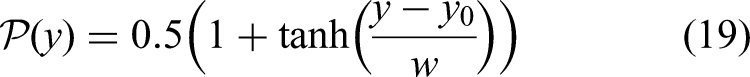
This coupled feedback loop involves an interplay between the intricate combustion, hydrodynamic, and acoustic phenomena and is generally non-trivial to predict. Insight into the thermoacoustic behavior of a given flame–combustion chamber system can be obtained by computing the open-loop response of the flame to acoustic perturbations. For this purpose, the flame is subjected to acoustic waves either experimentally using a loudspeaker/siren4,5 or numerically by imposing acoustic waves at the inlet/exit of the computational domain.6,7 The resulting global heat release response of the flame is measured/calculated to derive a flame transfer function (FTF) which can be mathematically written as
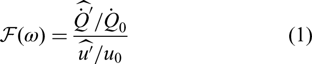
A FTF has a characteristic frequency
Hydrogen is regarded as a crucial carbon-free fuel that will play a key role in enabling power generation in gas turbine engines with low greenhouse gas emissions. However, it possesses different physical and chemical properties to that of natural gas, and therefore, must be re-assessed from the standpoint of combustion instability. In other words, the combustion (in)stability characteristics of existing burners must be re-evaluated when using hydrogen since it results in flames with nominally different shapes and heat release distributions. Two unique properties of hydrogen are particularly important in this regard. First, hydrogen exhibits an increased reactivity (increased laminar flame speed) in comparison to natural gas. For a fixed flow velocity and flame temperature, hydrogen flames are much shorter than natural gas flames, and this reflects in FTFs as a reduced phase slope and increased cutoff frequency.13–15 Additionally, hydrogen also exhibits enhanced diffusivities of mass in relation to heat, and therefore has a strong stretch/curvature sensitivity of the local consumption speed.16,17 For a fixed unstretched laminar flame speed and flow velocity, hydrogen flames can exhibit shorter or longer flame lengths in comparison to natural gas depending on the flame front curvature and the Markstein length. 18 Therefore, it is natural to expect, even under conditions where the flow velocity and the unstretched laminar flame speed are maintained constant, differences in the FTF of hydrogen and natural gas flames. This warrants the need for tools to computationally determine the FTFs of hydrogen flames to get insight into the combustion instability characteristics of these carbon-free fuels.
Since the enhanced mass diffusivity of hydrogen is a key characteristic of the fuel, computational approaches to extract the FTF of hydrogen flames must capture the non-unity Lewis numbers of hydrogen. More specifically, transport models that set all species Lewis numbers to unity, while working well for natural gas flames, are not expected to capture the physics of hydrogen flames. To consistently capture the enhanced mass diffusivity of hydrogen in a flame computation, three approaches are possible. First, a “multi-component” transport model where the species diffusional velocities are computed by solving a system of linear equations involving the binary diffusion coefficients
The importance of correctly capturing the enhanced mass diffusivity of hydrogen in computations of the static and dynamic flame characteristics prompts us to the following key question. How do different flow solvers and transport models compare in computing key combustion characteristics (static and dynamic) of hydrogen flames? Furthermore, we also intend to get quantitative insight into the relative differences in FTFs obtained when using different solvers and transport models. Answering the preceding research questions will be the main aim of this paper. To accomplish this, we perform computations of one-dimensional (1D) laminar premixed flames and two-dimensional (2D) slit-stabilized laminar premixed flame dynamics of hydrogen flames using different computational fluid dynamics (CFD) solvers and different transport models. While we acknowledge that the present study only focuses on laminar premixed flames, whereas real-world gas turbine combustors mostly feature turbulent flames, we emphasize that the current work represents a first step to understand how different flow solvers and transport models behave in computing hydrogen flames, and can be easily extended to turbulent premixed flames in the future. The computations in this work are performed using the open-source flow solvers OpenFOAM, 21 ANSYS Fluent v2024 R1, S3D DNS code of Sandia National Laboratories, 22 and the AVBP solver from CERFACS. 23 The next section gives details of the geometrical configuration and the computational methods employed.
Geometrical configuration and computational methodology
Both 2D and 1D computations of laminar premixed flames are performed in this work. While the 2D computations are used to characterize the flame shapes, global consumption speeds, and the flame dynamics, the 1D computations (see Figure 1) are intended to compute the unstretched laminar flame speeds. The 1D computations feature a premixed propagating flame and are simulated computationally using a three-dimensional domain with an axial extent of


One-dimensional geometrical configuration used for the unstretched laminar flame speed computations.
For the 2D computations, a slit-flame combustor (see Figure 2), originally introduced by Meindl et al.,
25
is employed. This configuration consists of a straight channel with a length of

Slit-flame configuration featuring a premixed propagation-stabilized flame. This configuration is used for characterizing the stretch-affected laminar flame speed and the flame dynamics.
OpenFOAM computational methodology
The reactingFOAM compressible solver from the OpenFOAM v1021,26 toolbox is used for computing the laminar premixed flame and its dynamics. Viscosity and thermal conductivity of each species are specified as polynomial functions of temperature. From these individual species viscosities, thermal conductivities, and the species mass fractions, the mixture-averaged viscosity and thermal conductivity are then calculated using standard mixture-averaging rules. 20 The mixture-specific heats and enthalpies are also computed from the corresponding species values, which are given in the form of NASA polynomials 27 as a function of temperature. The reacting mixture in OpenFOAM is specified as a “coefficientWilkeMultiComponentMixture” which implicitly implements the mixture-averaging rules.
A vital aspect in the computation of hydrogen flames is the representation of the enhanced mass diffusivities of hydrogen. This is done using a mixture-averaged (MA) transport model approach, which is incorporated using the “FickianFourier” utility in OpenFOAM. In this framework, the species diffusional velocities are calculated using the Fickian law,
28
which involves the spatial gradients of species mass (or mole) fractions and the mixture-averaged diffusion coefficients
Method used for computation of transport properties for the MA transport model in the various solvers.

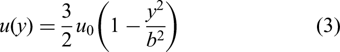
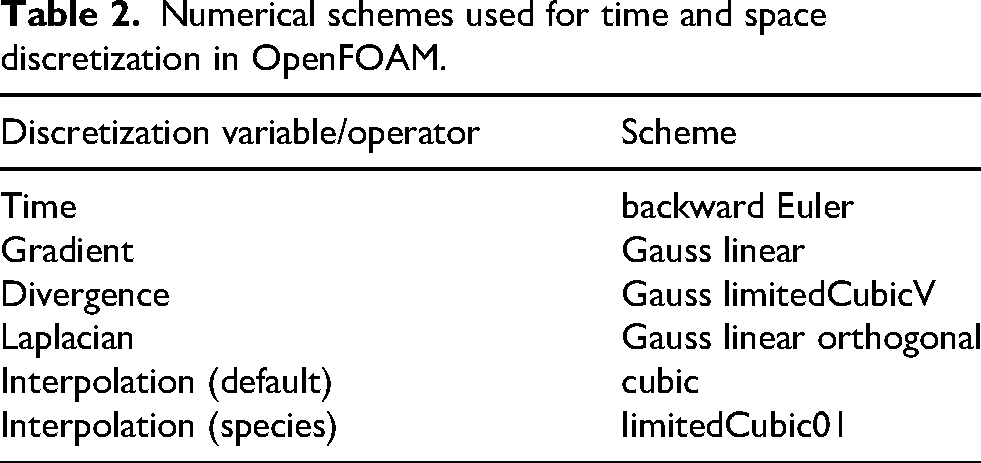
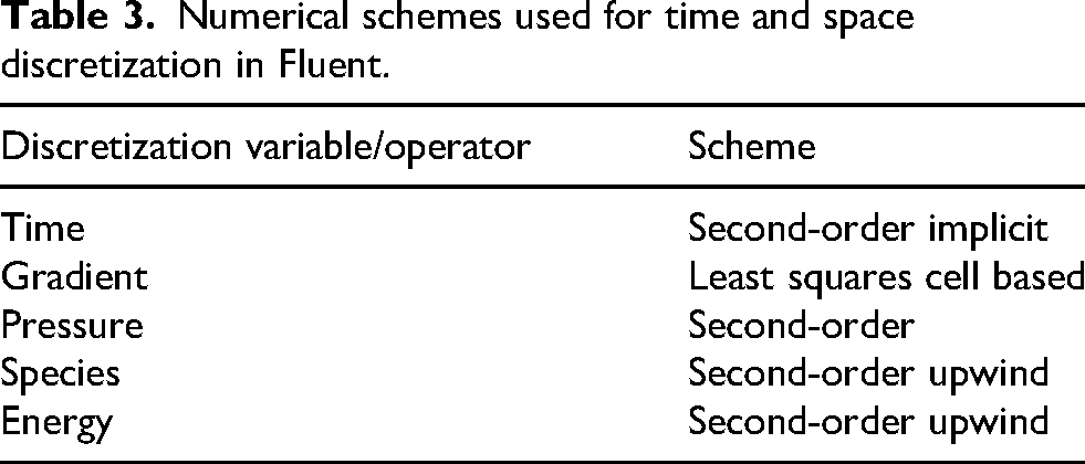
With regard to the boundary conditions imposed for the computations, at the inlet, the temperature and species mass fractions are specified as fixed values using the “fixedValue” type condition, and a “zeroGradient” condition is imposed for pressure. The parabolic velocity profile at the inlet is specified using the “codedFixedValue” condition. A “waveTransmissive” boundary condition is employed for the pressure at the outlet boundary, which imposes a partially non-reflective outflow in accordance with the Navier–Stokes characteristic boundary condition (NSCBC) methodology with a specified relaxation coefficient.29,30 This relaxation coefficient is specified as a length parameter (lInf) which is kept constant at 1 m for all computations reported in this paper. A “pressureInletOutletVelocity” condition is imposed for velocity at the outlet. No-slip isothermal/adiabatic condition is imposed at the walls, while the “symmetry” condition is employed for the bottom boundary. Except for the inlet, all the other boundaries employ a “zeroGradient” condition for species mass fractions. A PIMPLE algorithm with 15 outer iterations and 4 inner iterations is used for the computations. The numerical schemes employed for the temporal and spatial discretization are listed in Table 2. The maximum convective Courant–Friedrichs–Lewy (CFL) number is maintained as 0.4 for all the computations.
Numerical schemes used for time and space discretization in OpenFOAM.
AVBP computational methodology
AVBP is a massively parallel, fully compressible, reactive turbulent flow solver designed for both Large eddy simulations (LES) and direct numerical simulation (DNS) on GPU and CPU architectures. It solves the multi-species reactive Navier–Stokes equations in conservative form on both structured and unstructured grids, using a cell-vertex finite-volume method. 23 The viscous–convective part of the flux tensor is discretized with a revisited version of the multi-parameter family of a two-step Taylor–Galerkin (TTG) scheme, 31 denoted TTGC, 32 which is the third-order accurate both in space and time. Since AVBP is extensively employed for LES of industrial configurations, the scheme is designed to handle hybrid and irregular meshes without exhibiting over-dissipative behavior at high frequencies, which would otherwise damp important turbulent structures at practical mesh resolutions. At the same time, it achieves a near fourth-order accuracy in some norms for relatively regular meshes, 33 as is the case in the present work. On the other hand, the inviscid-diffusive part of the flux tensor is discretized with a centered second-order scheme. The acoustic CFL number, set to 0.7 in this work, is chosen by the user and kept below the critical CFL threshold of the convection scheme. This corresponds to a time-dependent time step of approximately 10 ns across all simulated cases.
The thermodynamic properties of the mixture are derived from the NIST–JANAF tables 27 or from the CHEMKIN database. 34 As far as the transport model is concerned, to adequately capture the enhanced mass diffusivity of hydrogen, a mixture-averaged approach is employed. This method provides a more accurate determination of transport coefficients by accounting for the composition-dependent contributions of each species in the mixture. The resulting transport properties correspond to those of a hypothetical mixture with averaged characteristics. According to the Chapman–Enskog theory,35,36 the evaluation of the mixture viscosity, thermal conductivity, and diffusivities requires first the computation of the viscosity and thermal conductivity of each species, as well as the binary diffusion coefficients for each species pair. These quantities depend on several parameters (temperature, Boltzmann constant, molecular mass, collision diameter, and collision integrals) and are, therefore, fitted against temperature. The mixture viscosity is then obtained using Wilke’s law, 37 while individual species viscosities are evaluated through kinetic theory 38 ; species’ thermal conductivities are determined using the approach proposed by Eucken, 36 and the thermal conductivity of the mixture is computed following the method of Mathur et al. 39 Finally, species diffusivities are evaluated using the mixing law of Hirschfelder and Curtiss. 40 Currently, Soret effect, that is, the influence of thermal diffusivity on species diffusion velocities, is not accounted for in AVBP. This procedure is repeated at every iteration and for every computational node. The equations mentioned above can be found in Table 1.
Since AVBP is a fully compressible code, the implementation of boundary conditions (BC) is of paramount importance. Historically, the formalism introduced by Poinsot and Lele
41
has been used in AVBP in which all variations of physical quantities at the boundaries are decomposed into incoming and outgoing characteristic waves. The key concept underlying this approach is the following: the outgoing characteristic waves leaving the domain are accurately computed by the numerical scheme and must therefore be left unchanged, whereas the incoming characteristic waves entering the domain cannot be computed by the numerical scheme and are replaced by user-defined values determined by the physics of the boundary condition. For an inlet-type boundary condition, four waves must be specified, determined by velocity, temperature, and species mass fractions, whereas for an outlet, only one wave, determined by pressure, needs to be prescribed. In this study, partially non-reflective boundary conditions with specified relaxation coefficients (
S3D computational methodology
S3D is a compressible, reactive, DNS flow solver, developed at the Sandia National Laboratories,
22
specifically designed to yield highly accurate solutions of reacting flows in simple geometrical configurations. The Navier–Stokes equations for a compressible fluid in the conservative form are solved on structured, Cartesian meshes. For spatial discretization, an eighth-order finite difference scheme is used in combination with a tenth-order, explicit, spatial filter to remove spurious numerically induced high-wavenumber errors.
42
A fourth-order, six-stage, explicit Runge–Kutta scheme is used for time integration with the time step set to
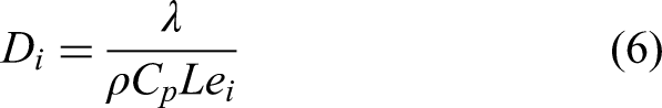
In addition to the mixture-averaged transport model, S3D also features a “LEWIS” transport model where individual species Lewis numbers can be specified. In this method, the thermal conductivity is calculated using the relation proposed by Smooke et al.
44


Two crucial deficiencies associated with the “LEWIS” transport model must be mentioned at this point. First, the power-law expression of equation (4) has been verified only for premixed natural gas flames under stoichiometric and lean conditions.
44
For hydrogen flames, a revision to the form and coefficients of equation (4) may be required. However, this is not attempted in this work, since the aim is to compare the existing state of the “LEWIS” model in S3D with other detailed approaches. Furthermore, a constant value of Prandtl number of
With regard to the boundary conditions, open (inlets, outlets) and closed (walls, symmetry plane) boundaries are treated differently in S3D. For open boundaries, the NSCBC methodology41,45 as previously explained is used to impose boundary conditions. A “non-reflecting” outflow with a relaxation coefficient of
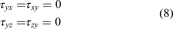
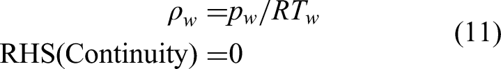
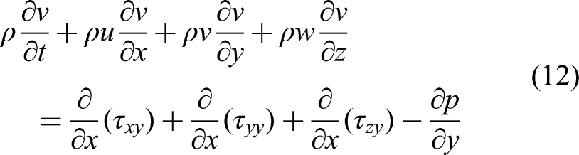
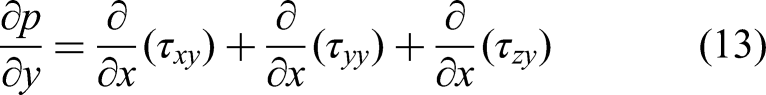
In the following, we detail the implementation of the symmetry plane and the composite wall in S3D, since both of these were newly added to the solver framework. The symmetry plane was modeled as an adiabatic slip wall wherein the wall-normal velocity is zero. Therefore


The specification of the solution vector for a composite wall follows similarly to the implementation for a symmetry plane. In the following, we only highlight the differences between the implementation of a composite wall in relation to the symmetry plane. For velocities, in addition to equation (7), the tangential velocity components and the RHS of the momentum equations in the tangential direction are set to zero. The total internal energy for the adiabatic portion of the wall is computed by solving the energy equation with the normal heat flux set to zero, while for the isothermal portion of the wall it is determined using the wall temperature 
Fluent computational methodology
The incompressible reactive flow solver in ANSYS Fluent v2024 R1 is used for the laminar premixed flame computations reported in this paper. In this framework, variations in density are only due to temperature changes and the pressure is assumed to be spatio-temporally constant. We use the incompressible flow solver since prior works have shown that for propagating flames stabilized at low Mach numbers, the resolution of acoustic waves is not strictly essential for the correct determination of the flame dynamics. At low Mach numbers, the magnitude of pressure and temperature fluctuations imposed by an acoustic wave are weak, and heat release fluctuations caused by an acoustic wave is mainly due to velocity fluctuations and the hydrodynamic processes induced by these oscillations, which are well captured by an incompressible framework.47,48 Furthermore, an incompressible approach precludes the possibility of acoustic resonances in the system and does not demand carefully tailored boundary conditions and input signal amplitude selection to avoid non-linear effects. 47 The validity of the incompressible approach is also asserted by comparison of the FTFs with a fully compressible approach in this paper (see Figure 10).
The thermodynamic properties of the reactive mixture are computed using the “ideal-gas-mixing-law” in Fluent. This framework requires the specification of the species viscosity, thermal conductivity, specific heats, and enthalpies. The species-specific heats and enthalpies are specified as polynomial functions of temperature, while the viscosity and thermal conductivity are computed using the “kinetic-theory” model, which uses the Lennard–Jones characteristic length and energy parameters. 49 The mass diffusion coefficients of each species are also determined using the “kinetic-theory” model, which implements the mixture-averaged transport model approach. The binary diffusion coefficients of each species pair is calculated using the Lennard–Jones characteristic length and energy parameter. The equations involved in the implementation of the mixture-averaged transport model are listed in Table 1. In addition to the mixture-averaged approach, computations are also performed using the unity-Lewis approach, where the species diffusion coefficients are computed by assuming a Lewis number of unity.
With regard to the boundary conditions, a “velocity-inlet” condition is imposed at the inlet which specifies the flow velocity, temperature, and species mass fractions. For the acoustic forcing at the inlet, a time-varying inlet velocity profile is specified using a user-defined function. Isothermal/adiabatic wall boundary conditions are imposed at the top boundary, while a “Symmetry” condition is imposed for the bottom boundary. At the outlet, the “pressure-outlet” condition is imposed which specifies a gauge pressure. The “Finite-Rate” chemistry model is used with a stiff chemistry solver utilizing the “Direct Integration” methodology. The SIMPLE scheme
50
is employed for the pressure–velocity coupling. Under-relaxation factors of
Numerical schemes used for time and space discretization in Fluent.
Results
This section presents the key results of this article, and is organized into two key subsections. The first subsection presents the static and dynamic flame characteristics obtained from the different flow solvers with the mixture-averaged transport model, while the second subsection discusses the impact of the transport models on the hydrogen flame characteristics.
Comparison of flow solvers
First, it is instructive to compare the unstretched laminar flame speed obtained from the various solvers employing the mixture-averaged (MA) transport model. Figure 3 plots the values of the unstretched laminar flame speeds obtained from the 1D computations of hydrogen flames employing different solvers (the tables are given in the Appendix). The operating conditions are chosen in the low equivalence ratio regime where the thermo-diffusive effects are prominent.
17
The reduced version of the San-Diego mechanism designed for hydrogen and ammonia-hydrogen combustion under preheated conditions proposed by Jiang et al.
53
is used for the chemical kinetics description in all solvers employed in this study. First, all solvers predict the unstretched laminar flame speed with a good quantitative accuracy in comparison to Cantera. Second, the influence of Soret diffusion has a noticeable impact on the unstretched laminar flame speed of the hydrogen flames. Indeed, the

Unstretched laminar flame speeds computed for the one-dimensional (1D) premixed hydrogen flame at equivalence ratios of
Figures 4 and 5 depict the flame structure (contours of the heat release rate) for the H

Heat release rate contours of hydrogen flame at an equivalence ratio of
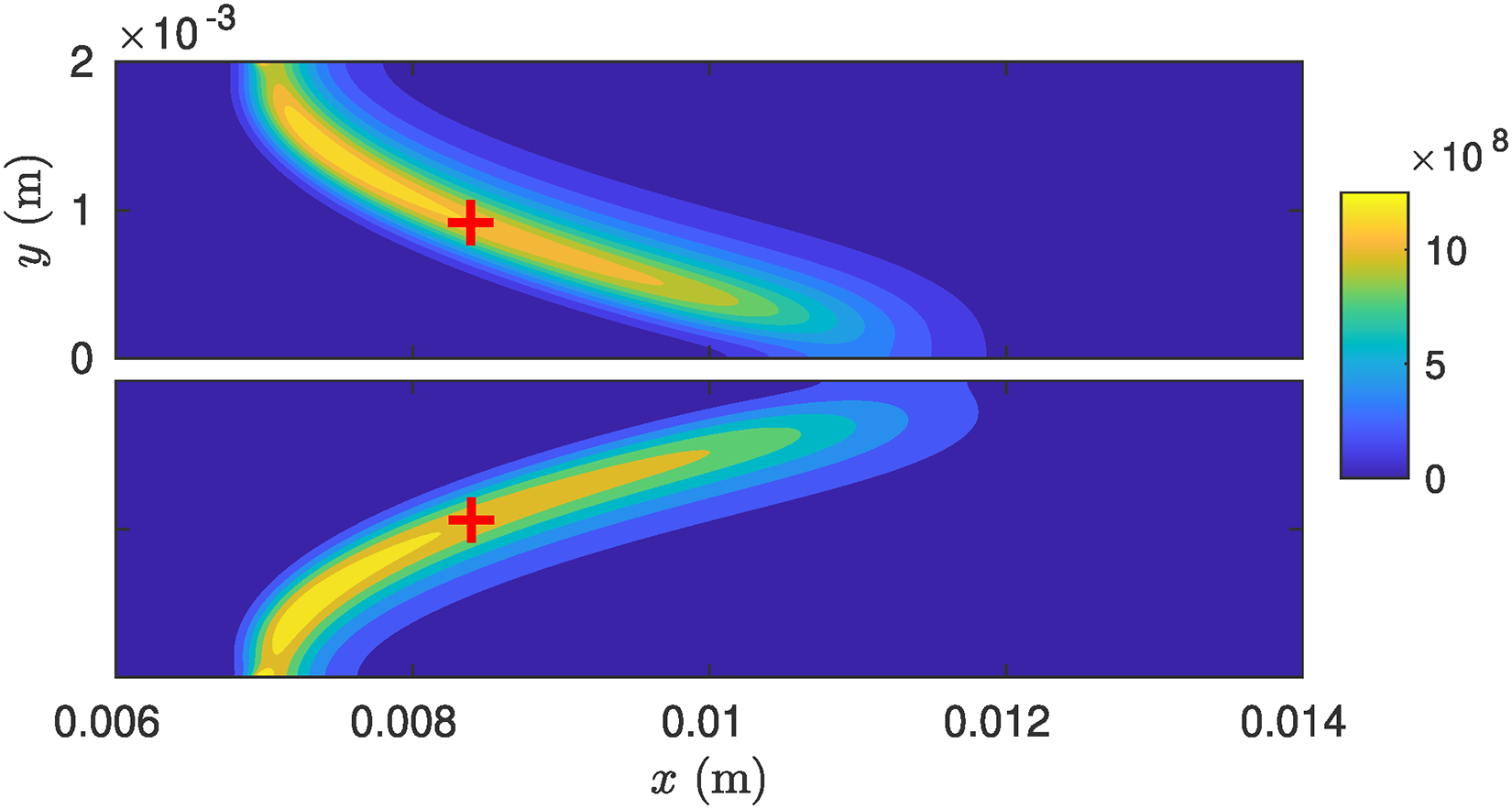
Heat release rate contours of hydrogen flame at an equivalence ratio of
A key parameter that quantifies the flame speed enhancement due to thermo-diffusive effects is the ratio of the global consumption speed (
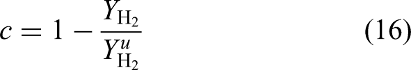
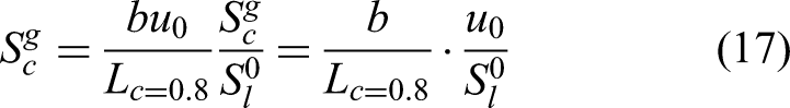
Figure 6 plots the ratio

Comparison of the ratio of the global consumption speed to the unstretched laminar flame speed corresponding to the two-dimensional (2D) slit-stabilized flame obtained with different flow solvers. MA transport model is used in all solvers. MA: mixture-averaged.
Next, the response of the laminar premixed hydrogen flames computed using the different solvers is presented and compared. The flame dynamics are quantified via the heat release rate transfer function (equation (1)), with the reference location for the velocity fluctuations being the inlet of the domain. Two methods are used to compute the FTF. First, by imposing velocity fluctuations at the inlet which are purely harmonic in nature, that is
Alternatively, the imposed time variation of the velocity fluctuations can also take the form of a discrete random binary signal (DRBS), which essentially represents a signal containing a superposition of many frequencies. In this work, a low-pass filtered DRBS signal which takes binary values corresponding to the maximum and minimum velocity fluctuations is used following Huber.
57
The complete impulse response and the FTF can then be obtained with one computation using system identification procedures as explained in detail in Polifke et al.
58
and Polifke.
8
The optimal length of the impulse response is decided by gradually increasing it from
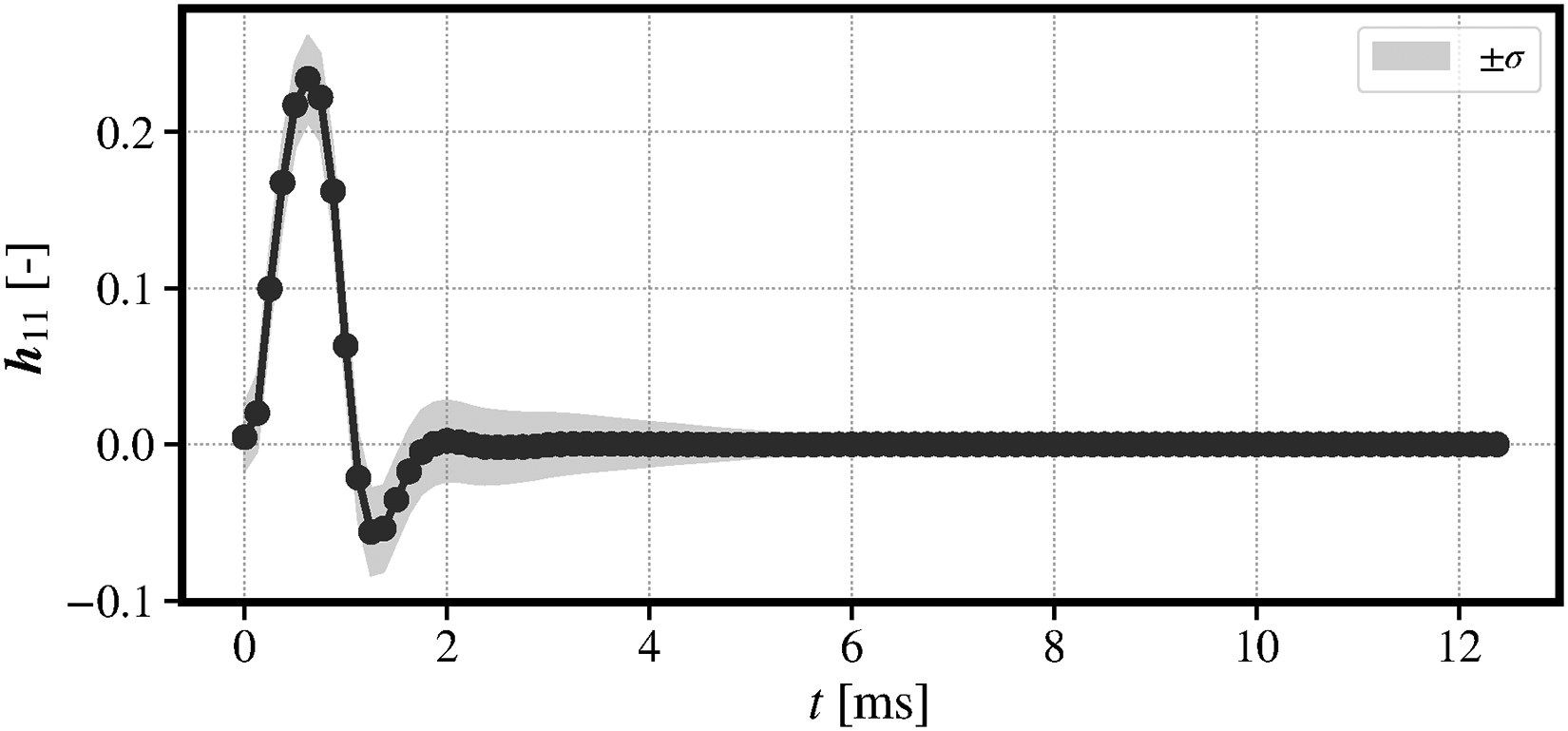
Unit impulse response of the hydrogen flame at an equivalence ratio of
In an open-loop framework, it is advisable to impose non-reflecting boundary conditions at the outlet to prevent possible reflected waves from altering the flame dynamics, and hence the FTF. Reflected waves at the outflow would introduce pressure and velocity perturbations. Since acoustically compact premixed flames are more sensitive to velocity disturbances than to pressure disturbances,
17
and because the reflection delay time (
The quantitative differences in the FTFs obtained from the various solvers and transport models are quantified in terms of the root-mean-square-difference (RMSD) defined as
60

Figure 8 plots the FTFs computed for the hydrogen flames under the conditions considered in this work using the different solvers. The inlet mean velocity is maintained to be thrice the unstretched laminar flame speed obtained from Cantera, and is therefore fixed for a given equivalence ratio across solvers. The FTFs are computed by imposing a time-harmonic signal at multiple discrete frequencies in S3D, and using the DRBS combined with system identification for OpenFOAM, Fluent, and AVBP. To verify the correctness of the implemented system identification techniques to reconstruct the FTF when using the DRBS signal, companion harmonically forced computations were also performed in OpenFOAM (not shown here). For all the equivalence ratios, an excellent match between the two approaches was observed, thus verifying the implemented system identification procedure.
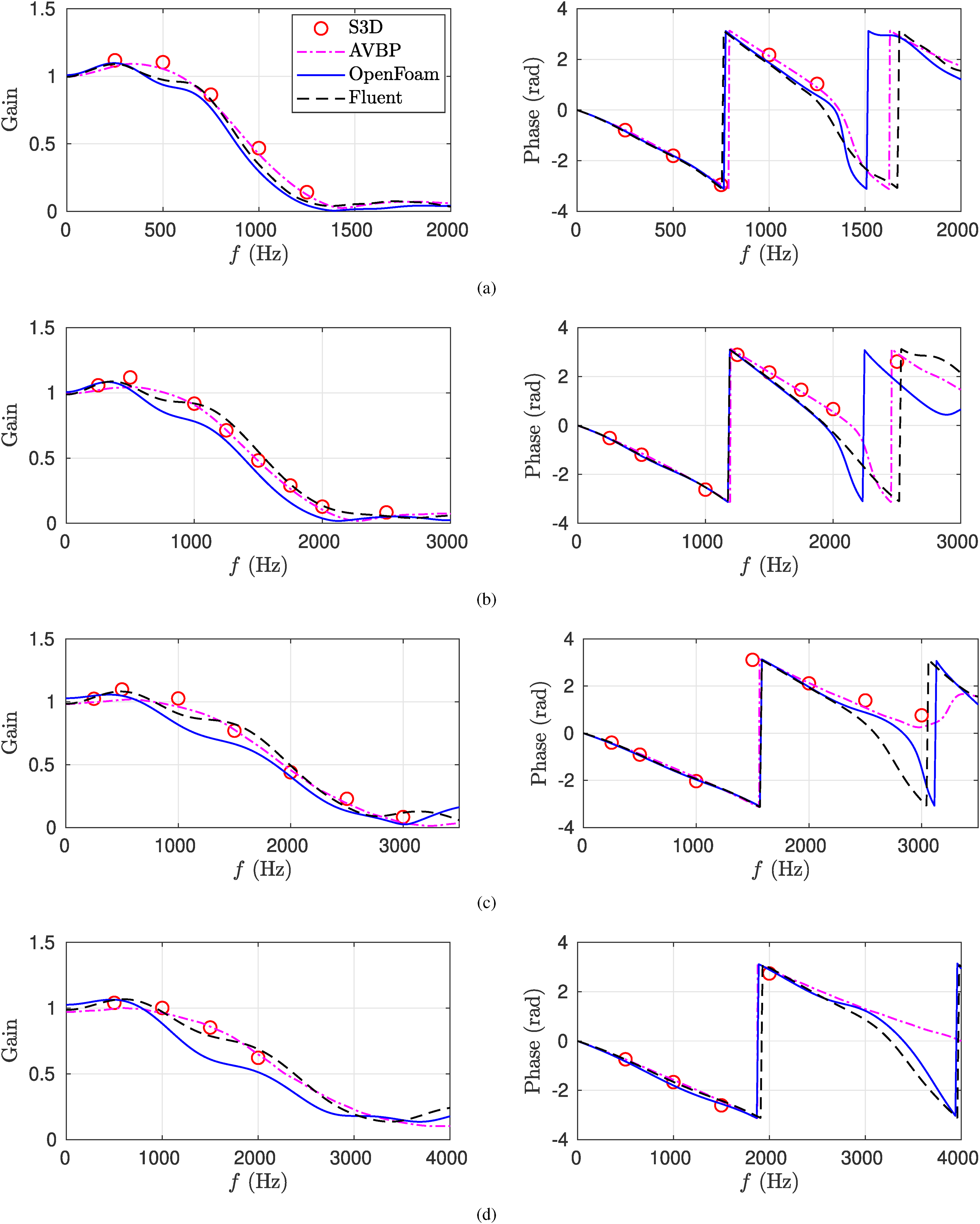
Flame transfer functions of hydrogen flames at equivalence ratios of 0.20 (a), 0.25 (b), 0.30 (c), and 0.35 (d) computed with different solvers. Mean inlet velocities of
Two key observations can be deduced by comparing the FTFs computed with the different solvers in Figure 8. First, the phase of the FTF, which contains the information about the time lag(s) characteristic of the flame, specifically, to the fundamental mechanism that causes the flame response, agrees extremely well across the solvers. Discrepancies, if any, between the solvers are only observed at frequencies where the gain is low. Thus, the essential physics of the physical mechanism(s) resulting in the flame response is captured by all solvers. Second, with regard to the gain, all the solvers still agree well with each other, but noticeable quantitative differences are observed, especially between OpenFOAM and the other solvers. S3D, AVBP, and Fluent agree very closely in gain with each other. Quantitative estimates on the differences between the solvers can be obtained by considering the RMSD metric (equation (20)) tabulated in Table 4. The RMSD of the phase is within
Maximum and minimum values of the RMSD (equation (20)) of the (real, imaginary) part and (gain, phase) of the transfer function compared for different solvers and transport models.
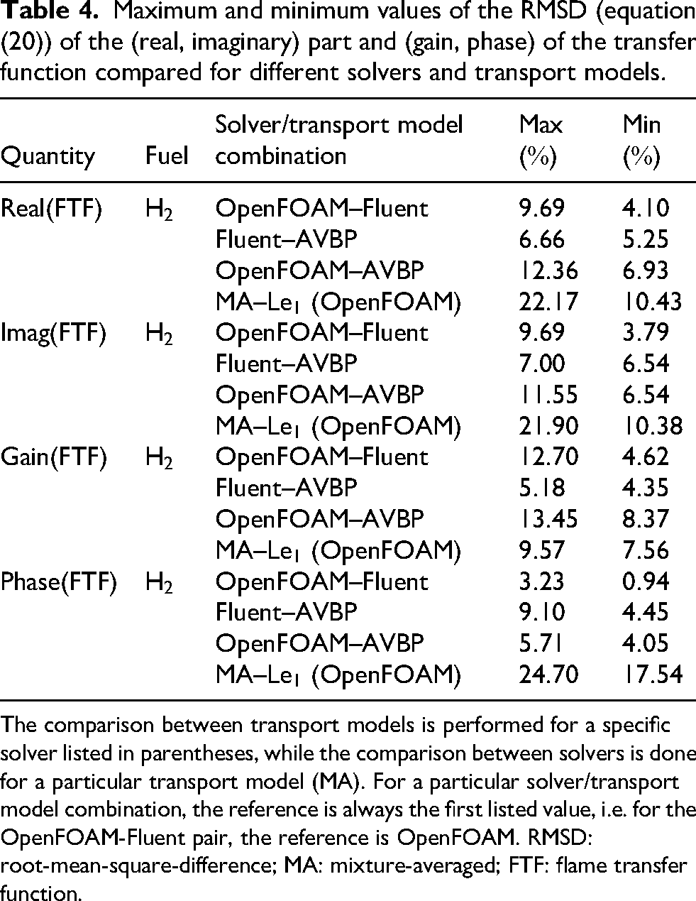
The comparison between transport models is performed for a specific solver listed in parentheses, while the comparison between solvers is done for a particular transport model (MA). For a particular solver/transport model combination, the reference is always the first listed value, i.e. for the OpenFOAM-Fluent pair, the reference is OpenFOAM. RMSD: root-mean-square-difference; MA: mixture-averaged; FTF: flame transfer function.
Next, we examine the influence of variations in the mean inlet velocity profile and the role of pressure fluctuations (compressibility) on the FTFs. To get insight into the former, a plug flow inlet velocity profile and a parabolically varying inlet velocity profile for the identical area-averaged mean velocity are considered. These are shown in Figure 9, where it is to be noted that both profiles have identical area-averaged velocity magnitude. While the parabolic profile is the exact solution of the Navier–Stokes equations in this configuration, the plug flow profile is imposed by default in OpenFOAM and Fluent. To get insight into the role of compressibility, we compute the FTFs of the hydrogen flame in Fluent using the “incompressible-ideal-gas” (weakly compressible) and “ideal-gas” (fully compressible) models. In the weakly compressible approach, density fluctuations are only due to changes in temperature, and the pressure in the domain is assumed to be constant. Figure 10 compares the FTFs obtained using these approaches at two equivalence ratios. In accordance with previous works,47,48 the role of pressure fluctuations on the flame dynamics of the H

Mean velocity profile at a location just upstream of the flame front (6 mm). The velocity profiles are plotted for a plug flow and a parabolic channel flow inlet velocity profile. The area-averaged inlet velocity is identical (
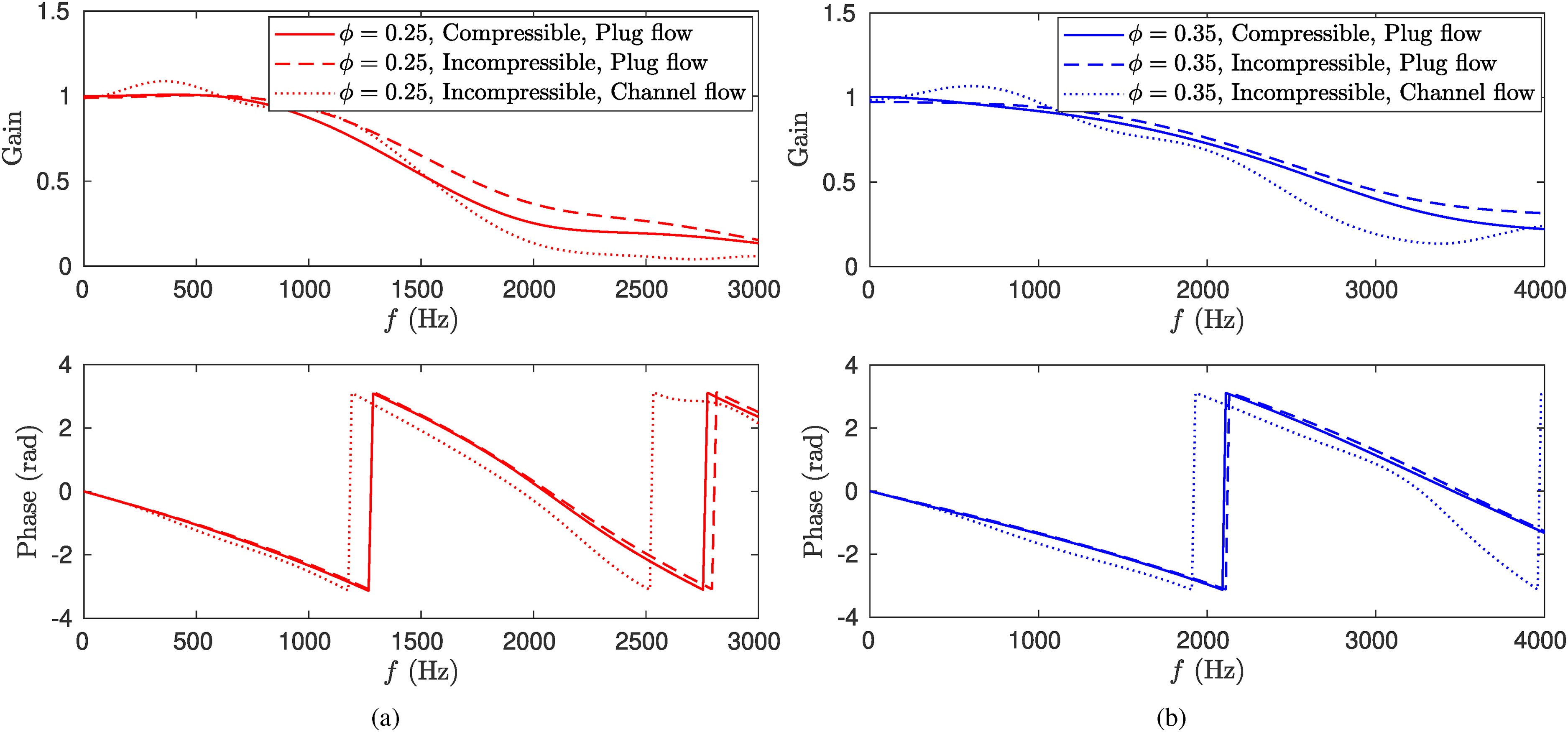
Comparison of the flame transfer functions computed with a fully compressible approach and a weakly compressible approach in Fluent at an equivalence ratio of
The fact that the FTF phase is sensitive to the transverse variation of the velocity profile can be explained by the time-lag characteristic to the flame, which, in this case, is given by the time taken for a flame sheet disturbance to convect from the root to the centroid of the flame with a speed corresponding to the local flow velocity along the flame-tangential direction.
61
This time delay can be mathematically expressed as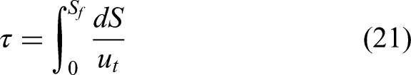
Finally, we conclude this section by summarizing the computational times taken for the FTF calculations using the various solvers and present an analysis for the optimal grid to use in accurately computing the FTFs of the H
Wall-clock time taken to compute the FTF using the various CFD solvers.

The computations are performed for a time of
Furthermore, to determine the “cheapest” setup that yields a good prediction of the FTF, computations of the hydrogen flame dynamics at

FTFs of the hydrogen flame at
Comparison of transport models
In this section, a comparison of the flame dynamics with different transport models is presented. Three transport models are considered: the mixture-averaged transport model (designated as “MA” henceforth), the transport model with specification of individual species Lewis numbers corresponding to the unburnt state of the reactant mixture (designated as “Le
First, it is instructive to compare the unstretched laminar flame speeds for a given solver (S3D) employing different transport models (see Figure 12, values are listed in the Appendix). It is evident that the unity-Lewis approach, due to neglect of the fast molecular diffusion of hydrogen, gives an incorrect estimate of
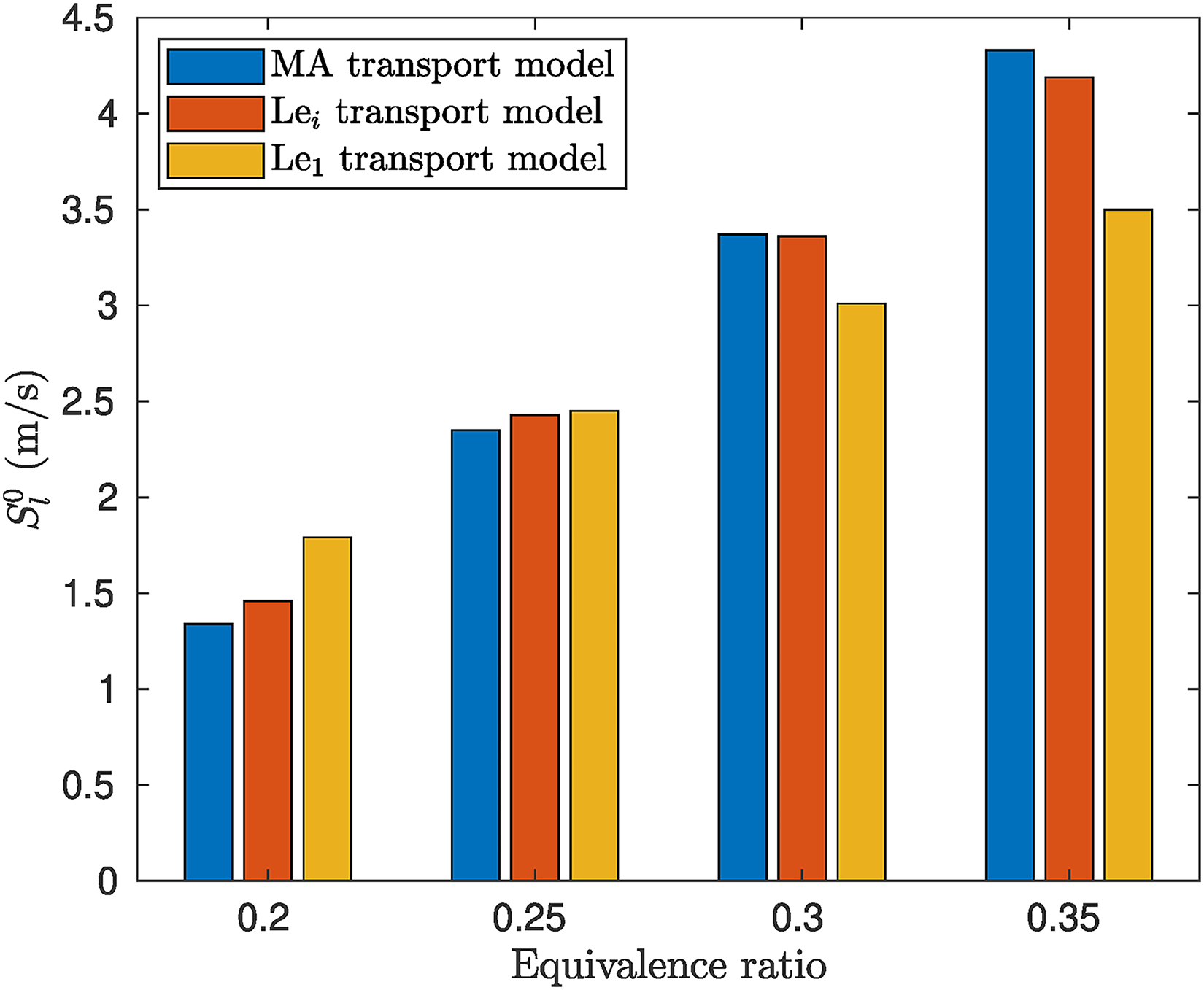
Comparison of the unstretched laminar flame speed obtained in S3D using the MA,
Figures 13 and 14 depict the mean flame structure in terms of the normalized heat release rate (

Normalized heat release rate contours of hydrogen flame at an equivalence ratio of
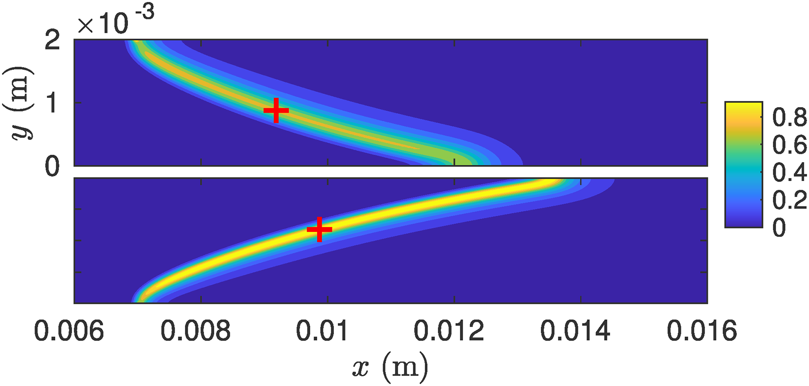
Normalized heat release rate contours of hydrogen flame at an equivalence ratio of
In summary, when using a unity-Lewis approach to compute the flame structure, drastic differences may be observed, first due to neglect of thermo-diffusive effects resulting in an incorrect heat release distribution, and second due to the different

Comparison of the ratio of the global consumption speed to the unstretched laminar flame speed computed from the S3D solver with different transport models.
Figure 16 compares the FTFs obtained for hydrogen flames using the mixture-averaged and the unity-Lewis number transport model in OpenFOAM. Noticeable differences not only in the gain, but also in the phase of the transfer functions are observed. The reason for this can be easily deduced from Figure 12. For a given solver, the unstretched laminar flame speed computed with a unity-Lewis transport model is different from the corresponding mixture-averaged flame speed. For a fixed flow velocity, this results in a different flame length, which shifts the centroid of the heat release distribution, resulting in different time delays (see e.g. Figures 13 and 14). Furthermore, with regard to the gain, the unity-Lewis transport model does not capture the thermo-diffusive effects. Therefore, it does not capture the influence of flame speed fluctuations on the heat release dynamics. In addition, due to the different unstretched laminar flame speed and the global consumption speed between the unity-Lewis and mixture-averaged approaches, the flame shapes are different resulting in different area responses. It is, thus, no surprise that the gain of the FTF changes when using mixture-averaged and unity-Lewis transport models. In terms of the quantitative RMSD metric, the phase of the FTFs shows differences as high as

Flame transfer functions of hydrogen flames at equivalence ratios of
Finally, we assess the effectiveness of the Le

Flame transfer functions of H
In summary, the results of this section demonstrate that the proper selection of transport model is crucial in the computation of FTFs of hydrogen flames. First, using the unity-Lewis transport model for hydrogen can result in inconsistent results due to the inability of this model in capturing the thermo-diffusive effects. Indeed, for the current operating conditions, the quantitative deviations in the FTF of the unity-Lewis approach in relation to the more detailed mixture-averaged transport model were about
Conclusions
The advent of carbon-free fuels, with different reactivity and transport properties in relation to conventional fuels, for sustainable power production calls for robust computational tools to accurately predict the combustion characteristics of these fuels. Therefore, it is important to compare existing CFD solvers from the standpoint of static and dynamic flame characteristics of these carbon-free fuels. In this paper, computations of laminar premixed flame shapes and dynamics (response to acoustic perturbations) with four CFD solvers (ANSYS Fluent, OpenFOAM, AVBP, and S3D) were performed and compared. It was first shown that, despite using the identical chemical kinetic mechanism and similar transport models, quantitative differences up to
The second key contribution of this work is the observation that the incorporation of non-unity-Lewis numbers of hydrogen is highly essential in capturing the correct flame dynamics. Using a unity-Lewis approach gives inaccurate estimates of the unstretched laminar flame speeds, and does not capture key processes characteristic of hydrogen flames such as flame speed enhancement due to stretch, non-uniform heat release distributions along the flame sheet and tip-opening. Furthermore, assuming all species Lewis numbers to unity results in errors as high as
Footnotes
Funding
The authors disclosed receipt of the following financial support for the research, authorship, and/or publication of this article: Harish S. Gopalakrishnan was funded by the Swiss National Science Foundation (SNSF) under the project ADONIS (Ammonia hydrogen combustion in micro gas turbines) with the grant number 206244.
Declaration of conflicting interests
The authors declare no potential conflicts of interest with respect to research, authorship, and publication of this article.