The Influence of Occupancy Change on Hotel Market Equilibrium

Abstract

Supply and demand imbalances in hotel markets are known to cause short-term growth or declines in rate and are largely (but inefficiently) self-correcting over the long term. However, looking at aggregated monthly supply and demand shifts for a market overlooks the dramatic shifts that typically occur daily within a market. Building on natural occupancy rate theory and using daily performance over a 5-year period for the Seattle Metropolitan Statistical Area (MSA) and submarkets, this study shows that examining daily occupancy patterns provides important insights into average rate growth. Furthermore, the analysis shows that the real average rate growth is a function of not only absolute occupancy levels relative to the market’s natural occupancy rate but also relative changes in occupancy, and that change in occupancy moderates the relationship between occupancy and average rate growth. In addition, submarkets within the MSA have significantly different attributes, including different natural occupancy levels and different responses to changes in occupancy. Implications for hotel investors, managers, and policy planners are then presented.

Keywords

hotel market equilibrium natural occupancy rate

Introduction

Hotels are known to operate in an environment of both short- and long-term demand/supply cycles (Corgel, 2005). On a long-term basis, supply adjusts to changing levels of demand, but the adjustment is inefficient because of the inflexibility of short-term supply (Chen & Chang, 2012). The fixed and perishable nature of room inventory coupled with widely fluctuating demand patterns compel hotels to continuously adjust their prices and their sales and marketing tactics (Kimes, 1989), making the process of managing revenues more complex (Erdem & Jiang, 2016; Kimes, 2015). Understanding market dynamics is critical not only for investors making decisions about where to build new hotels (deRoos, 1999) but also for managers and revenue managers tasked with optimizing revenues and managing inventory for their properties (Gallagher & Corgel, 2018).

Predicting and understanding average rate growth is thus important to investors interested in obtaining returns on their investment, developers assessing new opportunities, and hotel managers setting their pricing strategies and managing their inventory. Managing and optimizing revenues is a much more complicated proposition than when hotel prices were advertised on roadside signs and pricing tools consisted of a ladder and a paintbrush. Revenue management has become a highly structured business process (Buckhiester, 2011a) and has evolved from a tactical inventory management approach to a strategic marketing approach (Kimes, 2015). Stakeholders need to understand the factors that contribute to hotel pricing and the impact that hotel pricing dynamics have on profitability levels for both the individual hotel and the collective market, as overestimating or underestimating future revenue growth can lead to the misidentification of development opportunities (deRoos, 1999).

One of the most difficult factors to incorporate into projecting average rates is the level of market disequilibrium, or the balance between demand and supply (Arenoe et al., 2015). Hotels raise prices to maximize revenue when demand levels are high and reduce prices to fill excess inventory when demand levels are low (Chen & Chiu, 2014). The absence of long-term contractual rates that preclude short-term price manipulation (lease friction) enables hotels to respond in real time to changes in demand, making hotels particularly interesting for studying how real estate asset markets respond to short-term fluctuations in local market forces (Corgel, 2005).

The studies by deRoos (1999), Corgel (2005), and Gallagher and Corgel (2018) have framed the hotel equilibrium theory, which posits that hotel markets have natural occupancy rates at which real average rates remain stable, increasing at the rate of expense inflation. Occupancy levels exceeding this equilibrium rate contribute to increased rate growth, and occupancies below equilibrium contribute to below-inflationary rate growth. This concept of natural occupancy rates and market equilibrium has been firmly established using nationwide or metropolitan-wide monthly occupancy and average daily rate (ADR) observations.

Past studies differ on whether current occupancy levels or prior year occupancy levels are better predictors, leading to some uncertainty on the generalizability of the findings. Furthermore, to date, no research has been published evaluating the factors that influence average rate changes daily, as they truly occur and consistent with how rates are forecasted and managed. Interday variations between occupancy and ADR can be dramatic even if monthly or annual trends are static, and a 70% occupancy month may have dramatically different average rate trends depending on whether occupancy is 70% every day or whether 70% is the simple average of a wide range of daily occupancy levels. Now that the hotel equilibrium theory has been established, it behooves researchers to study markets on a granular level.

In addition to uncertainty over the most appropriate predictor variables, past studies of hotel market equilibrium have explained only a small proportion of average rate variance. The seminal study by deRoos reported that R² values rarely exceed .15, with .10 considered to be a good fit (deRoos, 1999). Gallagher and Corgel’s recent study found R² coefficients of .18 to .20 for the top 60 markets, with individual markets achieving coefficients ranging from .18 to .53 (Gallagher & Corgel, 2018). These low levels and wide ranges of explanatory power indicate that other factors should be explored to try and better explain the forces that drive average rate growth in hotel markets.

The purpose of this study is to expand on the established theory of hotel market equilibrium using data from a single metropolitan market. The first objective of the study is to establish whether prior year occupancy levels (Gallagher & Corgel, 2018) or current year occupancy levels (deRoos, 1999) are more appropriate predictors of average rate growth and whether using daily occupancy observations provides additional reliability compared with monthly observations. Second, this study explores whether the simple linear regression methodology used in past studies provides the best tool for predicting average rate growth or whether additional factors or nonlinearity may be observed by focusing on a more robust data set involving a single metropolitan market. For this study, the Seattle Metropolitan Statistical Area (MSA) was selected as it represents a relatively self-contained study area with little overlap between adjoining regions and has distinctive submarkets operating within the MSA.

This study contributes to the literature by showing that current occupancy levels are better predictors of average rate growth than lag-year monthly occupancy levels. Furthermore, this study shows that average rate growth is influenced by the relative change in occupancy to a greater degree than the absolute occupancy level. Finally, the relationship between occupancy levels and average rate growth is shown to be moderated by the change in occupancy such that declining occupancy levels predict lower average rate growth or even declines in average rate even if occupancy levels are high.

The remainder of this article is organized as follows: The “Literature Review” contains an overview of relevant studies and findings conducted to date. The “Data and Results” section presents longitudinal occupancy and average rate data for the Seattle MSA and evaluates the relative reliability of the predictor variables. From the initial observations, a conceptual model is presented and tested showing changes in occupancy as a moderating variable. The augmented regression formula developed from the conceptual model is then applied to three submarkets within the Seattle MSA to determine whether the relationships are consistent across different regions within the market. Finally, in section “Implications,” implications for hotel investors, developers, and managers are discussed.

Literature Review

Hotel markets are known to be cyclical, with demand patterns closely following changes in gross domestic product (GDP) with supply and investment cycles moving in long-term patterns that have little connection to short-term macroeconomic fluctuations (Wheaton & Rossoff, 1998). The combination of these two patterns results in overall hotel industry cycles that are characterized by long periods of up-cycles and shorter down-cycles with a complete cycle typically occurring every 7 to 10 years (Kalcevic, 2018). The natural progression of recent cycles has often been disrupted or accelerated by external shocks. Recent cycles have corresponded roughly to presidential administrations and include the Clinton cycle from 1991 through 2002 (9 years up and 2 years down), the Bush cycle from 2002 through 2009 (5 years up and 2 years down), and the Obama/Trump cycle from 2009 to the present (9 years up through mid-2019). The existence of these cycles was first identified by Wheaton and Rossoff in 1998, and their predictability and impacts on hotel performance have been extensively studied (Corgel, 2005; Kalcevic, 2018).

The concept of market equilibrium and its impact on consumer pricing decisions in hedonic pricing models was first explored by Rosen (1974). Although this concept was developed to explain product pricing in an environment of equal-value attributes (i.e., consumer income levels are not assumed to influence their demand characteristics or willingness to pay), the short- and long-term equilibrium functions are highly applicable to the hotel business as demand can change in the short term but supply cannot. Rosen’s hedonic pricing model has been utilized in the lodging sector to evaluate pricing differentials between lodging properties based on location, such as the impact of airport proximity (Corgel & deRoos, 1993; Lee & Jang, 2011) or Central Business District proximity (Lee & Jang, 2012a; Shoval, 2006), highlighting the importance of evaluating submarkets within an MSA rather than simply studying an MSA as a single market.

Unlike other real estate classes, hotels have a different perspective on the cost of short-term vacancy. Research by Wheaton and Rossoff (1998) identified that hotels have strategic incentives to make inventory available for demand segments that have short-term booking cycles, as these segments typically pay premium rates. For property types that have long-term leases, discounting rates to avoid leaving space empty can negatively affect profitability over several years, so overreacting to short-term vacancy has long-term consequences. For hotels, the lease terms are measured in days, not years, so allowing a room to remain vacant for a single night represents a lost opportunity. Thus, there exists an optimal level of vacancy that is unique to the hotel business up until the last minute—booking rooms too early makes them unavailable for the less price-sensitive customers, but not booking them at all represents an opportunity cost with no strategic benefits. This incentive for hotel managers to commit rooms incrementally without letting them sit empty has contributed to the creation of an entire industry of revenue managers who monitor and manipulate hotel rates on a real-time basis and to a degree that could not have been imagined 20 years ago.

deRoos (1999) and Corgel (2005) expanded on Wheaton and Rossoff’s findings and created a framework called hotel equilibrium theory. This theory builds on the concept that natural occupancy rates exist at which real hotel ADR growth is neutral. When markets perform above the natural occupancy rate, ADR growth is positive in the short term, and additional development is stimulated in the long term to compensate for or absorb the higher levels of profitability. Similarly, when occupancies are below the natural occupancy rate, real ADR growth is negative and additional development is discouraged. deRoos estimated the natural occupancy level on a nationwide basis to be 62.9%, with individual markets showing natural occupancy levels ranging from 56.4% to 75.9%. Gallagher and Corgel (2018) subsequently identified that natural occupancy rates are time varying and regime varying and that the natural occupancy rates are higher for higher priced hotels. Their research, which included monthly occupancy and ADR observations from 1988 through 2017, suggested that natural occupancy rates range from 60% to 77% depending on the city, lodging subgroup, and whether the market is in a normal or recessionary environment.

Market equilibrium has been adopted to different degrees and with varying levels of success by researchers. Chen and Chiu (2014) showed that market disequilibrium has a significant impact on hotel pricing in Taiwan and that incorporating a market equilibrium variable into a hedonic pricing model improved the predictive ability of the model using monthly observations of tourist hotels from 1996 to 2008. Price instability resulting from disequilibrium has been shown by some researchers to improve profitability levels (Oi, 1961), but Tisdell (1963) and Chen and Chang (2012) found that instability/disequilibrium had a negative impact on hotel profitability. Lee and Jang (2012a) used fundamental price theory to determine optimal capacity levels of the U.S. lodging industry, concluding that the optimal ratio of supply growth to demand growth is 1.535:1, equating to an equilibrium occupancy level of 65.1% using monthly U.S. data from 1987 through 2010.

Although research has been invaluable in developing hotel market equilibrium theory, the level of noise in the data indicates that there is still work to be done to uncover factors contributing to ADR growth rate levels. Wheaton and Rossoff (1998) indicated that significant noise exists in their original model, and the predictive power of Gallagher and Corgel’s time-varying models admittedly varied, with R² coefficients ranging from .18 to .52 (Gallagher & Corgel, 2018). Furthermore, natural occupancy rates vary over time as technology, labor costs, and other inputs change, requiring periodic evaluations to determine whether conclusions based on data from past studies are still reliable (Gallagher & Corgel, 2018).

Occupancy and rate levels fluctuate daily depending on the composition of demand and demand factors. As hotel room inventories are perishable commodities, hotel revenue management is a daily task, and the hotel’s performance on a weekday has little bearing on the rate strategies for the coming weekend. Similarly, one month’s high-occupancy levels do not provide any relief from the requirement to fill rooms in the subsequent month(s).

Thus, two cities or submarkets could have identical monthly or annual occupancy levels but dramatically different interday patterns and consequently different ADR growth levels because of the number of high- or low-occupancy days that they experience throughout the period. However, there is no known literature investigating the effect of daily occupancy patterns on hotel market compression levels.

This study utilizes daily occupancy and ADR patterns from 2014 through 2018 in the Seattle metropolitan area using data provided by Smith Travel Research (STR). Seattle was chosen for this analysis because it exhibits the characteristics of a typical metropolitan market in that the CBD was observed to have different occupancy/rate patterns from the suburban and airport submarkets. Seattle was also determined to be an interesting market to study because it has benefited from strong occupancy levels over an extended period of time, resulting in above-equilibrium rate growth, and has not experienced a recession or regime change during the study period. If a recession or regime change had occurred, bifurcation of the data would be required, or additional noise would be introduced into the data. This study expands on the established hotel market equilibrium theory by investigating whether hotel market dynamics operate on a granular level, with rates adjusting daily and patterns varying between submarkets within a metropolitan area.

Data and Results

Daily occupancy and average rate data for the Seattle MSA and three submarkets, Seattle (CBD), the Eastside (including Bellevue, Redmond, Kirkland, Bothell, and Woodinville), and the SeaTac Airport, were obtained from STR. For the monthly analysis, data were obtained from 2012 through 2018 (84 observations for each market), and for the daily analysis, data were obtained from 2014 through 2018 (1,826 observations for each market).

Seattle Market Overview

During the observation period, Seattle is representative of a healthy business environment and a strong hotel operating market. Over at least the past 7 years, the Seattle MSA has benefited from enviable hotel demand growth rates according to data provided by STR. Demand has grown at a compounded annual rate of 2.9% that was only partially offset by an annual supply growth of 1.9%, resulting in occupancy levels increasing from 69.7% in 2012 to 76.1% in 2017, before easing back to 74.7% in 2018. The average rate growth averaged 4.5% per year, and this combined with the increases in occupancy produced revenue per available room (RevPAR) growth of 5.5% per annum, which is well in excess of the local consumer price index (CPI) growth of 2.0%.

However, developer interest in building new hotels has increased, with the guestroom supply increasing by nearly 8,500 rooms (18.6%) over a 6-year period, from 45,563 rooms in January 2012 to 54,039 in December 2018. Projects in the development or planning stages also added another 9,000 rooms in just 3 years. Chart 1 presents the summary performance of the Seattle MSA, utilizing data obtained from STR.

Chart 1.

Seattle MSA Consolidated Annual Performance.

The market-wide data suggest that the Seattle MSA remains healthy in terms of demand and rate growth, with ADR continuing to increase above the rate of inflation, despite supply growth of 5.1% in 2018. Looking solely at these data, it would be tempting for developers to declare the Seattle MSA to be a strong hotel market capable of absorbing significantly more hotels and for existing hotels to forecast above-inflationary average rate growth to continue unabated. This view is where annual aggregate data can obscure significant disparities that may be occurring on a daily or subregional basis, and daily disaggregated data may provide greater insights into the overall health of the market.

Current Versus Lag-Year Occupancy as Predictor of Average Rate Growth

Initial models for estimating natural occupancy rates were developed by deRoos (1999) based upon the work of Wheaton and Rossoff (1998). The model employed by deRoos assumed that average rate growth was determined by CPI growth and occupancy level, $Δ A D R = b_{0} + b_{1} (Δ C P I) + b_{2} (O C C)$ . The natural occupancy rate is determined as the point at which ΔADR is 0, which is calculated as −(b₀ / b₂).

Gallagher and Corgel (2018) expanded upon the deRoos model based on the rental adjustment model developed by Rosen and Smith (1983) with modifications to account for CPI, as $Δ R A D R_{t} = β_{1} (O_{a t - 1} - O_{n} - φ s_{t} - ζ R_{t}) + ε_{t}$ , where $R A D R_{t}$ represents the change in real ADR at time t $(\frac{R A D R_{t} - R A D R_{t - 1}}{R A D R_{t - 1}})$ , O_at−1 represents the lag-period occupancy level, and O_n represents the natural occupancy level at which real ADR growth is neutral. In addition, S_t is an added Markov switching variable that is coded with a value of 0 when the market is operating under normal baseline conditions and a value of 1 when the market is operating under an alternate natural occupancy state, and R_t is a dummy variable added to indicate a recessionary environment.

Under normal state conditions, the S_t and R_t variables are coded to 0 and are eliminated from the equation, and if current occupancy levels are equal to the natural occupancy rate, then the entire right side of the equation collapses and real rate growth equals the error term. In adapting this model to study the Seattle MSA, the authors considered that no recessions or regime changes have occurred during the study period, causing the S_t and R_t variables to have no effect and enabling a clearer picture of β₁ to emerge during normal market conditions. The comparison between the deRoos and the Gallagher and Corgel models thus comes down to a question of whether current year occupancies or prior year occupancies are better predictors of average rate growth.

Table 1 presents an assessment of real average rate growth experienced in the Seattle MSA from 2014 to 2018 using the two prevailing methodologies:

Table 1.

Natural Occupancy Level Predictions Using Prior Year and Current Year Occupancy (Monthly Observations).

Independent Variables	Model 1A			Model 1B
	Prior Year Occupancy			Current Year Occupancy
	R ²	SEE	p value	R ²	SEE	p value
	.10	0.04	.01	.18	0.03	.00
Predictors	Predictor Statistics			Predictor Statistics
Predictors	B	T	p value	B	T	p value
Constant	−0.06	−1.82	.07	−0.09	−3.00	.00
Prior year occupancy	0.11	2.77	.01
Current occupancy				0.16	3.95	.00
Implied equilibrium occupancy level	48.7%			57.2%

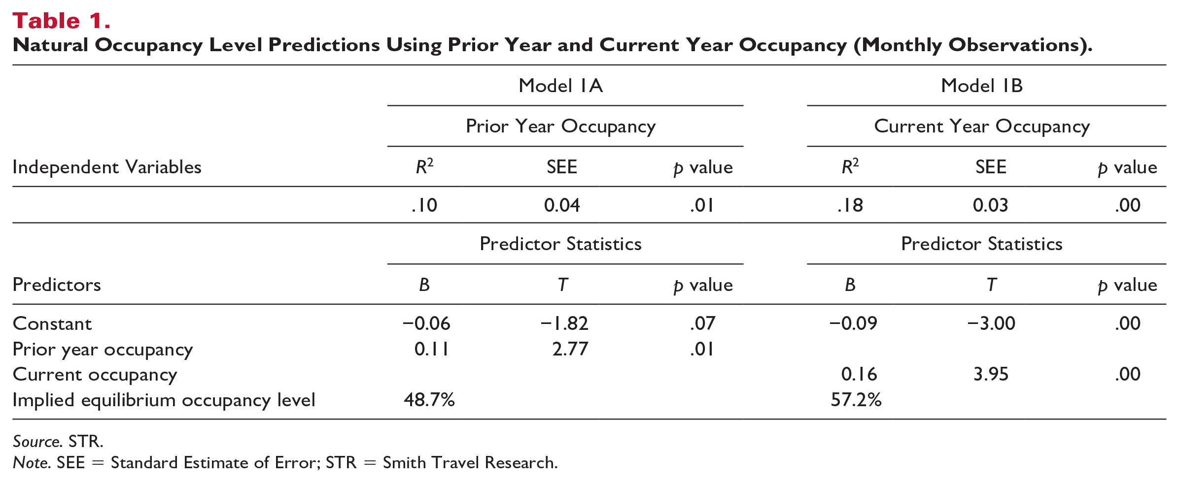
Source. STR.

Note. SEE = Standard Estimate of Error; STR = Smith Travel Research.

Table 1 suggests that current year occupancy levels are more appropriate predictors of average rate growth than prior year occupancies, with an R² of .18 compared with R² = .10. The implied natural occupancy level for the Seattle MSA using monthly observations over this time period would be 57.2%, suggesting that real ADR growth would be positive when occupancies exceed this level with rates increasing by .16% for every one-point increase in occupancy. The relatively low predictive power of this equation is consistent with the admonition by deRoos that reliability coefficients rarely exceed .15 and that levels of .10 or higher should be considered a good fit (deRoos, 1999).

Assessing Daily Occupancy Patterns

To determine whether daily occupancy observations provide greater reliability than monthly data, the authors analyzed daily occupancy and average rate data provided by STR. Seasonal and weekly travel patterns instill a certain level of inefficiency in any hotel market (Lee & Jang, 2012a), as hotel supply should be adequate to capture demand during peak travel periods but not so great that an excessive number of rooms sit empty during nonpeak periods. For this study, year-to-year comparisons were made based on day-of-week (Saturday vs. Saturday) observations rather than calendar dates (January 1 to January 1). This method is necessary to avoid the noise created by comparing different weekdays. No adjustment was made for holidays (e.g., Christmas falling on a Monday in 2017 but a Tuesday in 2018) even though the variances were significant, but it is worth noting that this level of noise is inherent when using daily observations.

The daily data show that although the annual occupancy rates for the MSA ranged from 69.7% to 76.1%, the daily observations varied much more dramatically from 33.6% to 98.3% (Graph 1). Closer inspection reveals that weekday periods throughout much of the year are the strongest, with Tuesday and Wednesday occupancy levels regularly exceeding 80%. Weekend occupancies are more variable, with summer weekends operating at very high occupancy levels and weekends in the winter months registering the lowest occupancy levels throughout the year. These patterns are consistent with a market that has a strong commercial base coupled with seasonal leisure visitation.

Graph 1.

Seattle MSA Occupancy Trends: Daily Observations.

Real changes in average rates were then assessed over the range of occupancy observations, as summarized in Table 2.

Table 2.

Real ADR Growth by Occupancy Cohort: Seattle MSA (2014–2018).

Occupancy Cohort (%)	N	Real ADR Growth (%)	SE (%)
90+	252	5.04	0.37
85–90	215	4.26	0.43
80–85	198	3.07	0.44
75–80	215	1.28	0.39
70–75	170	0.02	0.46
65–70	124	−0.15	0.60
60–65	69	−0.48	0.72
55–60	73	−1.52	0.79
50–55	53	−2.64	0.82
<50	84	−2.52	0.68
Sum/Avg	1,453	1.76	0.17

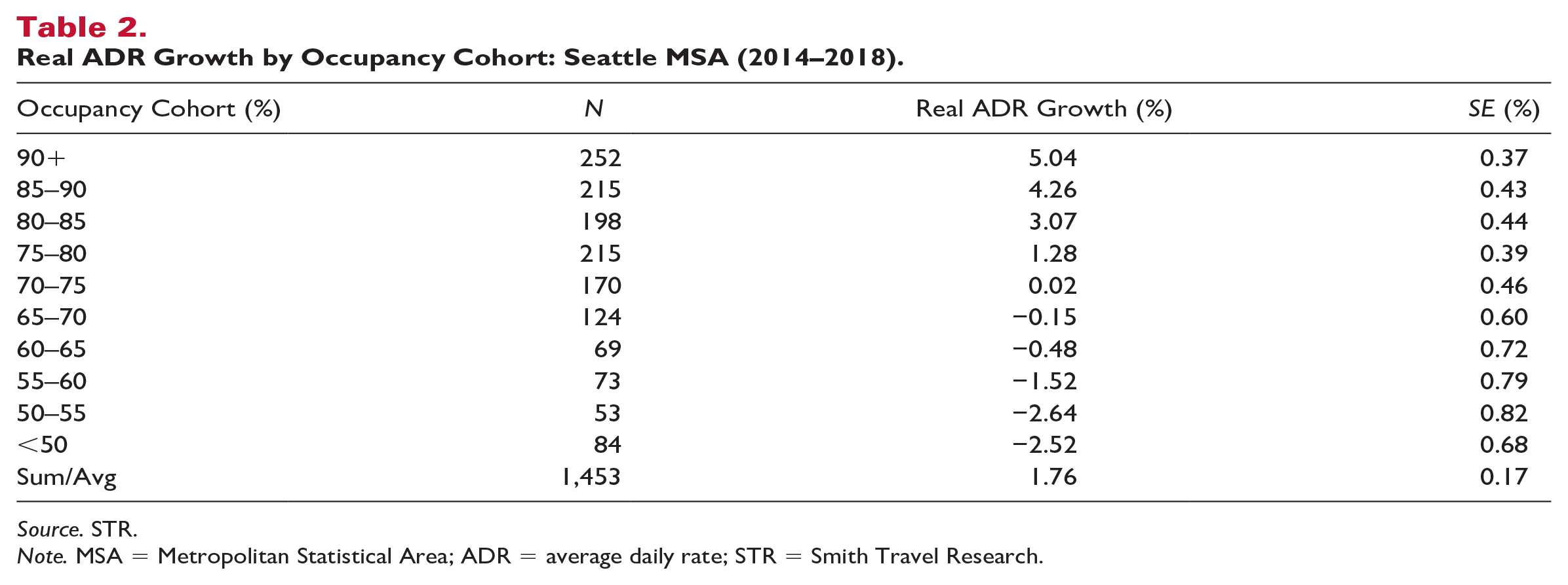
Source. STR.

Note. MSA = Metropolitan Statistical Area; ADR = average daily rate; STR = Smith Travel Research.

Table 2 illustrates the market’s ability to drive higher average rate growth during periods of high occupancy and suggests that the natural occupancy rate for the Seattle MSA during this time period is between 65% and 75% rather than the 57.2% level provided by Model 1B in Table 1. This indicates that daily occupancy observations provide a different picture than monthly observations, and the study of daily observations provides additional insights. The degree of variation in the average rate changes, as expressed by the standard errors of the estimates, indicating that greater variability is experienced at lower levels of occupancy. Chart 2 illustrates the variation in average rate change and the variability of that change (as represented by the standard error bars).

Chart 2.

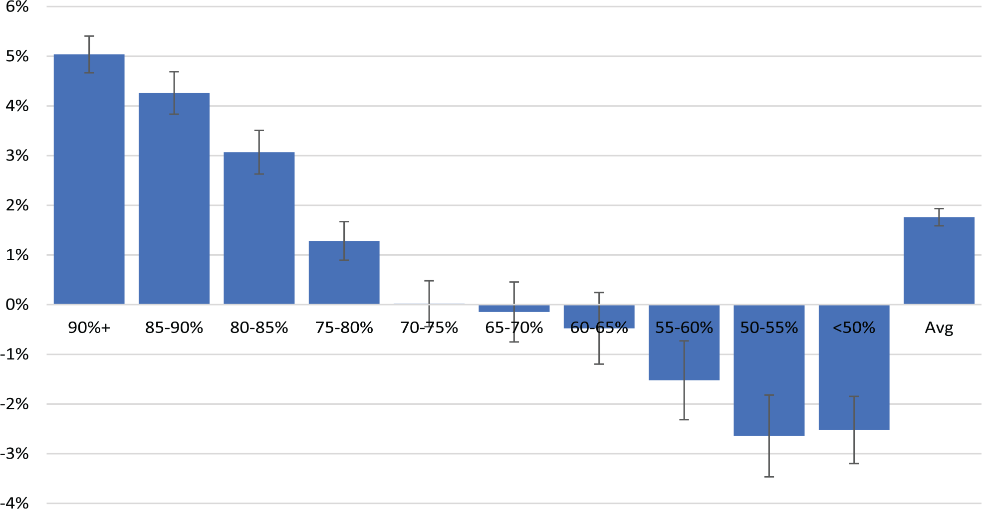
Seattle MSA Real ADR Growth (2014–2018) by Occupancy Cohort.

The results provide support for past studies suggesting a natural occupancy rate relationship between occupancy levels and ADR growth, but the results question whether the relationship is linear, with rate growth accelerating as available supply levels tighten. These data also present more insights into the natural occupancy rate as occurring within the range of 65% to 75% occupancy, where real ADR growth transitions from being negative to being positive. However, the significant levels of variation show that the levels of ADR growth vary dramatically even within each occupancy cohort, providing some insights into the low R² coefficients found in Table 1 and in past studies.

As discussed, the variation in daily occupancy levels is significantly greater than the variation in monthly or annual data, implying greater errors using simple linear regression and lower R² values. Table 3 presents the results of this application of the simple regression.

Table 3.

Regressing Average Rate Growth on Daily Occupancies.

	Model 2
	Current Year Occupancy
Independent Variables	R ²	SEE	p value
	.12	0.07	.00
Predictors	Predictor Statistics
Predictors	B	T	p value
Constant	−0.12	−12.07	.00
Current occupancy	0.18	14.29	.00
Implied equilibrium occupancy level	65.7%

Note. SEE = Standard Estimate of Error.

The results from Model 2 differ significantly from the conclusions reached by evaluating monthly observations, with an implied equilibrium occupancy level of 65.7% and a slightly higher average rate growth of 0.18% for each one-point increase in occupancy. The R² value of .12 (p < .001) is lower than the R² using monthly observations but is still significant and is expected, given the greater variation in daily occupancy observations compared with monthly observations. The dispersion of observations daily makes the reliability of predictors more challenging but also provides additional insights into the factors that drive average rate growth and market equilibrium.

Utility of the Single-Predictor Model

To assess whether the single-predictor regression model is most appropriate, the authors evaluated daily changes in the real average rate over the spectrum of observed occupancy levels. If the single-predictor model holds, then the average rate growth is positive when the occupancy is greater than the natural occupancy rate of 65.9% and negative when below 65.9%. Graph 2 presents a plot of the observations when daily average rate growth is regressed on occupancy levels, with the linear prediction line illustrated.

Graph 2.

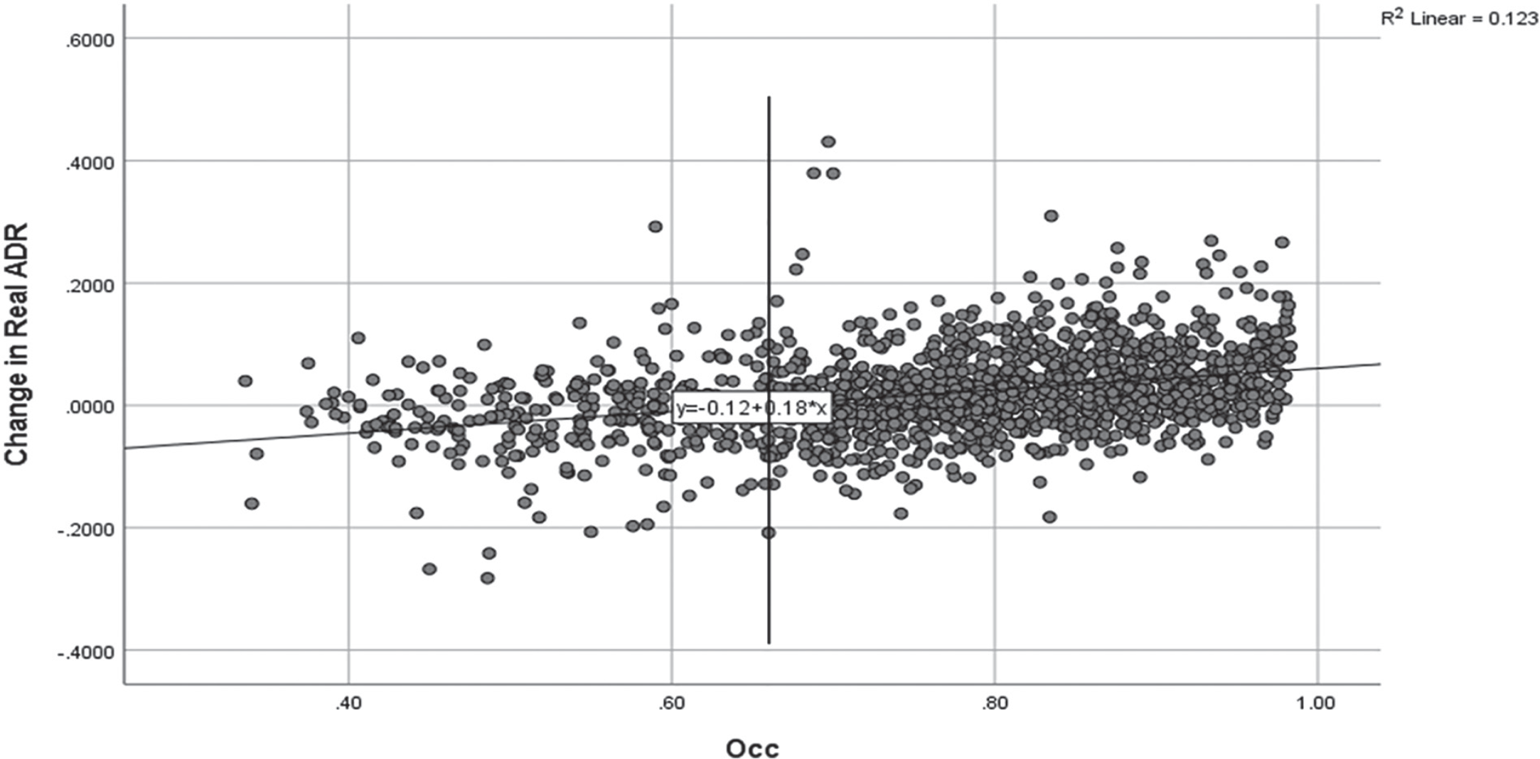
Current Year Occupancy Rate Regressed on Change in Real ADR.

Several interesting observations can be derived from Graph 2. The pattern of observations supports the theory of a linear relationship between occupancy and average rate growth. However, a large proportion of observations are not explained by established natural occupancy rate theory. Specifically, when occupancy levels were greater than 65.7%, the levels of real average rate growth ranged from −21% to +43%, with 34% of the observations being negative. Conversely, when occupancy levels were below 65.7%, average rate growth ranged from −28% to +29%, with 40% of the observations being positive. This high proportion of daily observations not being explained by existing theory suggests that a simple equilibrium threshold is insufficient to fully predict average rate growth and that change in occupancy from the prior year may affect average rate growth above the effect of the absolute occupancy level.

Hypothesis and Development of a Two-Predictor Model

To further explore factors related to relative occupancy levels, bivariate correlations were assessed between daily real ADR growth and current occupancy levels and prior year occupancy levels as well as the relative change in occupancy from the prior year. Table 4 shows the coefficients of correlation between real ADR growth and these predictor variables for the Seattle MSA:

Table 4.

Correlations Between Seattle MSA Occupancy Factors and Daily Real ADR Growth Rates (2014–2018).

Independent Variables	Real average rate growth	Current occupancy	Prior year occupancy
Current occupancy	.35**
Prior year occupancy	.02	.91**
Change in occupancy	.73**	.15**	−.27**

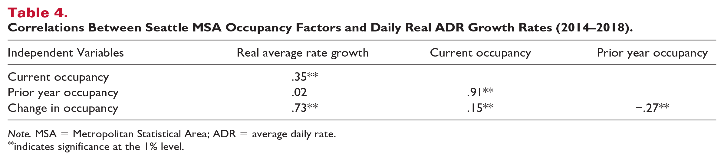
Note. MSA = Metropolitan Statistical Area; ADR = average daily rate.

indicates significance at the 1% level.

Table 4 provides further evidence that current year occupancy levels are more reliable predictors of average rate growth (r = .35, p < .001) than prior year occupancy levels (r = .02, p = .43). In addition, very strong correlations were derived between average rate growth and change in occupancy (r = .73, p < .001), suggesting that the addition of this variable to the model improves predictive power. These correlations provide support for expressing average rate growth as a function of a combination of current occupancy levels and relative change in occupancy levels to further explain the phenomenon of average rates declining even when the market is functioning at high-occupancy levels.

Conceptual Model

The conceptual model being evaluated is represented in Figure 1.

Figure 1.

Conceptual Model of Interaction Between Occupancy and Change in Occupancy in Predicting Change in Average Rates.

This model indicates that occupancy and change in occupancy each predict change in the average rate and that there is an interaction between the variables, with the effect of occupancy depending upon the level of change in occupancy levels from prior years.

Testing of the Conceptual Model

The daily occupancy and average rate observations for the Seattle MSA were analyzed using IBM-SPSS software and Hayes’ PROCESS Model 1. Occupancy observations were deviated by subtracting the natural occupancy rate of 65.7% from each observation so that a threshold-deviated occupancy of 0 represents an observed occupancy rate of 65.7%, and scores above or below 0 represent the degree to which the observed occupancy rate was above or below the natural occupancy rate. This calculation was performed to improve the interpretability of the coefficients and to identify whether the effects of change in occupancy were main effects or simple effects (Spiller et al., 2013). The final regression equation is expressed as $O C C_{t - 1}) + b_{3} (D O C C_{t}) (O C C_{t} - O C C_{t - 1})$ , where DOCC_t represents the current threshold-deviated occupancy rate. The coefficient b₀ represents the real average rate growth when occupancy is at the natural occupancy rate threshold of 65.7% and there is no change from year to year (at which point, the b₁, b₂, and b₃ coefficients would all collapse and the equation would be ΔRADR_t = b₀).

The prediction model shows significantly higher reliability in predicting change in average rates (R² = .61, compared with the single-predictor model R² = .12), suggesting that the level of change in occupancy explains a large proportion of the change in the average rate exceeding the absolute occupancy level.

The results (see Table 5) indicate a significant main effect of occupancy (B = 0.13, p < .001), a significant simple effect of change in occupancy (B = 0.51, p < .001) when occupancy is at the natural occupancy rate, and a significant interaction effect between occupancy and change in occupancy (B = 0.68, p < .001). A one-unit change in occupancy above (below) the natural occupancy rate predicts an increase (decrease) in average rates of 0.13% because of the absolute occupancy level, and a one-unit increase (decrease) in occupancy relative to the previous year predicts a 0.51% increase (decrease) in average rates because of the relative change in occupancy. Furthermore, as absolute occupancy levels increase, the strength of this indirect effect becomes more significant as a result of the positive DOCC × ΔOCC coefficient.

Table 5.

Test for Moderation.

Model 3
Outcome variable	Real change in average rate
Predictor variable	Current year occupancy (threshold-deviated)
Moderator	Change in occupancy
	R ²	MSE	F	p value
Model results	.61	0.00	761.4	.00
Predictors	B	SE	T	p value
Constant	0.00	0.00	1.85	.06
DOCC	0.13	0.01	15.50	.00
ΔOCC	0.51	0.01	39.52	.00
DOCC × ΔOCC	0.68	0.09	7.19	.00

Note: DOCC = threshold-deviated occupancy; ΔOCC = change in occupancy.

As a practical example of the influence of this indirect effect, an annual occupancy rate of 70% results in a prediction of real average rate growth of 0.7% using the single-predictor model presented in Table 3; however, considering the influence of change in occupancy and the interaction effect results in a prediction of a decline in real ADR of 1.65%. Thus, even though the market would still be above the natural occupancy rate, real average rate growth would be negative rather than positive.

Submarket Analysis

The data in Table 6 suggest that the submarkets within the Seattle MSA have significantly different natural occupancy rates, effects of occupancy and occupancy change on average rate growth, and interactions between occupancy and occupancy change. The downtown Seattle submarket indicates a natural occupancy rate of 74.1% as the point that average rate growth would equal inflation in the absence of any increases in either demand or supply. The addition of the change in occupancy and the interaction variables improves the model predictability from R² = .13 to R² = .67 and shows that changes in occupancy have a significantly greater impact on average rate growth than absolute occupancy levels (B = 0.70 vs. B = 0.14). Furthermore, the relationship between change in occupancy and average rate growth becomes stronger at higher levels of occupancy, as indicated by the interaction term (B = 1.61).

Table 6.

Test for (1) Natural Occupancy Rates and (2) Moderation Across Submarkets.

Model 4a(1)—Downtown Seattle				Model 4a(2)—Downtown Seattle
	R ²	F	p value		R ²	MSE	F	p value
Model results	.13	217.63	.000	Model results	.67	0.01	386.21	.000
Predictors	B	SE	p value	Predictors	B	SE	T	p value
Constant	−0.19	0.01	.000	Constant	0.01	0.00	2.24	.03
Occupancy	0.25	0.02	.000	DOCC	0.14	0.01	11.40	.00
Equil. level	74.1%			ΔOCC	0.70	0.02	36.53	.00
				DOCC × ΔOCC	1.61	0.12	13.00	.00
Model 4b(1)—Eastside				Model 4b(2)—Eastside
	R ²	F	p value		R ²	MSE	F	p value
Model results	.08	119.97	.000	Model results	.09	0.04	47.20	.000
Predictors	B	SE	p value	Predictors	B	SE	T	p value
Constant	−0.08	0.01	.000	Constant	0.00	0.02	0.69	.49
Occupancy	0.11	0.01	.000	DOCC	0.10	0.01	9.07	.00
Equil. level	76.6%			ΔOCC	0.06	0.03	2.43	.02
				DOCC × ΔOCC	−0.38	0.16	−2.44	.02
Model 4c(1)—SeaTac Airport				Model 4c(2)—SeaTac Airport
	R ²	F	p value		R ²	MSE	F	p value
Model results	.09	137.37	.000	Model results	.24	0.45	157.4	.00
Predictors	B	SE	p value	Predictors	B	SE	T	p value
Constant	−0.09	0.01	.000	Constant	0.00	0.00	0.47	.64
Occupancy	0.14	0.01	.000	DOCC	0.11	0.01	10.37	.00
Equil. level	61.9%			ΔOCC	0.29	0.03	8.82	.00
				DOCC × ΔOCC	0.78	0.19	4.22	.00

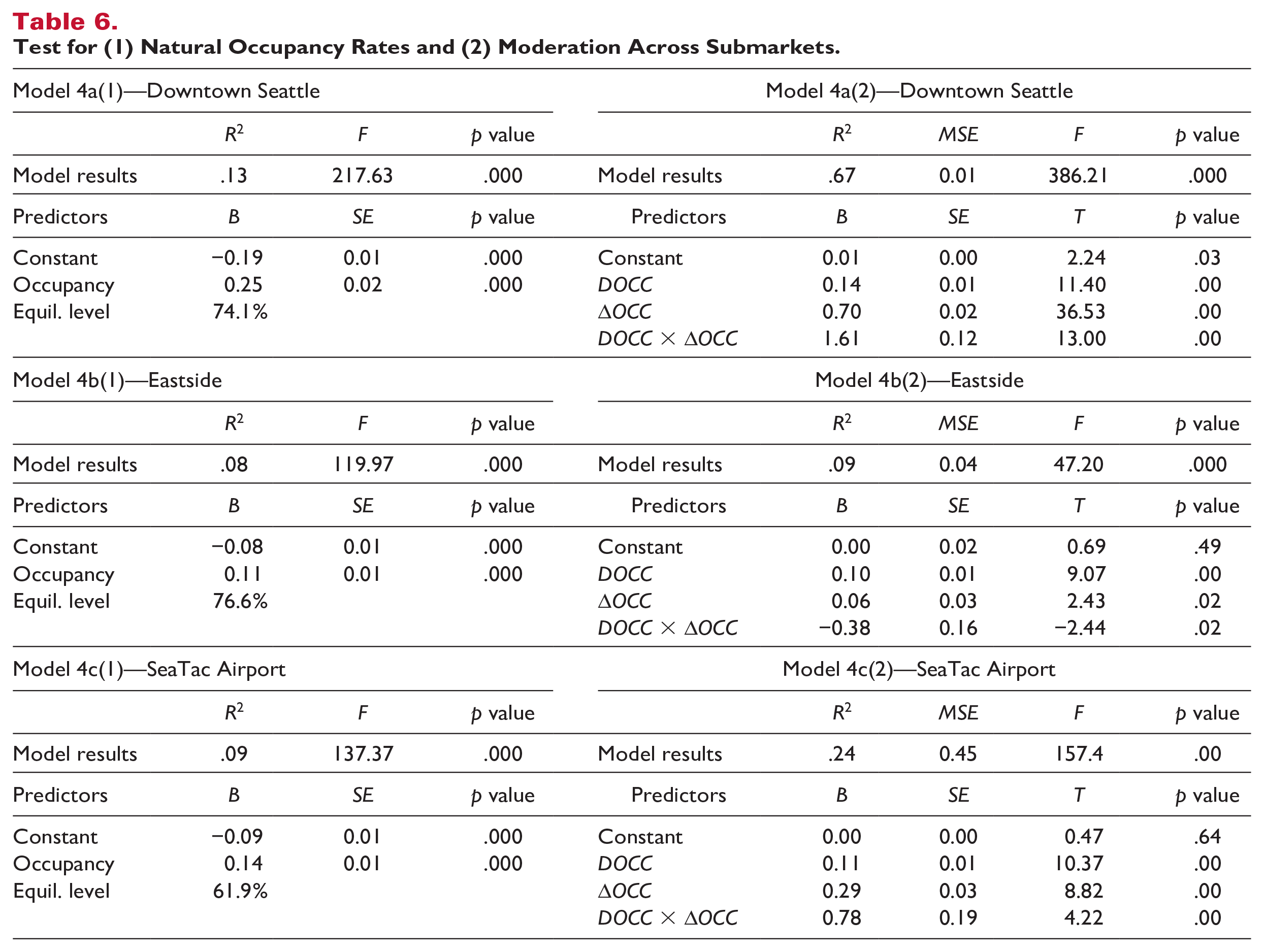
For the Eastside of Seattle, the natural occupancy rate was determined to be 76.1%, but in this submarket, the addition of the predictors did not significantly improve the model (ΔR² = .01). Occupancy and change in occupancy within the submarket have lesser impacts on average rate growth than found in the MSA or the downtown Seattle submarket, and the significant and negative coefficient for the interaction term indicates that the relationship between change in occupancy and average rate growth becomes weaker at higher levels of occupancy and stronger at lower levels of occupancy. These results suggest that the Eastside might operate less independently with more interlinkages between other submarkets. Thus, the Eastside would be influenced by external factors such as the overall MSA demand/supply balance or by trends in an adjacent central business district.

The SeaTac Airport submarket was determined to have the lowest natural occupancy rate of the submarkets studied, at 65.9%, and the addition of the change in occupancy and the interaction term improved the model reliability from R² = .09 to R² = .24. As with the Seattle downtown and MSA markets, changes in occupancy are more consequential to average rate growth in the airport submarket than the absolute occupancy rate (B = 0.29 vs. B = 0.11), and the positive interaction term indicates that the relationship between change in occupancy and average rate growth becomes stronger at higher levels of occupancy.

Conclusion

Conventional wisdom on natural occupancy rates and market equilibrium suggests that average rate growth is positive if a market is operating above its natural occupancy rate. This study provides evidence that real average rate growth is also influenced to a significant degree by the indirect effect of changes in occupancy from year to year. A market that is declining in occupancy but still above its natural occupancy rate may well experience declines in real average rates as a result of the moderating influence of change in occupancy rates. Assuming that a market will experience real average rate growth simply because it is operating above its natural occupancy rate without considering the relative change in occupancy levels from prior years may lead to erroneous planning and pricing decisions by management and ownership.

Implications

This research has several implications for academia and industry. Understanding the dynamics of average rate growth is fundamental to assessing the relative health of lodging markets, forecasting future revenues for existing and potential new hotels, and managing hotel room inventory to optimize revenues and profitability. To that end, incorporating the influence of relative occupancy levels on average rate growth into future revenue assumptions can help practitioners avoid overestimating or underestimating future revenue potential and thereby making incorrect decisions.

Specifically, owners or managers setting expectations for hotels or potential hotels in markets that have benefited from above-inflationary rate growth for a prolonged period may become overly accustomed to the benefits of average rate growth and may be unprepared for the impact on average rate growth that occurs when occupancies decline, even if they remain at relatively high levels. Simply assuming that rates will increase because the market is operating above its natural occupancy rate may lead to overestimating future revenues and inaccurate assessment of management performance.

Similarly, developers and regional planners charged with maintaining balanced growth in a market should consider the effect of even modest occupancy declines on market rate growth, even if the market remains above the theoretical natural occupancy rate. Taking a simplistic approach to evaluating development opportunities based on performance relative to the natural occupancy rate obscures potential impacts of changing occupancy levels on average rate growth above the absolute occupancy level that could lead to catastrophic planning decisions.

Limitations and Future Research

The primary limitation of this study is the focus on a single lodging market and a limited period of time. As with any case study research, conclusions drawn from one market may not generalize well to other markets, and replication is necessary to confirm the reliability of the conclusions. Furthermore, although the predictive ability of the multiple-predictor regression equations is significantly higher than that of single-predictor models, a large proportion of the variability of ADR growth remains to be explored.

Consistent with the findings of deRoos (1999), this study shows that submarkets within the Seattle MSA have different natural occupancy levels but does not explore factors that contribute to these differences. This study also does not explore differences between hotel quality levels or the potential for natural occupancy levels to shift over time or during periods of recession or alternative regimes (Gallagher & Corgel, 2018). Similarly, segmenting hotels by demand segments (commercial, leisure, and group) or quality level may show dramatically different impacts as well as different vulnerability levels to occupancy shifts.

The confirmation of a moderation effect shows that the change in occupancy is a significant factor in average rate growth, but this interaction merits further investigation. Whether occupancy change is driven by changes in supply or by changes in demand may cause different market reactions and influences on rate growth, and studying the magnitude of the occupancy change may provide further insights. Specifically, it would be reasonable to expect that a 10% increase or decrease in occupancy may be proportionately more impactful than a 1% change. In addition, the impacts of occupancy change are likely to be asymmetric based on the level of occupancy or the direction of occupancy change. If a market is operating at a high- or low-occupancy level, increases in occupancy may be more or less impactful than declines, and rates may be more elastic during periods of decline as hotels may become more aggressive in their pricing strategies.

Finally, the different levels of reliability and significance of the predictor variables between submarkets merit further investigation. Particularly, in the case of the Eastside where hotels may be interacting with other submarkets outside of the submarket or may have other factors (changes in demand generators, transportation modes, or overall desirability) confounding the results, researchers need to develop a deeper understanding of intraregional rate growth dynamics to assess how supply growth in one submarket may influence revenues in interdependent submarkets.

Footnotes

Declaration of Conflicting Interests

The author(s) declared no potential conflicts of interest with respect to the research, authorship, and/or publication of this article.

Funding

The author(s) received no financial support for the research, authorship, or publication of this article.

ORCID iD

Gregory Denton

Author Biographies

Gregory Denton is Managing Director of the Arden Group, and a PhD student in the Hospitality Business Management program at Washington State University. He received his BS and MS degrees from Cornell University.

Jennifer Sandstrom is Clinical Assistant Professor in the Hospitality Business Management program at Washington State University Vancouver. Dr. Sandstrom’s research focuses on hotel General Manager leadership, hotel culture, hotel performance, and hospitality education.

References

Arenoe

van Der Rest

J.-P.

Kattuman

(2015). Game theoretic pricing models in revenue management: An equilibrium choice-based conjoint analysis approach. Tourism Management, 51, 86–102.

Buckhiester

(2011a). Revenue management as a multi-disciplinary business process. Journal of Hospitality Financial Management, 19(1), 91–103.

Buckhiester

(2011b). Revenue management as a multi-disciplinary business process: Part two. Journal of Hospitality Financial Management, 19(2), 97–113.

Chen

C. M.

Chang

K. L.

(2012). The effect of price instability on hotel profitability. Tourism Economics, 18, 1351–1360.

Chen

C. M.

Chiu

H. H.

(2014). Market disequilibrium effect on hotel prices. Tourism Economics, 20(4), 901–909.

Corgel

(2005). Hotel real estate markets. The Journal of Portfolio Management, 31, 91–99.

Corgel

deRoos

(1993). The ADR rule-of-thumb as predictor of lodging property values. International Journal of Hospitality Management, 12(4), 353–365.

deRoos

(1999). Natural occupancy rates and development gaps. Cornell Hotel and Restaurant Administration Quarterly, 40(2), 14–22.

Erdem

Jiang

(2016). An overview of hotel revenue management research and emerging key patterns in the third millennium. Journal of Hospitality and Tourism Technology, 7(3), 300–312.

10.

Gallagher

Corgel

(2018). Natural occupancy shifts in hotel markets. Cornell Hospitality Quarterly, 59(4), 352–363.

11.

Kalcevic

(2018). The hotel lodging cycle. https://www.todayshotelier.com/2018/01/01/the-hotel-lodging-cycle/

12.

Kimes

S. E.

(1989). The basics of yield management. Cornell Hotel and Restaurant Administration Quarterly, 30(3), 14–19.

13.

Kimes

S. E.

(2015). The evolution of hotel revenue management. Journal of Revenue and Pricing Management, 15(3–4), 247–251.

14.

Lee

S. K.

Jang

(2011). Room rates of U.S. airport hotels: Examining the dual effects of proximities. Journal of Travel Research, 50(2), 186–197.

15.

Lee

S. K.

Jang

(2012a). Premium or discount in hotel room rates? The dual effects of a central downtown location. Cornell Hospitality Quarterly, 53(2), 165–173.

16.

Lee

S. K.

Jang

(2012b). Re-examining the overcapacity of the US lodging industry. International Journal of Hospitality Management, 31, 1050–1058.

17.

W. Y.

(1961). The desirability of price instability under perfect competition. Econometrica, 29(1), 58–64.

18.

Rosen

(1974). Hedonic prices and implicit markets: Product differentiation in pure competition. The Journal of Political Economy, 82(1), 34–55.

19.

Shoval

(2006). The geography of hotels in cities: An empirical validation of a forgotten model. Tourism Geographies, 8(1), 56–75.

20.

Spiller

Fitzsimmons

Lynch

McClelland

(2013). Spotlights, floodlights, and the magic number zero: Simple effects tests in moderated regression. Journal of Marketing Research, 50, 277–288.

21.

Tisdell

(1963). Uncertainty, instability, profit. Econometrica, 31, 243–247.

22.

Wheaton

Rossoff

(1998). The cyclic behavior of the U.S. lodging industry. Real Estate Economics, 26, 67–82.