Method to evaluate the effect of inclination angle of steel open-type check dam on debris flow impact load

Abstract

Although the latest statistics indicate a decrease in the number of victims of natural disasters in Japan, the number of sediment disasters has increased. A countermeasure against natural disasters is provided by the installation of a steel open-type check dam (hereafter, open Sabo dam). The open Sabo dam is expected to capture boulders (more than 1.0 m in diameter) contained in debris flow of which boulders concentrate in front part. When a debris flow impacts an open Sabo dam, the large impact load on the steel pipes are caused by the impact of boulders under debris flow. Therefore, it is important to evaluate the impact of both boulders and the following soil and small gravels including fluid force of the open Sabo dam from the design point of view. Although an open Sabo dam has various shapes especially, the every open Sabo dams is evaluated by the same design method in Japan. It is necessary to propose the load evaluation method in the experiment scale in contrast with different shape of open Sabo dam. This article presents an experimental approach to determine the effect of the front inclination angle of steel open Sabo dams on the impact load. The debris flow impacts 1/40 scale models of steel open Sabo dams which are set in a flow channel flume, and the debris flow load is measured by using three load cells placed horizontally at the back of the Sabo dam model. Different front inclination angles are set for each Sabo dam models. The time history of the impact load is examined by comparing the loads corresponding to four kinds of dams, which are different from the front inclination angles, and decrease of impact load considering the buffering effect of driftwoods in debris flow.

Keywords

Debris flow load steel open Sabo dam front inclination angle woody debris flow boulder

Introduction

Although the latest statistics indicate a decrease in the number of victims of natural disasters in Japan, the number of sediment disasters has increased. Especially, the debris flow including driftwood has a large impact force. For example, a debris flow including a large amount of wood recently caused significant damage in the Kyusyu area and invaded the area of residences in July 2017 (National Institution for Land and Infrastructure Management, Ministry of Land, Infrastructure, Transport and Tourism, 2017). In addition, the woody debris flow was generated by a typhoon in Kagoshima city in July 2016. Furthermore, a large amount of damage occurred in the Kirishima district. Such disaster situations highlight the necessity to study debris flows and woody debris flows (National Institution for Land and Infrastructure Management, Ministry of Land, Infrastructure, Transport and Tourism, 2016). One of such countermeasures against debris flow is the construction of a steel pipe check dam (hereafter, open Sabo dam) as shown in Figure 1. The associated mechanism allows the flow of water, soil, and small gravel for maintaining the flow of the river. But, when the debris flow occurs, the open Sabo dams are expected to capture boulders which are concentrated in the front part of debris flow, and the following sand and gravels can be caught by blocking the penetration part (slit part) of the open-type Sabo dam.

Figure 1.

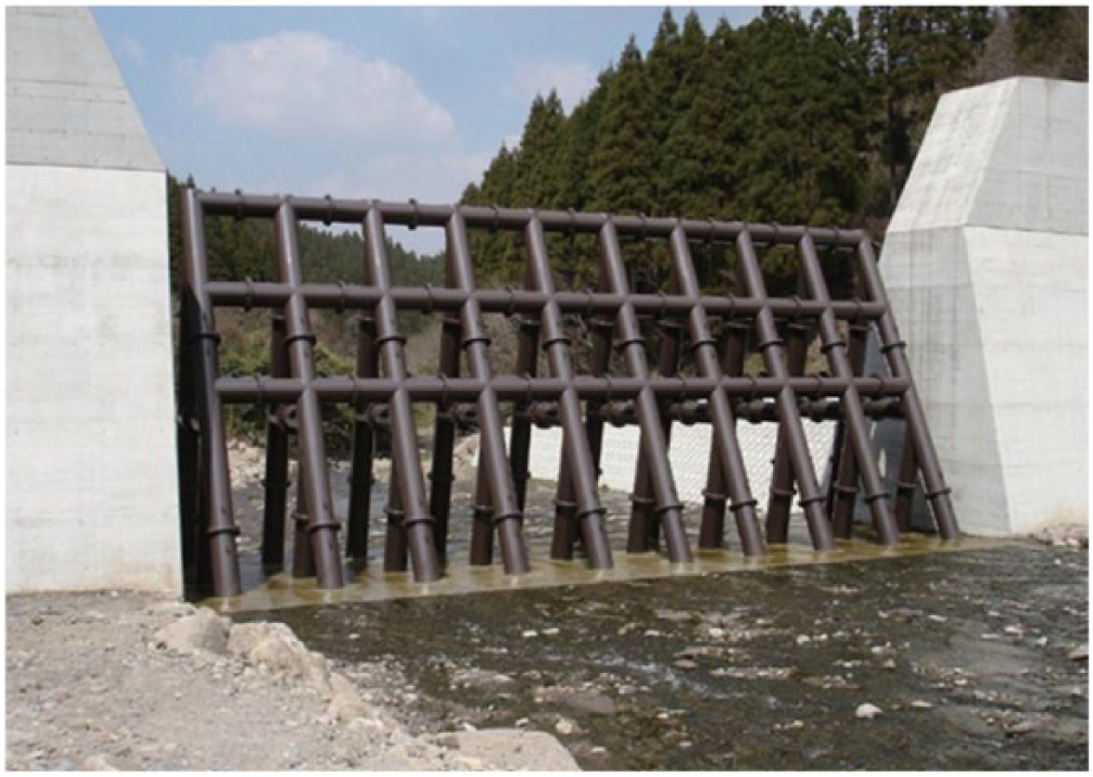
Steel open-type check dam.

Figure 2 shows a damaged steel part of open Sabo dam in the Nagiso region, Nagano prefecture, Japan. The dam prevented the debris flow to cause damage in the region during a downpour in July 2014 (Hiramatsu et al. 2014).

Figure 2.

First Nashizawa Sabo dam struck by a natural disaster.

Although the Sabo dam received big impact loads in the same mountainous area, the open Sabo dam as shown in Figure 3 caught the boulder in debris flow. The Sabo dam has not been greatly destroyed. This means that the impact load has been reduced by some mechanisms. Compared to the open Sabo dams shown in the Figures 2 and 3, the destruction situation are greatly different. The different reason is thought to be the speed, height of the debris flow, and the angle of the mountain, but the main reason is the difference between the front inclination angles of the open Sabo dams.

Figure 3.

Second Nashizawa Sabo dam in Nagiso.

In the Japanese design, the debris flow can have two interpretations method. Ikeya (1978) categorized debris flow load in terms of the fluid theories and solid theories. Each classification was used to calculate the impact force of a debris flow for a concrete Sabo dam (hereafter, closed Sabo dam). The impact force of the boulder is calculated using the solid theory, considering the energy of the partial destruction under collision (Mizuyama, 1979). In addition, Daido et al. (1992) evaluated the pressure of debris flow acting on a flat face of closed Sabo dam. The debris flow was regarded as either an incompressible fluid or a compressible fluid (Daido et al., 1992) and provided a method to determine the impact force. An experimental evaluation equation is introduced based on these results, and there are some research that compare the debris flow load of the experiment with the present design method (Yamamoto et al., 1998). In a basic research of the debris flow considering design load, Mizuyama et al. (1995) and Iwamoto and Hirano (1982) proposed two classifications for the debris flow load evaluation considering a steel pipe type Sabo dam. The two classifications divide fluid force evaluation and boulder impact load evaluation. The two classifications divide fluid force and boulder impact load. Moreover, Wada et al. (2015) indicated that the segregation is caused owing to a large particle flow mixing with that of minute particles, wherein the large particles accumulate in the initial zone of the debris flow. In addition, Shima et al. (2014) carried out flume experiments with sediment mixtures and investigated the gravel diameters and steel pipe intervals where the boulder was captured in a steel open Sabo dam. Moreover, Shibuya et al. (2012) examined an experimental approach on the load exerted by a debris flow with woody debris flow on open Sabo dam of steel frames. The hydraulic model experiments were carried out with various parameters, driftwood containment ratios of debris, and slit intervals of the structure. When the debris flow contains woody debris, the driftwoods accumulate in the front of the debris flow, and the slit of the structure is blocked by the captured woods. Furthermore, the impact load caused by debris flow with woody debris flow is smaller than that of debris flow. It is thought that driftwood becomes a cushioning material and reduced the impact load. Miyoshi and Suzuki (1990) proposed a method to evaluate the deformation of the flow and the impact load on the dam. In this model, the initial conditions (depth of debris flow and sediment density) are expressed in functional relationships experimentally, and the load is estimated quantitatively. The experimental results of debris flow, load on the dam, and their variation with time calculated by this model have proven to agree well with those observed or measured in experiments. Beppu et al.(2011) carried out a numerical simulation of a debris flow model by using the modified moving particle semi-implicit (MPS) method with solid and liquid particles. Herein, the contact between the solid particles and the frictional force between the solid particles and the surface are taken into account. The proposed method could reproduce the surge formation in the debris flow model and determine the load time history. Therefore, the fluid force using MPS and the gravel collision load using distinct element method (DEM) are examined in the analysis. But, the analysis and gravel in two-dimension (2D) are considerably different from the actual phenomena. In addition, Mizuyama et al. (1985) used various inclinations between the fluid force and the structure for the case of a boulder colliding with the steel open Sabo dam and measured the flow velocity and pulse height at the instant. Moreover, they conducted experiments that reproduced the surge shape and analyzed the soil pressure in damp or wet conditions. The article presented to differ the impact load evaluation due to the difference of surge-type debris flow and no-surge-type debris flow. However, extant studies did not consider experimentally the influence of the front shape of an open Sabo dam, especially the corner, and the corresponding shock impact load.

This paper presents an experimental approach to determine the effect of the front inclination angle of open Sabo dams on the impact load. A model of debris flow composed of boulder and driftwood is developed. Each different inclination angles of the front plane are set for each dam model. The time history of impact load is analyzed by comparing the loads corresponding to different inclination angles.

Outline of experiment

Experiment of flume

The channel flume shown in Figure 4 uses a variable slope straight line. The length, width, and depth of the channel flume are 4.5 m, 30 cm, and 50 cm, respectively, and the channel slope, which can be set using the river bed slope, was same as the Nashizawa river slope (θ = 11.3°). The debris flow model use gravels and woods as shown in Figure 8. The way of flowing is to pour water from the rear side of the gravel. The bed roughness is arranged at the bottom of the flume. The surge shape of the debris flow was made by using the bed roughness referring to the research of Adachi (1964). The interval of the bed roughness that spreads the channel flume had an opening of 30 mm, height 5 mm, as shown in Figure 4. The length of the bed roughness extended 2.0 m from the dam. The dam model and the load measurement points are shown in Figures 5 and 6. The debris flow load was measured using two load cells and one component force meter placed symmetrically downstream of the Sabo dam model. Moreover, the dam model was placed in the top part of the flume to avoid friction with the bottom plate, as shown in Figures 5 and 6. In other words, the horizontal force exerted on the dam model by the debris flow was measured using three load cells. The three load cells are hung from the upper part of experimental device.

Figure 4.

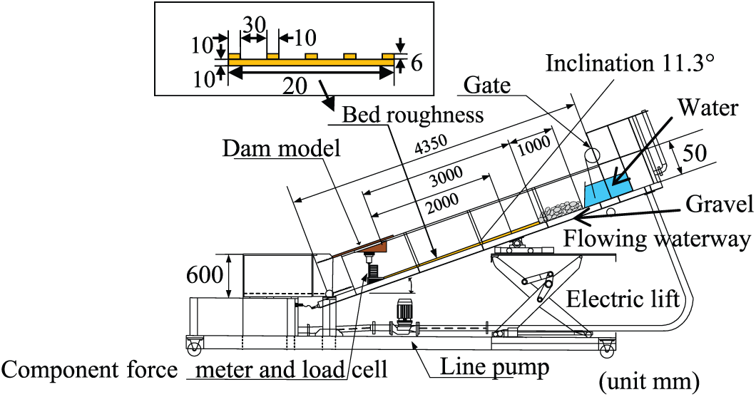
Experimental flume.

Figure 5.

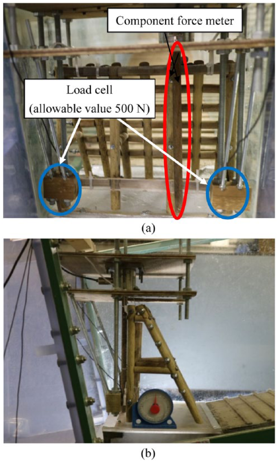
Experimental device: (a) rear side and (b) left side.

Figure 6.

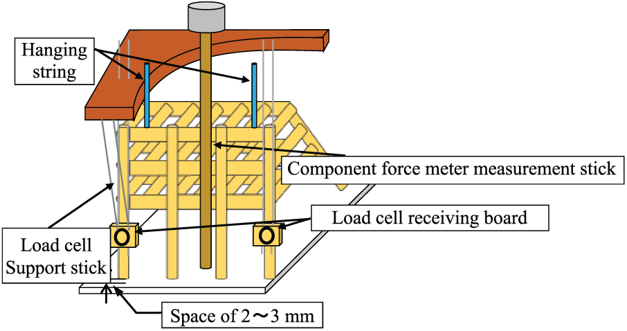
Sabo dam model.

Dam model

The four dam models (A, B, C, D) are shown in Figure 7. The main parameter considered was the front inclination angle θ_LS, which was varied between 0° and 30°. The dam model was fixed and constructed wooden round bar of 16 mm. The front shape involved seven vertical columns at equal intervals of 30 mm. Therefore, the four models are different from front inclination angle. The trapping performance is determined by the horizontal base material. Thus, the configuration of the horizontal material was considered along with the influence of the horizontal bracing, and trapping performance is separately discussed. Here, this article focuses on the impact load of open Sabo dam.

Figure 7.

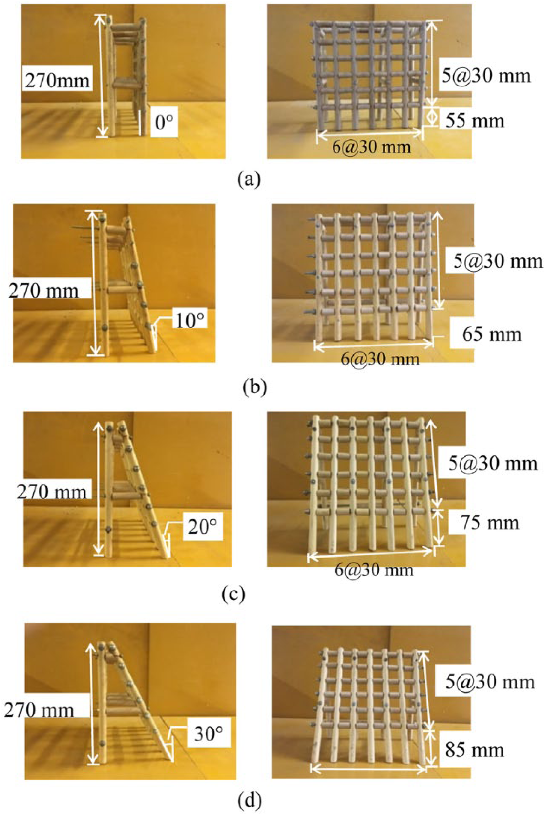
Dam model: (a) Model A (θ_LS = 0°), (b) Model B (θ_LS = 10°), (c) Model C (θ_LS = 20°), and (d) Model D (θ_LS = 30°).

Debris flow model

The gravel models and wood models are shown in Figure 8. The parameters of each experiment are shown in Table 1. The model shown in Figure 9 had average grain diameters of 10, 20, and 30 mm, and the grain size sedimentation curve is also shown. The specific gravity of the gravel material was specific gravity 2.6 (unit of measurement), and gross weight of the entire gravel was 35 kg. The diameter, length, and specific gravity of the driftwood was 6, 120 mm, and 0.98 (unit of measurement), respectively. The gross wood of the driftwood was 500 sticks, and it encompassed 10% of the volume of the debris flow. Two kinds of debris flow states were considered in the experiment: debris flow and woody debris flow.

Figure 8.

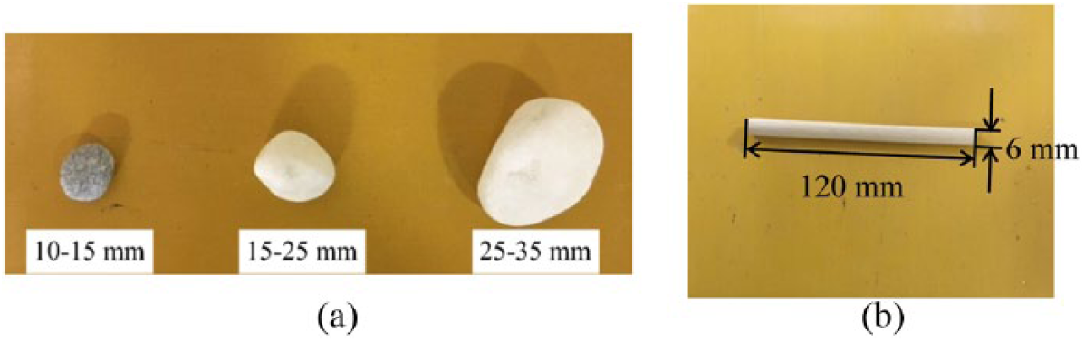
Test pieces: (a) gravel model and (b) wood model.

Table 1.

Unit of mesurements.

Name	Specific gravity	Grain diameter	Mass
Gravel model (small)	2.6	15 mm	16 kg
Gravel model (middle)		16–25 mm	12 kg
Gravel model (large)		26 mm	7 kg
Driftwood model	0.98	ϕ = 6 mm, l = 120 mm	500

Figure 9.

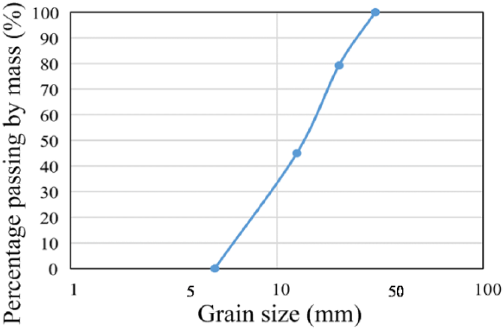
Grain size distribution.

Figure 4 is indicated that the gravels and driftwoods were set up from the dam to upstream of 3.0 m. The discharge was 0.06 m³/s. The debris flow impact is 1/40 scale models of the steel open Sabo dam. This experiment scale follows fluid similarity rule.

Experiment cases

The experiment was divided into eight cases as shown in Table 2, and the experiment was performed five times for each cases to ensure reproducibility. Thus, the experimental cases represented different combinations of the Sabo dam model and the debris flow conditions.

Table 2.

Experiment case.

Front angle	Case	Dam	Debris flow	Discharge
θ_LS = 0°	G-0°	Model A	Gravel	0.06 m³/s
θ_LS = 10°	G-10°	Model B
θ_LS = 20°	G-20°	Model C
θ_LS = 30°	G-30°	Model D
θ_LS = 0°	G_W-0°	Model A	Driftwood and gravel
θ_LS = 10°	G_W-10°	Model B
θ_LS = 20°	G_W-20°	Model C
θ_LS = 30°	G_W-30°	Model D

Number of experiment is each five.

Experimental result

Shape of sedimentation

Figure 10 shows the comparison of inclination angles of the dam considering the shape of sedimentation against debris flow in the experiment. In terms of the inclination angle, for θ_LS = 0° and 30°, the sedimentation height of the dam impacted upon debris flow is 192 and 215 mm, respectively. A larger front inclination angle of the dam corresponded to a higher sedimentation. Also, the height of sedimentation was judged based on the photo. The height shows the part where the dam has come in contact. Here, the height of sedimentation contacted Sabo dam is static sedimentation load of debris flow in Japanese design.

Figure 10.

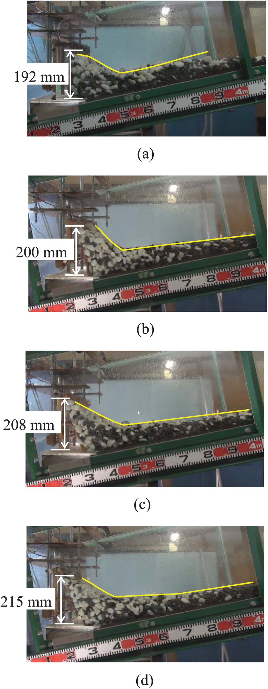
Final sedimentation shape (debris flow): (a) inclination angle θ_LS = 0°, (b) inclination angle θ_LS = 10°, (c) inclination angle θ_LS = 20°, and (d) inclination angle θ_LS = 30°.

Therefore, the reason of decreases in load is the impact load because of the delay to final shape of sedimentation. However, a larger front inclination is necessary to ensure that the gravels do not overflow the Sabo dam. For all experiments, the sedimentation shape was indicated by a yellow line in Figure 10.

The comparison of the front inclination angles of the Sabo dam models is shown in Figure 11, considering the final sedimentation shape in woody debris flow.

Figure 11.

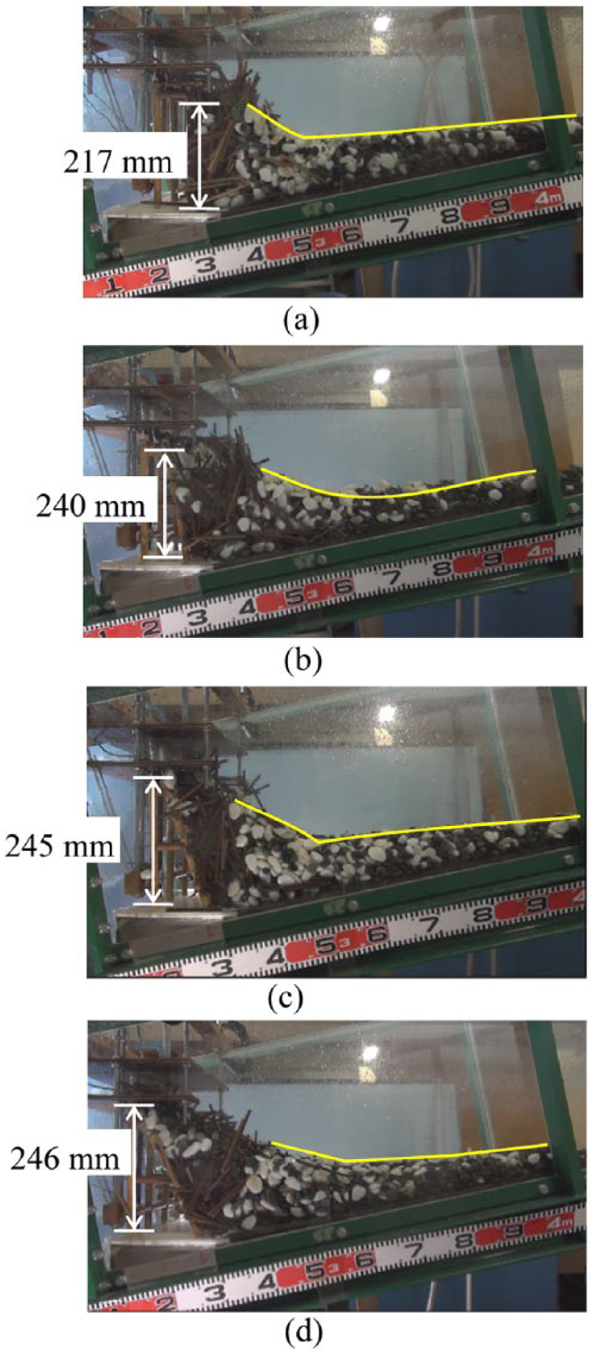
Final sedimentation shape (woody debris flow): (a) inclination angle θ_LS = 0°, (b) inclination angle θ_LS = 10°; (c) inclination angle θ_LS = 20°, and (d) inclination angle θ_LS = 30°.

The driftwood reaches first and is caught in the front part of the Sabo dam. In addition, in all cases, the big gravels are caught on the upstream side. However, compared to case of a small inclination (θ_LS = 0°) and the case of a large inclination (θ_LS = 30°), the sedimentation height of driftwood is seen to increase. The debris flow experimental conditions are repeatable for all experimental cases, and this difference of debris flow load appears in the interaction of driftwoods and gravels. Therefore, the impact load of debris flow are a little due to shape of Sabo dam and the flowing material (e.g. gravel or wood), respectively. The difference in the time that the driftwood rises and the time of arrival of the gravels is small, and the pressing action of the gravel that follows driftwood at the height is effective.

Process of trap sedimentation

Figure 12 shows the trapping sedimentation process of model A (θ_LS = 0°) under debris flow conditions. Figure 12(a) shows the time when the front part of debris flow reaches the Sabo dam. The debris flow that approaches the dam forms a surge due to bed roughness. (Figure 12(b)). The following gravels become concentrated and reach the Sabo dam. Especially, the white gravel cased segregation concentrates in the front part of the debris flow and collides with the dam. Figure 12(c) shows the instant of maximum load. The height of the gravels that stop in front of the dam is the maximum. Figure 12(d) shows the instant that the following gravel is caught by the Sabo dam, and water keeps flowing in the space of the gravel. Figure 12(e) shows the halting of debris flow.

Figure 12.

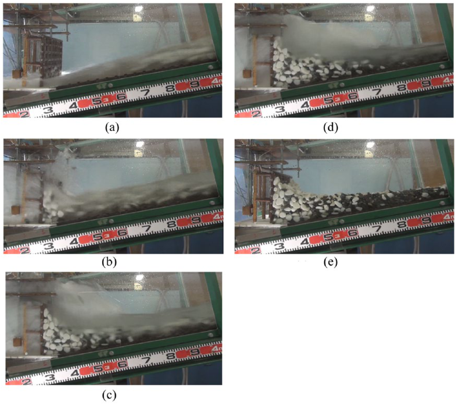
Trapping sedimentation process (G-0°): (a) t = t₀ s, (b) t = t₀ + 0.3 s, (c) t = t₀ + 1.0 s, (d) t = t₀ + 2.5 s, and (e) t = t₀ + 5.5 s.

Figure 13 shows the trap sedimentation process of model D (θ_LS = 30°) under debris flow conditions. Figure 13(a) shows the same parameters as Figure 12(a). Figure 13(b) shows the moment that the gravel that stops in the front begins to be caught from the lower side of the front side of the dam. Figure 13(c) shows the instant corresponding to the maximum load. Figure 13(d) shows the instant that the gravel is caught by the dam and stops in a manner similar to that by the final shape. In addition, water exits the space and flows. Figure 13(e) shows the lost water and the instant after the gravel has been stopped.

Figure 13.

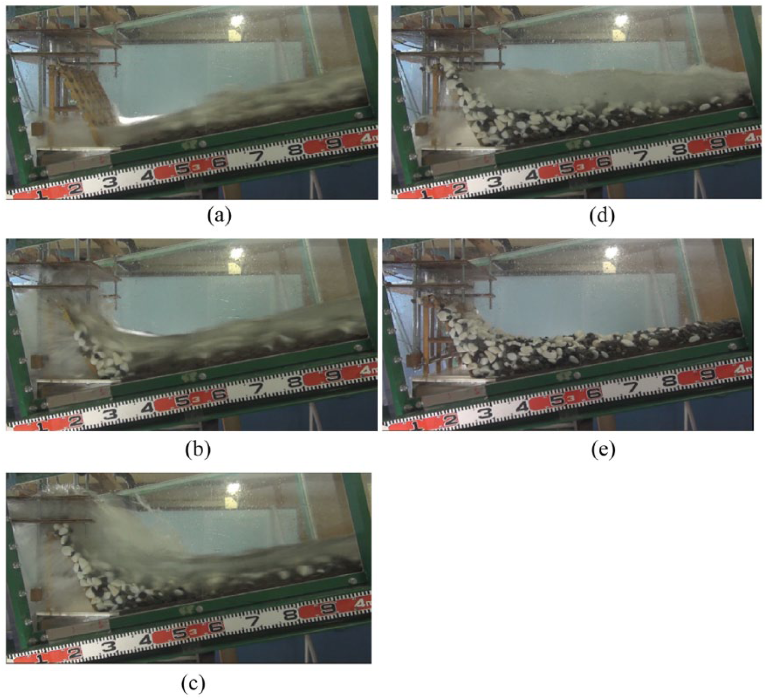
Trapping sedimentation process (G-30°): (a) t = t₀ s, (b) t = t₀ + 0.3 s, (c) t = t₀ + 1.1 s, (d) t = t₀ + 2.5 s and (e) t = t₀ + 5.5 s.

Figure 14 shows the trap sedimentation process of model A (θ_LS = 0°) under woody debris flow conditions. Figure 14(a) shows the debris reaching the dam in the front part of the woody debris flow. The driftwood concentrates on the approaching debris flow and gives rise to a surge. The driftwood rises high in front of the dam as shown in Figure 14(b). Moreover, the gravel, from which the set has been transported, collides with the lower side of the dam. The driftwood then extends to the upper part. Figure 14(c) shows the maximum load. On the downstream side, the following gravel crushes the driftwood that extends up. The driftwoods and gravels are caught by the dam in Figure 14(d). Figure 14(e) shows the final sedimentation shape.

Figure 14.

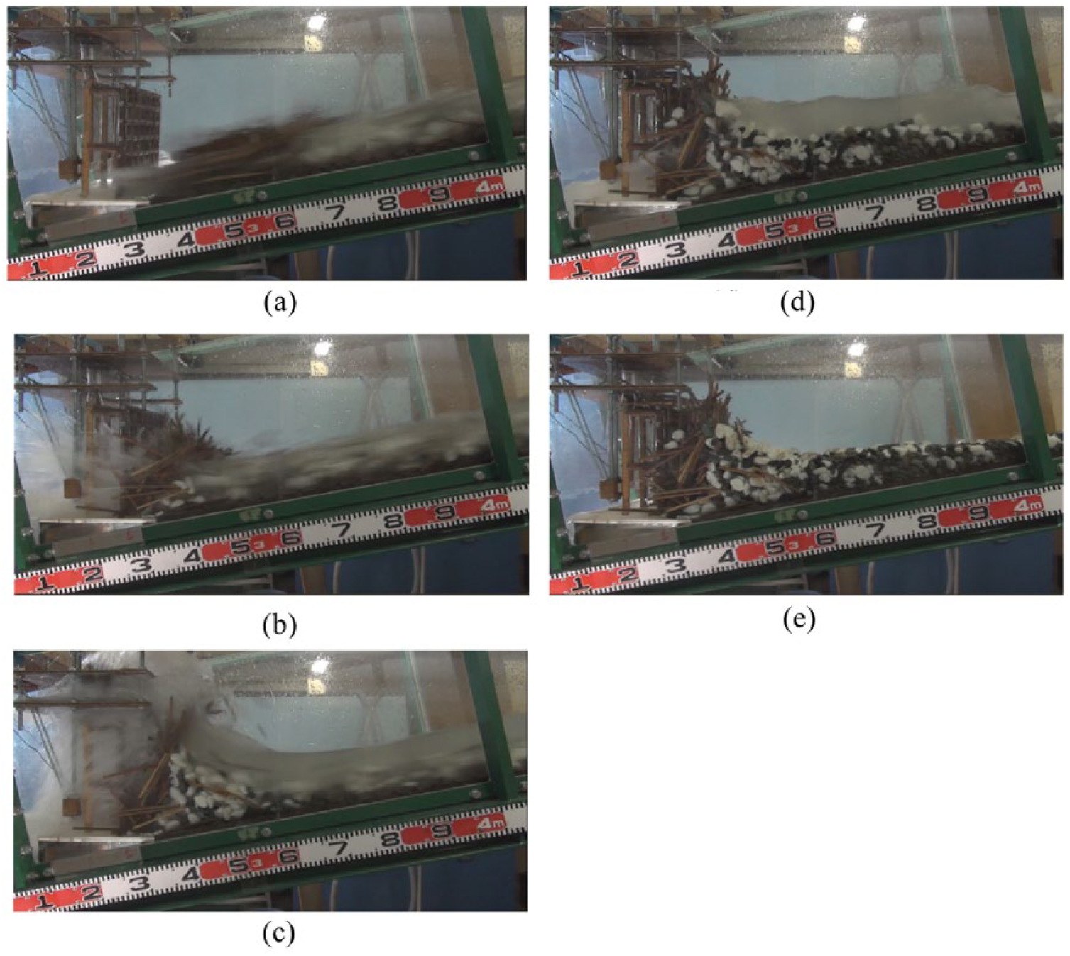
Trapping sedimentation process (Gw-0°): (a) t = t₀ s, (b) t = t₀ + 0.3 s, (c) t = t₀ + 1.1 s, (d) t = t₀ + 2.5 s, and (e) t = t₀ + 5.5 s.

Figure 15 shows the trap sedimentation process of model D (θ_LS = 30°) under woody debris flow conditions. The preceding driftwood stopped, and the following driftwood climbs the accumulation vertically. Moreover, the gravel from which the set is transported collides downward, and the driftwood of the preceding flow stands upright. Therefore, a large space is occupied by the dam and driftwoods stack up. Figure 15(c) shows the maximum load. The driftwood sticks with the following gravels along the dam. Moreover, gravel moves in the driftwood while running aground. Figure 15(d) and (c) represent the same parameters as Figures 12 and 14 and denote a process similar to the ones for all experiment results.

Figure 15.

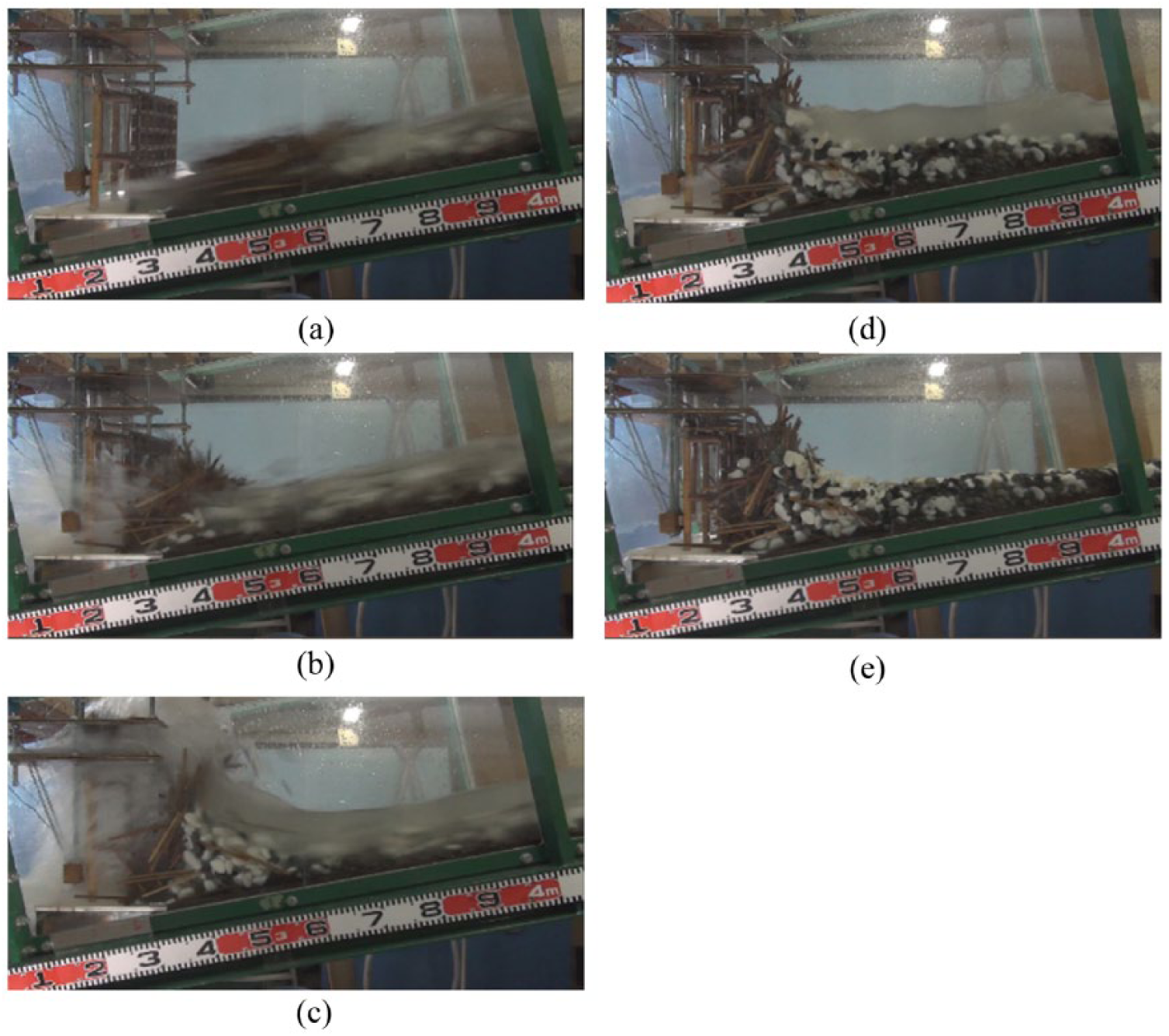
Trapping sedimentation process (Gw-30°): (a) t = t₀ s, (b) t = t₀ + 0.3 s, (c) t = t₀ + 1.3 s, (d) t = t₀ + 2.5 s, and (e) t = t₀ + 5.5 s.

Table 3 indicates the time between the instant of debris flow collision to that corresponding to maximum impact load for all experimental conditions. In case of debris flow, when the inclination angle increases, the time between the collisions to maximum load changes from 0.40 s to 0.82 s. This tendency reduces from 0.27 s to 0.39 s in case of woody debris flow conditions. However, the arrival time is reduced in the case of debris flow.

Table 3.

Time until generating maximum load.

Large division	Case	Experiment(s)					Average(s)
Large division	Case	1	2	3	4	5	Average(s)
Debris flow	G-0°	0.50	0.38	0.34	0.40	0.36	0.40
	G-10°	0.38	0.46	0.32	0.44	0.52	0.42
	G-20°	1.02	0.62	0.78	0.46	0.76	0.73
	G-30°	0.82	0.48	0.74	1.28	0.80	0.82
Woody debris flow	Gw-0°	0.20	0.18	0.20	0.42	0.36	0.27
	Gw-10°	0.34	0.28	0.30	0.30	0.26	0.30
	Gw-20°	0.16	0.38	0.40	0.30	0.36	0.32
	Gw-30°	0.48	0.40	0.48	0.38	0.20	0.39

Time history of impact load

Figure 16 indicate relationship between load and time. Figure 17 indicates the maximum load and sedimentation load (Watanabe et al., 1980) for all experimental cases when considering a reduction in the inclination angle of the dam. The maximum value of the load is the maximum impact load or a dynamic load. The sedimentation load of only gravel is a statistic load. There are debris flow load and sedimentation load in Japanese design, respectively. Figure 18 shows the relationship between the maximum load and time, and maximum impact load and sedimentation load, for all experiment conditions. For the collision (red line) shown in Figure 17(a), for a load of 198 N and dam inclination angle θ_LS = 0°, the maximum impact load at θ_LS = 30° becomes 143 N. Here is shown to maximum value of the 5 experiments for each slope angle. The value corresponding to θ_LS = 30° is approximately 30% smaller. The linear regression formula is as follows

P_{I - G} = - 1.354 θ_{L S} + 191

(1)

where P_I-G is the maximum load of debris flow, and θ_LS is the inclination angle of the dam. Here, the coefficient of determination (R²) is 0.93.

Figure 16.

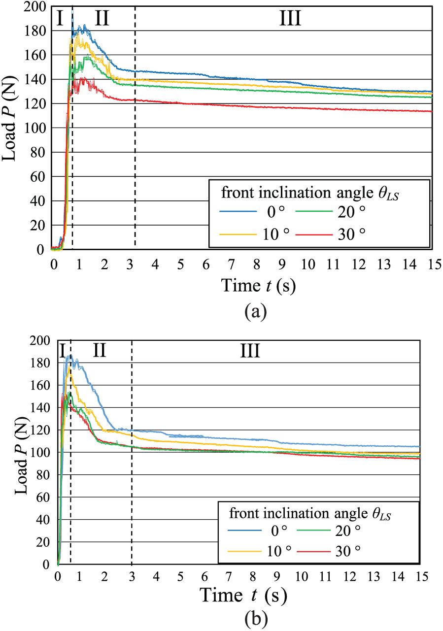
Relationship between load and time: (a) debris flow and (b) woody debris flow.

Figure 17.

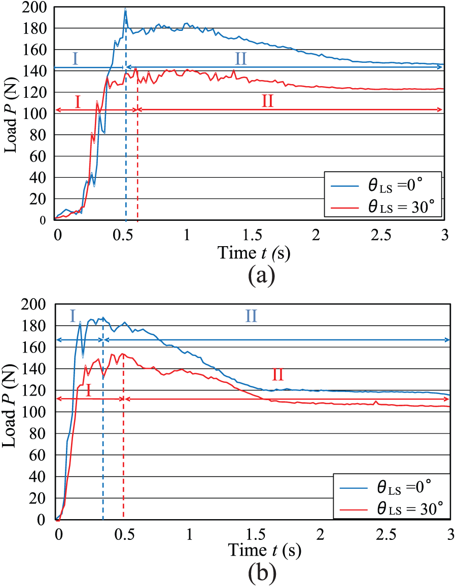
Relationship between load and time (define I and II as in Figure. 16): (a) debris flow and (b) woody debris flow.

Figure 18.

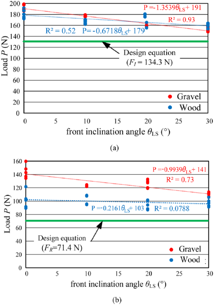
Maximum impact load and sedimentation load: (a) maximum impact load and (b) sedimentation load.

It was assumed the simple function to make it to the simplification for the comparison with the design. The purpose of this is to show that the collision load changes at the angle of the dam. Even if the shape of the Sabo dam changes, the design is evaluated as the same.

For the collision shown in blue of Figure 17, the maximum impact load for θ_LS = 0° is 186 N and that for θ_LS = 30° is 153 N

P_{I - G w} = - 0.672 θ_{L S} + 179

(2)

where P_I-Gw is the maximum impact load of woody debris flow. Here, the coefficient of determination (R²) is 0.52.

The results in Table 3 show that the generation time of the maximum load is less in debris flow than in woody debris flow. In the actual experiment, the surge of the debris flow mixed with wood normalizes. However, the maximum collision load does not decrease significantly when wood and debris are mixed. In other words, the collision load of the gravel usually placed between the driftwood reduced according to the front configuration of the debris flow. Figure 18(b) shows a red and blue point in case of sedimentation load. The sedimentation load for debris flow and woody debris flow, respectively, is given as follows

P_{I - G} = - 0.994 θ_{L S} + 141

(3)

P_{I - G w} = - 0.216 θ_{L S} + 103

(4)

where P_R-G is the sedimentation load of debris flow and P_R-Gw is the sedimentation load of woody debris flow.

The sedimentation load at θ_LS = 0 ° is 141 N, and that at θ_LS = 30° is 111 N, which is approximately 15% smaller. However, when the flow involves driftwood, the load at θ_LS = 0° is 103 N, and that at θ_LS = 30° is 90 N, which is approximately13% smaller. However, the number of experiment is little, and there is still room to examine that.

Comparison of Japanese design against debris flow

In the Sabo dam structure design handbook (National Institution for Land and Infrastructure Management, Ministry of Land, Infrastructure, Transport and Tourism, 2018), an open Sabo dam evaluates normally the debris of flow fluid force. The design formula is given as follows

F I = C_{d} \frac{ρ_{d}}{g} h B U^{2}

(5)

where F_I: fluid force, ，B: width of the action load, ρ_d: unit volume weight of the fluid, g: gravity, C_d: coefficient (C_d = 1.0), h: depth of debris flow, U: average fluid velocity of debris flow. The following values are substituted in this equation: B = 0.30 m, ρ_d = 25.4 kN/m³, g = 9.8 m/s², h = 0.12 m, and U = 1.2 m/s. Here, the velocity of debris flow was measured from the image of movie.

Therefore, F_I = 134.3 N, this value is indicated to Figure 18(a). The green line of design equation (F_I = 134.3 N) is smaller than experimental result of maximum impact load (Figure 18(a)).

The evaluation of the soil load is omitted in the design of open Sabo dam. However, the soil load formula in present design is given as follows

F R = \frac{1}{2} K_{a} B ρ_{S} {g h}_{2}^{2}

(6)

where K_a: coefficient of active earth pressure and h₂: height of the sedimentation. The following values are substituted in this equation: K_a = 0.3(design value), B = 0.30 m, ρ_Sg = 25.4 kN/m³, and h₂ = 0.25 cm. Therefore, F_R = 71.4 N, this value is indicated to Figure 18(b). The green line of design equation (F_R = 71.4 N) is smaller than experimental result of maximum impact load (Figure 18(b)).

Figure 18 shows the maximum impact loads, and the sedimentation load is approximately 1.5 times that of the design value.

Influence of inclination angle and capturing process on maximum impact load

The outcome of the experiment is summarized, and Figure 19 illustrates the mechanisms of debris flow to reduce impact load. First, the debris flow reaches the dam as shown in Figure 19(a)(I) and (b)(I). Figure 19(a)(II) indicates that half the height of the dam is under contact with the front side of the debris flow. This first contact surface reachs half of dam’s height in case of vertical dam. At this time, the mass of gravel is generally divided into two groups. The first group precedes and reaches the dam. The second group moves over the mass of gravel of the first group.

Figure 19.

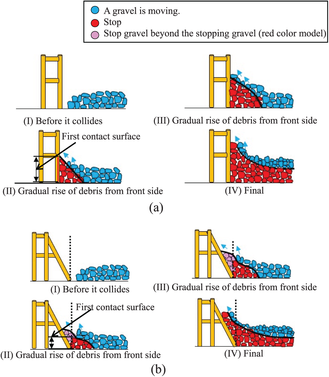
Difference of granular mechanism influence on front inclination angle: (a) vertical dam (e.g. θ_LS = 0°): (I) before it collides, (II) gradual rise of debris from front, (III) gradual rise of debris from front side, and (IV) final and (b) front inclination dam (e.g. θ_LS = 30°): (I) before it collides, (II) gradual rise of debris from, (III) gradual rise of debris from front side, and (IV) final.

Comparing the gravel of the following groups in Figure 7(a) and (b), the height of the sedimentation shape differed from each front inclination angles.

The following gravel easily reaches the vicinity of the Sabo dam and affects the front inclination. The inclination in front of the dam exists and, the amount of sedimentation in the dam increases. The process of sedimentation in front of the dam is shown as from Figure 19(b)(II)–(IV). In addition, an increase in the load ends at this point as shown in Figures 12 –15 and Figure 16. Moreover, the large inclination angle model becomes convex shaped, and it is arranged in the area shown by dashed lines in Figure 19(b)(III).

Subsequently, the length of the friction side of the gravel under the movement and the stopping gravel increases, and the collision load is decreased.

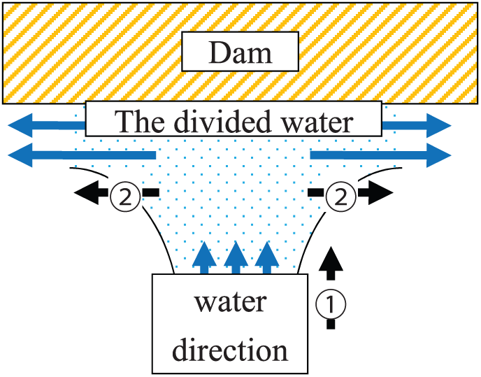
Figure 20 illustrates the debris flow load in the study by Daido et al. (1992). Although this is a horizontal chart, it dose not travel straight after the debris flow collide. Therefore, it is assumed to have changed the traveling direction to the orthogonal direction. The assumption proposes to lose all momentum in dividing into the two directions. In other words, the conversion of the traveling direction is diagonally pressed although vertical and horizontal differences exist. Therefore, the impact load can be reduced by decreasing the velocity of debris flow. The gravel that reaches previously stops the following debris flow by utilizing the front inclination angle of Sabo dam and this situation loses the velocity of debris flow. In addition, the front inclination angle of Sabo dam have a mechanism to decrease load, and this causes a delay of the maximum load generation time.

Figure 20.

Expression of design model (Daido et al., 1992; National Institution for Land and Infrastructure Management, Ministry of Land, Infrastructure, Transport and Tourism, 2018).

Conclusion

This study presents the relationship between load and time to evaluate the impact load of debris flow against a steel pipe open Sabo dam. In addition, the mechanism of the impact force was examined. In that case, the front inclination angle on the side of the dam influenced the decrease in the impact force.

The maximum impact load of front inclination angle (θ_LS = 30°) against debris flow is decreased in comparison with that of the impact load of front inclination angle (θ_LS = 0°). The impact load shows a decrease of approximately 30%.

In the case of woody debris flow, the maximum impact load in the largest front inclination angle (θ_LS = 30°) is decreased by approximately 20% in comparison with that of the smallest one (θ_LS = 0°).

In the case of a front inclination angle in the dam, the amount of the gravels and woody debris flow approaching the collision side decreases in comparison with the dam with no inclination (θ_LS = 0°).

The effect of driftwood of debris flow is able to decrease the maximum impact load in the experiment.

In future research, it is necessary to examine the decrease in impact load and trapping mechanism under the influence of the front inclination angle. In addition, comparing debris flow load in experiment and in the present design, it is important to examine reflection of the present design.

Footnotes

Declaration of conflicting interests

The author(s) declared no potential conflicts of interest with respect to the research, authorship, and/or publication of this article.

Funding

The author(s) received no financial support for the research, authorship, and/or publication of this article.

References

Adachi

(1964) Experimental study on artificial roughness. Transactions of the Japan Society of Civil Engineers 104: 33–44.

Beppu

Inoue

Ishikawa

et al . (2011) Numerical simulation of debris flow model by using modified MPS method with solid and liquid particles. Journal of Erosion Control Engineering 63(6): 32–42.

Daido

Yoshizumi

Nakajima

(1992) Impact force of mud-debris flows acting on structure. Proceeding of Hydraulic Engineering 38: 557–562.

Hiramatsu

Fukuyama

Yamada

et al . (2014) Disaster report on the debris flow occurred on 9 July 2014 in Nagiso, Nagano prefecture. Journal of Erosion Control Engineering 67(3): 38–48.

Ikeya

(1978) Classification of debris flow. Civil Engineering Journal 20(3): 44–49.

Iwamoto

Hirano

(1982) A study on the mechanism of the occurrence of debris flow and its flow characteristics. Journal of the Japanese Forestry Society 64(2): 48–55.

Miyoshi

Suzuki

(1990) Experimental study on impact load on a dam due to debris flow. Journal of Erosion Control Engineering 43(2): 11–19.

Mizuyama

(1979) The problem of debris flow impact force evaluation. Journal of Erosion Control Engineering 112: 40–43.

Mizuyama

Geto

Nakanishi

et al . (1985) Experimental study of the impact force of debris flow to a sabo dam made of steel pipes. Journal of Erosion Control Engineering 37(5): 30–34.

10.

Mizuyama

Kobashi

Mizuno

(1995) Control of passing sediment with grid-type dams. Journal of the Japan Society of Erosion Control Engineering 47(5): 8–13 (in Japanese).

11.

National Institution for Land and Infrastructure Management, Ministry of Land, Infrastructure, Transport and Tourism (2016) The Disaster Report of 16th Typhoon in 2016. Yokosuka, Japan: National Institution for Land and Infrastructure Management, Ministry of Land, Infrastructure, Transport and Tourism.

12.

National Institution for Land and Infrastructure Management, Ministry of Land, Infrastructure, Transport and Tourism (2017) The Disaster Report of Torrential Rain and Typhoon in Northern of Kyushu Area in 2017. Yokosuka, Japan: National Institution for Land and Infrastructure Management, Ministry of Land, Infrastructure, Transport and Tourism.

13.

National Institution for Land and Infrastructure Management, Ministry of Land, Infrastructure, Transport and Tourism (2018) Manual of Technical Standard for Establishing Sabo Master Plan for Debris Flow and Driftwood (no.904). Yokosuka, Japan: National Institution for Land and Infrastructure Management, Ministry of Land, Infrastructure, Transport and Tourism.

14.

Shibuya

Katsuki

Kokuryo

et al . (2012) Experimental study of load for steel frame check dam caused by debris flow with woody debris. Journal of Erosion Control Engineering 65(1): 54–61.

15.

Shima

Yoshida

Kawakami

et al . (2014) Consideration on boulders & members’ interval open type steel Sabo dam for capturing debris flow. Journal of Erosion Control Engineering 67(5): 3–11.

16.

Wada

Furutani

Nakatani

et al . (2015) Experimental study of factors that affect the concentration of larger particles at the front of debris flows. Journal of Erosion Control Engineering 67(6): 56–63.

17.

Watanabe

Mizuyama

Uehara

(1980) Fundamental examination of countermeasure of debris flow. Japan Society of Erosion Control Engineering 32(4): 40–45.

18.

Yamamoto

Toriihara

et al . (1998) Impact load on Sabo dam due to debris flow. Journal of Erosion Control Engineering 51(2): 22–30.