A Primer on Inverse Probability of Treatment Weighting and Marginal Structural Models

Abstract

Emerging adulthood researchers are often interested in the effects of developmental tasks. The majority of transitions that occur during the period of early/emerging adulthood are not randomized; therefore, their effects on developmental trajectories are subject to potential bias due to confounding. Traditionally, confounding has been addressed using regression adjustment; however, there are viable alternatives, such as propensity score matching and inverse probability of treatment weighting. Propensity scores are probabilities of selecting treatment given values on observed covariates. Inverse probability of treatment weights are also based on estimated probabilities of treatment selection and can be used to create so-called pseudo-populations in which confounders and treatment are unrelated to each other. In longitudinal models, such weighting can occur at multiple time points. This article provides a primer on these weighting methods and illustrates their application to studies of emerging adulthood. We provide annotated computer code for both SPSS and R, for both binary and continuous treatments.

Keywords

propensity scores inverse probability of treatment weights (IPTWs)marginal structural models (MSMs)confounding causal inference

Emerging adulthood researchers are often interested in developmental milestones that emerge during specific periods in the life of young adults. For example, Jonkmann, Thoemmes, Lüdtke, and Trautwein (2014) examined the effects of leaving the home on personality development in a sample of emerging adults. Leaving the parental home is clearly a nonrandomized event that is influenced by various observed or unobserved variables, and the authors discussed issues of confounding and tried to address it using various techniques, including propensity score matching. Another example is a study by Jackson, Thoemmes, Jonkmann, Lüdtke, and Trautwein (2012) that examined emerging adults who either entered military or civil service, and how this affected their personality development. Entrance into military service was again a nonrandomized event, and the study attempted to account for confounding through the use of regression adjustment and propensity scores in conjunction with latent growth models.

Both of these examples illustrate the ways in which observed changes in developmental trajectories are influenced by intervention, self-selection, or life events that are not randomized. It is well known that effects observed in nonrandomized studies are subject to bias due to confounding (e.g., Cochran & Rubin, 1973; Greenland, Pearl, & Robins, 1999; Greenland & Robins, 1986). Generally speaking, variables that have an effect on both the treatment selection and the outcome are known as confounders. Given that arguably many studies of emerging adulthood deal with effects of nonrandomized treatments, it is an important question as to how an applied researcher should address the problem of bias due to confounders.

Adjustment for Confounding

Traditionally, researchers in the social sciences have predominantly used regression adjustment to control for observed confounders. This typically amounts to estimating an analysis of covariance model, or more generally a multiple regression model in which the effect of interest (or the putative cause) is represented by a predictor or set of predictor variables, alongside a potentially larger number of covariates. In research in the social sciences, it is customary to include only linear terms of covariates that are not expected to be influenced by the treatment (e.g., mediators; Rosenbaum, 1984). This type of regression adjustment is ubiquitous in both cross-sectional and longitudinal investigations to a degree that thinking about “adjustment” or “control” is often synonymous with the act of adding another variable in a regression model. Adjustment through regression is theoretically sound practice, but it is not without criticism (e.g., Berk, 2004; Schafer & Kang, 2008).

A key criticism of regression adjustment is that researchers typically rely on a linear functional form between the covariate and the outcome. This linearity assumption is often untested, especially in the presence of a large number of covariates. It is possible to test for nonlinear effects, for example, through examination of scatterplots, or so-called added-variable plots (Cook & Weisberg, 2009), but it becomes exceedingly difficult to also rule out any interactive effects between the covariates and the putative cause, thereby making regression adjustment potentially more dependent on modeling choices (i.e., results may differ depending on whether a linear or different type of model is chosen for adjustment). The problems that arise when relationships between covariates and outcomes are nonlinear and incorrect linear models are used for adjustment are discussed by Rubin (1979) or more recently by Gutman and Rubin (2015). These authors argue that under departures from linearity, the classic regression adjustment fails to remove bias and can in fact increase biases in treatment effect estimates, if a misspecified model (e.g., a linear model) is used for adjustment.

Additionally, in regression adjustment, it is very difficult for researchers to know whether the adjusted effect is based on extrapolation. If the (multivariate) covariate distributions of participants in different treatment conditions are very different from each other, then overlap in multidimensional space might be sparse. In other words, there are no treated participants who are similar or comparable to any of the untreated participants on the totality of the observed covariates, and any comparison between the two groups might be due to extrapolation (King & Zeng, 2006).

Finally, as others have noted (Rubin, 2001), the ease with which regression models with different numbers of covariates can be estimated and evaluated may introduce biases through cherry-picking models that produce desired outcomes. This criticism is not aimed at the method of regression per se, but rather at the way it is potentially applied in practice.

Inverse Probability of Treatment Weighting

An alternative to regression adjustment is to utilize so-called inverse probability of treatment weights (IPTWs) to account for biases due to observed confounders. IPTWs are currently not widely used in psychology but are more frequently seen in epidemiological research. IPTWs share some features with propensity scores (Rosenbaum & Rubin, 1983b). We will use the propensity score as a springboard for our introduction to IPTW but will not discuss propensity score matching strategies in much detail, as there are a large number of well-written introductory pieces (Austin, 2011; Caliendo & Kopeinig, 2008; D’Agostino, 1998; Dehejia & Wahba, 2002; Luellen, Shadish, & Clark, 2005; Stuart, 2010), in addition to papers that have reviewed the literature on best practices (Austin, 2008; Thoemmes & Kim, 2011) or contrasted matching with more traditional approaches (West & Thoemmes, 2008). Many of the introductory papers on this topic also include expositions on the so-called potential outcomes model. Readers interested in the formal definition of causal effects using potential outcomes are referred to Rubin (2005).

The fact that we are using the propensity score to introduce IPTW should not give the impression that IPTW originated from the propensity score literature. On the contrary, they were developed independently by Robins (1986) in a paper that has been described as “revolutionary” (Vansteelandt & Daniel, 2014, p. 740). Our own discussion of IPTW and their use benefited greatly from several papers that explained this method previously (Bray, Almirall, Zimmerman, Lynam, & Murphy, 2006; Coffman & Zhong, 2012; Daniel, Cousens, De Stavola, Kenward, & Sterne, 2013; Daniel, De Stavola, & Cousens, 2011; Hogan & Lancaster, 2004; Robins, Hernán, & Brumback, 2000).

The propensity score is a conditional probability of being assigned (or selecting) a treatment condition, given an observed set of covariates. This is formally expressed as e(x) = P(Z = 1|X), where Z is a binary treatment indicator and X is a vector of observed covariates. We should add that this vector X must contain all confounders (a condition sometimes called ignorability, Rosenbaum & Rubin, 1983b, or more colloquially the assumption of no unmeasured confounders) to remove confounding bias completely. If unobserved confounders are present, ignorability does not hold, and residual bias can remain no matter which method (regression adjustment, propensity score matching, and IPTW) is used.

The fundamental difference between regression adjustment and approaches using propensity scores (which includes IPTW) is that the former models the relationship between a covariate and the outcome, whereas the latter models the relationship between the covariate and the putative cause (i.e., treatment assignment). In the case of matching, the propensity score is used directly to form matches within a data set. Under some matching schemes, this can result in some participants being discarded. The retained participants are expected to be well matched and exhibit balance on the covariates, a property that would also be expected under randomization. Balanced covariates cannot be confounders anymore (as they are unrelated to treatment assignment), and it is through this balance property that propensity score matching addresses issues of bias due to observed confounders. IPTW on the other hand uses the propensity score to form a weight. Weighting is a strategy that has long been used in survey sampling (Horvitz & Thompson, 1952). IPTWs are used to create a pseudo-population in which the covariates and the treatment assignment are independent of each other (a property that we would expect under randomization). The term pseudo-population reflects the fact that the weighted groups are not identical to the population that was actually observed but that this weighted group could have been sampled from a population in which there was no confounding. Such an approach may seem strange at first, after all we are creating weighted groups that did not exist in this way when we sampled our participants. At worst, it seems like that we are cheating and are not using the actually observed data, but some idealized form of it. However, as it turns out, both regression adjustment and propensity score matching can be conceptualized as types of weighting. Consider first, propensity score matching in which, due to a particular matching scheme, some participants are matched and others are discarded. This can be recast as a simple weighting scheme in which each matched participant receives a weight of 1 and each unmatched participant receives a weight of 0. We should add that dropping participants in propensity score matching is neither guaranteed to happen (some matching schemes retain more or all units) nor necessarily a bad thing (because dropped participants are usually so dissimilar from other individuals that causal comparisons would be a moot point). Angrist and Pischke (2008) explain in a very detailed and mathematically rigorous way that regression is also a special weighted matching scheme. In that sense, regression adjustment, matching, and weighting are all in the same class of methods.

How are the IPTWs formed? In the simplest case of IPTW in which we have a single treatment with two conditions observed one single time, we construct the IPTWs by estimating each person’s probability of having received their respective treatment, based on the observed covariates, and then weight by the inverse of this estimated probability. That is, participants in the treatment condition receive a weight of 1/P(Z = 1|X), and participants in the control condition receive a weight of 1/(1 − P(Z = 1|X)). These weights are also referred to as unstabilized weights. Note that the denominator term for the treated subject is identical to the propensity score. The denominator terms of the weights are often derived from a logistic regression model, in which the treatment selection is being predicted by the observed covariates. However, other models (e.g., regression trees and boosting algorithms, Zhu, Coffman, & Ghosh, 2015, or other data mining approaches) are possible. The so-called unstabilized weights can have the disadvantage that large weights can emerge. For example, a participant who is highly unlikely to select the treatment (based on the observed covariates) and ends up taking the treatment will get a very large weight. Analyses will thus become heavily dependent on a single or few individuals. This often increases the variance (and hence the associated uncertainty of estimates), sometimes dramatically so. To counter these ill effects, one may use so-called stabilized weights. As a general rule, stabilized weights should always be preferred over regular weights (Hernán, Brumback, & Robins, 2000; Robins et al., 2000). Stabilized weights only differ from the weights described above in that they do not take a simple inverse but instead divide the baseline probability of selecting a treatment (estimated from a model with no covariates) by the probability of selecting treatment given the covariates. In other words, in cases of binary treatments, the numerator of the unstabilized weights, which is 1, is replaced by the proportion of participants who selected the treatment. Thus, the weights are P(Z = 1)/P(Z = 1|X) for treated participants and 1 − P(Z = 1)/(1 − P(Z = 1|X)) for participants in the control condition. Stabilized weights tend to produce estimates that have smaller variance.

An additional strategy to deal with large weights is to set them to a less extreme value (e.g., by recoding all weights that are outside the 5th and 95th percentiles). Cole and Hernán (2008) refer to this as truncation or trimming. In other fields, this is also known as winsorizing. Truncation may be done after stabilizing the weights.

So far we have only considered weights for binary treatments, but an advantage of weights is that they easily generalize and can be constructed for nonbinary treatments, including continuous variables that are assumed to be putative causes. Instead of estimating predicted probabilities of group membership, conditional densities are used. This is typically achieved by fitting a (linear) regression model that predicts the continuous putative cause based on a set of covariates and then obtaining the conditional density of the predicted value for each person based on a normal probability density function. Denoting the normal probability density function as ϕ, and the expectation operator as E, we may denote the stabilized weights for a continuous putative cause as φ(E(Z))/φ(E(Z|X)). While this formula appears a little more daunting, it can be easily broken down into comprehensible pieces. To obtain the numerator, we run a regression without any predictors in which the outcome is the continuous cause. This regression therefore only includes the intercept. The predicted values of this regression are constant, and they are all simply the mean of the continuous variable. We then compute for each single individual value of the continuous cause the conditional density based on a normal distribution with mean equal to the intercept and standard deviation equal to the standard deviation of the residuals of this regression. This is the numerator of the weight. To obtain the denominator, we run a regression in which we use all covariates that we have selected as confounders to predict the continuous treatment in a linear regression model. We again derive conditional densities for each individual based on their observed value on the continuous cause based on a normal distribution with mean equal to the predicted value of the regression mentioned above and standard deviation equal to the residuals of the standard deviation of this same regression. This is the denominator of the weight. The final weight is the ratio of numerator and denominator. As explained in more detail in Robins, Hernán, and Brumback (2000), weights for continuous variables always need to be stabilized. Coffman and Zhong (2012) provide a great introduction with easily accessible formulas along with detailed computer code to estimate weights in the case of continuous putative causes.

Once IPTWs are obtained, treatment effects are estimated using whichever outcome model was desired (e.g., a regression model), by incorporating the weights, for example, in a weighted regression. Performing this type of weighted regression on the data is conceptually identical to running an unweighted, regular regression model in the pseudo-population in which confounders and treatment are independent of each other. One complication is that the weights themselves are also estimated and thus have sampling variability. To account for the uncertainty that the weights are not fixed but were estimated from data, it is common to use robust sandwich standard errors (Huber, 1967; White, 1980). Alternately, one may bootstrap the standard errors (i.e., empirically approximate a sampling distribution through repeated sampling) and form confidence intervals (or hypothesis tests) based on the bootstrap distribution.

The success of using weighting to control for bias due to confounding rests on several assumptions, some of them untestable, others at least in theory refutable. The following key assumptions must be met (Cole & Hernán, 2008):

No unmeasured confounding: We have already mentioned the ignorability assumption, which essentially is an assumption that there are no unobserved confounders. This assumption is critical and unfortunately not testable. It is an assumption that is shared by all methods that try to adjust on observed confounders. It is immediately apparent that such an assumption is untestable, because if a confounder has not been observed, its potentially biasing effect on the estimate cannot be computed. Researchers are thus encouraged to make a theoretical argument as to why they believe that they have collected all important confounders. Some authors (Pearl, 2009; Sjölander, 2009) recommend the use of a causal graph to help researchers think about which variables are potential confounders and should, therefore, be controlled in analyses. In addition, a so-called sensitivity analysis (Rosenbaum & Rubin, 1983a; VanderWeele, 2008; VanderWeele & Arah, 2011) can bolster faith that even in the presence of an unmeasured confounder, the results would not change dramatically. In a sensitivity analysis, the researcher makes certain assumptions about the magnitude of the unobserved confounder and then computes how much the effect would change if such a confounder was present. If the effect does not change much, even in the presence of a strong confounder, we have increased faith that our results are robust against unmeasured confounders.

Positivity: The positivity assumption states that every unit must have at least a nonzero probability to receive either treatment. Statistically speaking, it means that none of the predicted values that are used to compute the propensity score (and thus the IPTW) can be 0 or 1. This would happen every time when there are participants with certain values on the covariates that were all assigned to the treatment or all assigned to the control condition. Note that with continuous variables, or in general with many covariates, this is very likely to happen, because continuous variables have by definition an infinite number of values that they can take on, even though in practice those are not all observed. When this occurs, researchers can either simply discard these participants with the understanding that a causal effect would be undefined for the discarded subjects—after all, there are simply no participants with these particular covariate combinations that were observed in both treatment and control, thus any causal effect estimate would necessarily be based on extrapolation. This is especially defensible when the excluded participants can be reasonably argued to be an unusual subset of participants. Describing these excluded participants may also be informative to explore the generalizability of the results (Stuart, Cole, Bradshaw, & Leaf, 2011). However, this argument for exclusion may not always be convincing, for example, when there are participants who would have to be excluded simply because they take on a unique (but otherwise comparable) value on a continuous covariate. An alternative in such a case is to use a parametric model (e.g., a logistic regression) when estimating the propensity score to smooth over these cases. The use of parametric models may mask violations of positivity to an applied researcher, and thus positivity checks in conjunction with the estimation are recommended. One possible check is the examination of cross-tables to see whether each combination of covariate values contains both treated and untreated participants. This becomes cumbersome with many covariates, and an alternative is to inspect the so-called convex hull (Iacus, King, & Porro, 2011; King & Zeng, 2006), which is a method that specifically constructs areas of multidimensional overlap and informs the researcher of all participants in one group that fall outside an observed range on all covariates of participants of the other group.

Correct specification of the IPTW: When estimating the IPTW, we often use a logistic regression to estimate the propensity score that is later used to form the weights. Although other methods are possible, the use of parametric models (such as logistic regression) is quite widespread. Any parametric model may be misspecified (e.g., omission of a nonlinear or interactive term). If such a misspecification occurs, the resulting propensity scores and the IPTWs will not remove all confounding bias. In some cases, residual bias may remain, or worse, misspecifications can increase bias. There are several strategies to address misspecification. One strategy is to form potentially fine-grained categories out of all continuous covariates, and then fit models that allow for interactions between the categorical variable. If all possible interactions are included, we refer to this as a saturated model. This strategy can help alleviate bias due to omitted nonlinearities but can result in highly parameterized models that are potentially much more variable. Another strategy is to use smoothing techniques, such as splines or general additive models that account for nonlinear relationships. Some researchers (van der Laan, Polley, & Hubbard, 2007) strongly prefer data mining techniques to break the reliance on parametric models (for a review, see McCaffrey, Ridgeway, & Morral, 2004; Lee, Lessler, & Stuart, 2010; Sekhon, 2011; Imai & Ratkovic, 2014; or Westreich, Lessler, & Jonsson Funk, 2010). Cole and Hernán (2008) suggest trying different estimations and truncations of weights and to check for each of the solutions whether the stabilized weights have a mean of 1.0 and a minimum and maximum that is not very extreme. While there are no cutoffs of what “extreme” means, weights that are in the hundreds or even higher can be considered quite large.

When Is This Method Applicable in Emerging Adulthood Research?

As outlined above, IPTW can be used to adjust for observed confounding, thereby making it applicable in any situation in which a nonrandomized treatment is being evaluated. IPTW can be used with binary treatments but also multinominal treatments or even continuous putative causes. In short, it can be used whenever regression adjustment is an option. Does that mean that IPTW should always be preferred over regression adjustment or propensity score matching? Not necessarily—in situations in which the assumptions of linear regression adjustment are fulfilled and a parametric functional form between covariates and outcome can be specified, it is possible that regression adjustment will perform just as well or better than IPTW. On the other hand, if the covariate–outcome relationship cannot be easily approximated with parametric models, but the relationship between covariates and treatment selection can, it might be preferable to use IPTW. An applied researcher might use both methods of adjustment in the hope that the two methods would agree on their respective conclusions. If so, this would bolster faith in the robustness toward model choice. If not, this may be a hint that one of the models is misspecified. One domain where IPTW is arguably superior over regression adjustment are problems with longitudinal data with time-varying confounders, and time-varying treatments, which we will discuss later.

Simulated, Numerical Example of IPTW With Treatments at Single Time Points

We now provide a numerical example using simulated data. Replication code for this example in R and SPSS is available in the Appendix and can be downloaded at http://www.human.cornell.edu/hd/qml/replication-code.cfm. The example is purposefully kept as simple as possible to highlight the underlying mechanisms. Consider first a single binary putative cause X, for example, treatment versus control, a continuous outcome Y, for example, the level of depression at posttest, a single binary confounder C₁, for example, the presence or absence of a risk factor, such as drug abuse, and a single continuous confounder C₂, for example, the level of anxiety measured before treatment administration. We are interested in the effect of the treatment on depression, but the treatment is not randomized, and participants with and without a history of drug abuse, and different levels of anxiety, are selectively choosing the treatment. Both covariates are also affecting depression at posttest, thus making them confounders. We simulated a data set of 2,000 participants (sample size was set high to avoid results that are unduly influenced by the particular random sampling) in which this confounding structure was present, and the true causal treatment effect was 0.1 on an unstandardized metric. However, participants with a history of drug abuse were less likely to select the treatment, and drug abuse had a positive effect on depression (increasing depression), thus biasing the relationship. Likewise, participants who were more anxious were less likely to take the treatment and also had increased depression at posttest, again biasing the relationship. An unadjusted effect (i.e., computing a t-test of the difference on the outcome using just treatment assignment) yielded an effect of .03, with a standard error (SE) of .026, suggesting a very small or no (statistically significant) effect of the treatment. We then estimated the stabilized and truncated weights (with truncation at both 1% and 5% most extreme scores), using the formulas mentioned above. Results for all three weighting schemes and for regular regression adjustment (for comparative purposes) are reported in Table 1.

Table 1.

Results of the Simulated Example With Treatment Effects at One Point in Time.

Method	Mean Weight	Min/Max Weight	Estimated Effect (SE)
True effect	—	—	.10
Unadjusted	—	—	.03 (.026)
Regression	—	—	.11 (.022)
Stabilized IPTW	1.000	0.75, 1.49	.11 (.026)
Stabilized IPTW, 1% truncated	0.999	0.78, 1.34	.11 (.026)
Stabilized IPTW, 5% truncated	0.999	0.80, 1.30	.11 (.026)

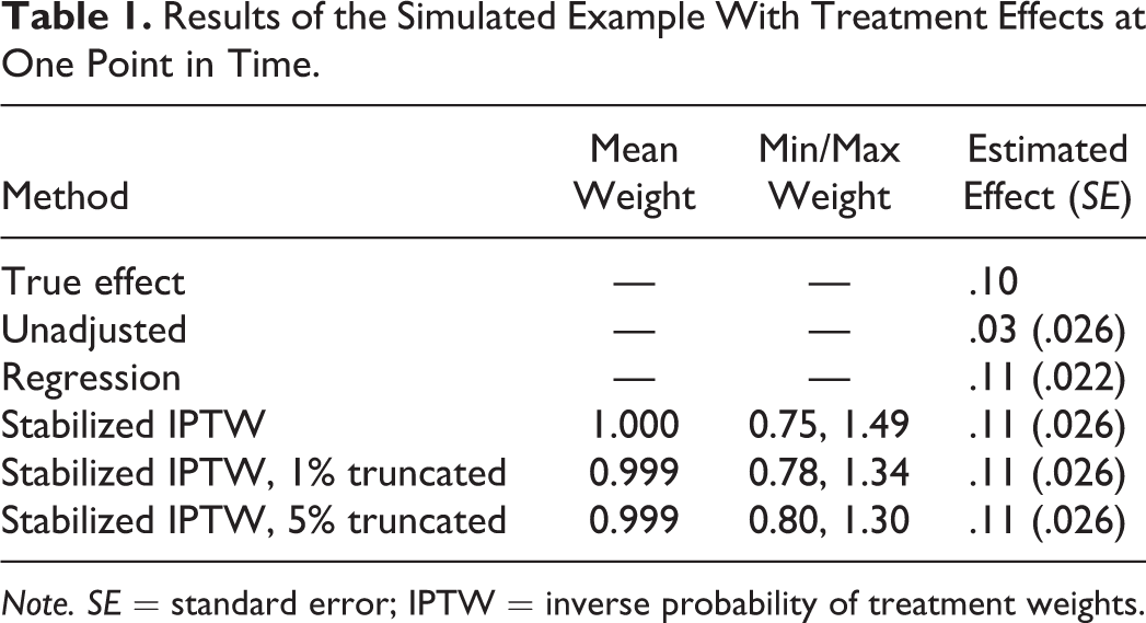
Note. SE = standard error; IPTW = inverse probability of treatment weights.

We observe that all methods (including regression) perform quite well in this scenario. The unbiased effect of .10 is essentially recovered by all methods. In fact, the differences in both estimates and standard error are absolutely minimal. Given that this was a very simple example (two confounders, only linear relationships), this was expected. We further observe that all weights were approximately centered on 1, indicating that there was no misspecification in the weights. Lastly, we observe that results from regression and weighting with and without truncation were quite similar. It is important to repeat that this was an idealized situation, and actual data analysis will not necessarily yield results that align so closely with each other (see however Cole & Hernán, 2008, for a real example in which results are also quite consistent across different specifications). In addition to the effect estimate, it is informative to look at differences on the covariates between treatment conditions before and after weighting. Before weighting, the covariates differed quite a bit in their propensity to either take the treatment or not. The differences on the binary covariate in the percentage of participants taking the treatment were about 20%, and for the continuous covariate, this difference was 5% for each unit increase in the covariate. After weighting, the difference was 0% for both covariates—an expected result under a correctly specified weighting model. This highlights again the property of IPTW to create pseudo-populations in which confounders and treatment assignment are independent of each other.

Extending the Method to Longitudinal Data

Emerging adulthood researchers are almost always interested in estimating effects that span more than one time point. An added complication of this type of research is that participants may move in and out of a treatment. For example, Jonkmann et al. (2014) investigated the effect of changes in living situations on personality development in young adults. Some of the young adults changed their living arrangement during the 3 years of data collection.

In addition, confounders of relevant relationships may be time variant, meaning that they take on different values at different points in time, and confounders at later points in time may be affected by previous confounders, previous treatment assignments, or previous outcome variables. This entangled structure in longitudinal data makes it impossible to use regression adjustment to estimate certain types of effect (Robins, 1986). Specifically, conditioning on variables that are confounders for later outcomes (as would be done in regression with longitudinal data), but are at the same time also caused by earlier treatment variables, has the potential to increase bias for two reasons. First, any variables whose causal effect was of interest that had an effect on one of the covariates that we conditioned on will incur bias because a causal pathway of this variable is now blocked (sometimes referred to as overadjustment). Second, unobserved covariates (even if they were not confounders) that have an effect on the variable that we conditioned on in the regression, and also have an effect on other variables of interest in our model, will now bias effects of interest (sometimes referred to as endogenous selection or collider bias). This type of collider bias has been explored in the causal inference literature (Cole et al., 2010; Greenland, 2003) and recently also in the missing data literature (Mohan, Pearl, & Tian, 2013; Thoemmes & Mohan, 2015; Thoemmes & Rose, 2014).

Likewise, the use of propensity score matching is infeasible if the treatment itself is time varying because this would involve repeatedly matching at every time point, potentially with different participants, making it impossible to actually describe longitudinal change. There is in fact currently no implementation for propensity score matching for longitudinal data with time-varying treatments.

To illustrate the type of data situations that we would encounter in such a setting, consider a study designed to investigate the effects of a hypothetical intervention to reduce subsequent levels of depression over time (e.g., VanderWeele, Hawkley, Thisted, & Cacioppo, 2011). Consider further that the intervention is offered over 3 years, and data are collected longitudinally for a total of 4 years that includes a year of posttest data. The decision to participate in the program is not randomized, meaning that participants can self-select at any time in the program. Because of this nonrandomized self-selection into the treatment, we may assume that existing personality traits, prior depression (and many other covariates) are potential confounders for the treatment effect on depression. In addition to depression levels, we measure a potentially large array of confounding variables across all time points. These covariates, just like the outcome and treatment status, are time varying. In this particular data structure, several research questions of interest could be posed. A natural question might be to ask: What is the causal effect of the treatment at each time point on the outcome at the latest time point? Another question might be: What is the causal effect of any given particular sequence of being treated or untreated on the outcome, for example, what is the effect of being treated at every single time point versus only being treated at the first time point and then never again? A similar question might be what is the cumulative causal effect of being treated at various time points, for example, what is the effect of being treated at least once versus being treated at all times, or not at all? All of these questions can be reasonably asked, and they can be answered using IPTW and marginal structural models (MSMs).

MSMs are essentially a way to formulate causal research questions. An MSM describes the causal relationships of interest among the treatment and potential outcomes. An MSM may look on the surface like a regression model that relates certain treatment assignments over time to an outcome of interest; however, instead of considering the observed outcome, it considers the potential outcomes that could have been observed under different potential time-varying treatment regimes.

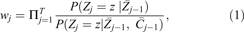
Earlier we established that IPWT can deconfound relationships by creating pseudo-populations in which confounders and treatment assignment are unrelated to each other. In the longitudinal case with time-varying variables, we will try to do the same thing. Specifically, we will weight in such a way that the time-varying treatment is independent of all stable and time-varying covariates that preceded it, at every time point. How are the weights formed that will achieve such independence of treatment assignment at every point and all preceding confounders? The way to form IPTWs in the time-varying case is to essentially repeat the process of weighting at every single time point. That means that at the first treatment occurrence, an initial set of weights is formed, just as outlined in the previous section (including potential stabilization and truncation), to make the treatment at the first time point independent of all covariates that preceded it. Just as previously, logistic regression (or other models) can be used to predict binary treatment selection at this time point, given the observed history of covariates. At the next time point, another set of weights are formed that make the treatment selection at Time 2 independent of all observed covariates that are causally prior to this treatment selection. Importantly, this includes the treatment selection at the previous time points. By repeating this step for all time points, each participant gets a weight for each time point. Once these weights are available, they are simply multiplied to form a single final weight. This weight is then used in whatever outcome model of interest (e.g., looking at the effect of the treatment at each time point, or looking at effects of particular treatment sequences, or looking at the effect of number of treatment occurrences over time, etc.). Of course, the selection of the covariates that ensure an unbiased effect is potentially even more difficult, as more treatments and more potential confounders over time need to be considered. And just like in the previous section, the weights should be stabilized, inspected, and then potentially truncated, if extreme weights are present. A minor wrinkle in the estimation and stabilization of these weights is that the numerator of weights of later time points (which used to be the predicted value of treatment assignment) is now chosen to be the predicted value of treatment assignment, given the complete treatment history of each person (Robins et al., 2000). Taking all this together, we end up with a definition of the weights in longitudinal settings for binary treatments as follows, following the notation of Bray, Almirall, Zimmerman, Lynam, and Murphy (2006):

w_{j} = Π_{j = 1}^{T} \frac{P (Z_{j} = z | {\bar{Z}}_{j - 1})}{P (Z_{j} = z | {\bar{Z}}_{j - 1}, {\bar{C}}_{j - 1})},

where w is the weight, j an index of time ranging from j = 1 to T, Z a binary treatment indicator, taking on values z,

{\bar{Z}}_{j - 1}

, is the history of the participant on previous treatment variables Z that occurred at all previous times up until j − 1, meaning all time points up until the one that is currently being weighted, and finally

{\bar{C}}_{j - 1}

is the set of time-varying or constant (baseline) confounders up until the time point j − 1. Weights for continuous treatments would be formulated as a similar extension of the weights for continuous treatments at a single point, described in the previous section. We will present weights for continuous treatments in longitudinal settings in the later example.

When Is This Method Applicable in Emerging Adulthood Research?

Whenever nonrandomized treatments (and covariates and outcomes) are time varying, MSMs with IPTW can be usefully applied. That is, any time it is of interest to examine how a nonrandomized treatment in a longitudinal setting has an effect on a posttest outcome variable, these models can be used. The resulting estimates inform researchers about the effects of being treated at each of the single time points. In addition, researchers can estimate cumulative effects, which often is relevant if a dose–response and/or continuing exposure to a treatment is expected.

Examples in emerging adulthood research are very sparse. VanderWeele, Hawkley, Thisted, and Cacioppo (2011) examined the link between depression and loneliness (both time varying) using these methods. Coffman and Zhong (2012) examined relationships between job training, job self-efficacy, and depression in the Job Search Intervention Study (JOBS II; Vinokur, Schul, Vuori, & Price, 2000). Bray et al. (2006) presented an illustrative example on the relationship between alcohol and marijuana initiation in young adults.

Simulated, Numerical Example of IPTW in Longitudinal Designs

To illustrate the technique, we again use a small simulated numerical example. The model of interest is shown in Figure 1 and is, despite its size, among the smallest possible models of a nonrandomized longitudinal study with time-varying confounding. A continuous treatment T is being observed at two time points, yielding TREAT₁ and TREAT₂. A continuous baseline covariate C confounds all relationships between all treatments, covariates, and outcomes. The outcome variable DEP is also measured 2 times. DEP₁ is therefore the pretest of the final outcome DEP₂. Further note that the pretests are confounding some of the later relationships, for example, DEP₁ is a confounder of the relationship between TREAT₂ and DEP₂.

Figure 1.

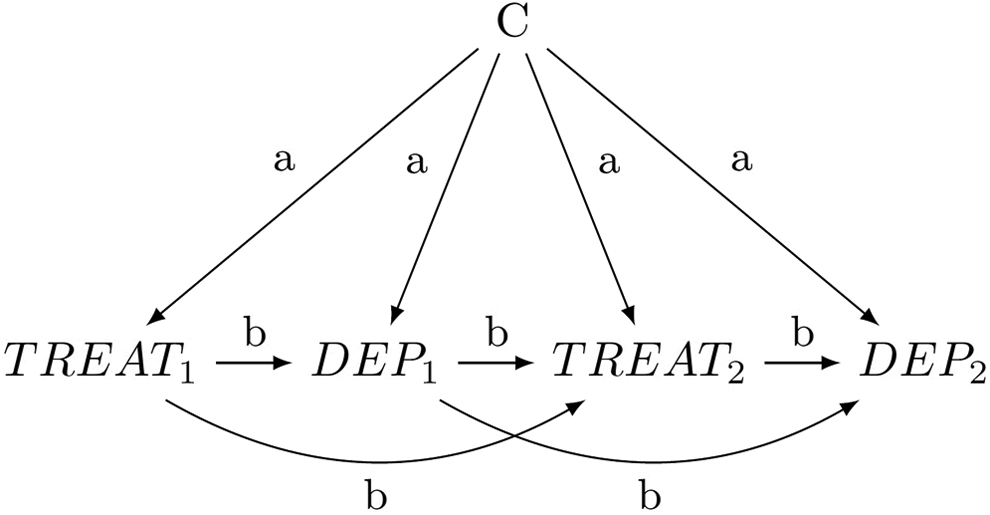
Assumed causal model for the numerical example of a model with time-varying treatments and covariates.

The labeled paths in Figure 1 are set to simple values in this example. The baseline confounder C always has a small effect of a = .1 on all other later variables. The direct effects of treatment (TREAT₁ and TREAT₂) on subsequent depression scores (DEP₁ and DEP₂) are all set to b = .4. Likewise, the path from intermediate depression DEP₁ to subsequent treatment TREAT₂ is also set to b = .4. The autoregressive effects among the variables DEP₁ and DEP₂ and the two treatments TREAT₁ and TREAT₂ are all set to b = .4. All variances of all continuous variables were set to 1, essentially standardizing them.

In this particular model, we may be interested in the joint effect of the treatments at various time points on our final outcome. If we could assume no confounding (which of course is incorrect in this model), we could fit a simple regression model predicting DEP₂ from both TREAT₁ and TREAT₂. This however will not work if confounding is present. Somewhat surprisingly, what will also not work is to estimate a regression model predicting DEP₂ from both TREAT₁ and TREAT₂ and all of the observed confounders, here C, DEP₁. The reason for this is that some of the variables, in particular DEP₁, are at the same time confounders (that need to be conditioned on) but also mediators of causal effects (here in particular the effect of TREAT₁ on DEP₂) and should therefore not be conditioned on. This general inability of regression models to properly adjust for confounding in time-varying contexts is well-documented (Bray et al., 2006; Robins et al., 2000). What does work though is to form weights that make both TREAT₁ and TREAT₂ independent of the confounders that preceded them. In this particular example, we would estimate the following weights for the continuous treatment variable TREAT₁:

w_{1} = \frac{φ(E ({TREAT}_{1} = t_{i}))}{φ(E {(TREAT}_{1} = t_{i} | C))},

where t is an indicator of the actual treatment that was received, either 0 or 1, and ϕ and E, the normal density and expectation operator, respectively. Note that this is simply a weight, just as we have used previously, that uses all variables in the weighting formula that occur prior to treatment at Time 1.

We will use the following weights for TREAT₂:

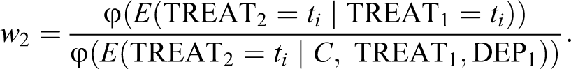
w_{2} = \frac{φ (E ({TREAT}_{2} = t_{i} | {TREAT}_{1} = t_{i}))}{φ (E ({TREAT}_{2} = t_{i} | C, {TREAT}_{1}, {DEP}_{1}))} .

Again, this is a weight that uses all variables that are causally prior to treatment at Time 2. Note that the numerator is now the conditional probability of receiving the respective treatment, given the actually observed treatment history. Here, the complete treatment history is simply the one previous measure TREAT₁. In general, the weights for later time points will always include all previous variables on the right of the conditioning bar in the denominator term, and all previous treatment assignments in the numerator term on the right of the conditioning bar. In general, this is how weights in longitudinal settings are always constructed. The product of these two weights, w ₁ × w ₂, is the final analysis weight.

Given the data-generating model in Figure 1, we can derive the true causal effects of TREAT₁ and TREAT₂ on DEP₂. The individual effects are .16 for TREAT₁ and .40 for TREAT₂. Table 2 reports the results of the numerical example using a large sample size of 2,000 (to minimize sampling variability). We report results of a regression model with no covariates and either TREAT₁ or TREAT₂ alone, a regression model with both treatment variables, but no covariates, and a model with both treatment variables and all covariates. Finally, we present results using IPTW, with stabilized weights, and with truncations of 1% and 5% of the most extreme weights. All outcome models were estimated using generalized estimating equations to account for the repeated measures structure. These models yield robust standard errors.

Table 2.

Results of the Simulated Example With Time-Varying Treatments.

Method	Mean Weight	Min/Max Weight	Estimated effect TREAT₁ (SE)	Estimated effect TREAT₂ (SE)
True effect	—	—	.140	.400
Regression with only TREAT₁	—	—	.423 (.022)	—
Regression with only TREAT₂	—	—	—	.574 (.017)
Regression with both treatments	—	—	.048 (.022)	.623 (.020)
Regression with both treatments and all covariates	—	—	.011 (.019)	.399 (.021)
Stabilized IPTW	.989	.03, 15.19	.157 (.031)	.421 (.036)
Stabilized IPTW, 1% truncated	.968	.18, 3.92	.154 (.026)	.433 (.026)
Stabilized IPTW, 5% truncated	.931	.39, 1.92	.131 (.024)	.480 (.023)

Note. SE = standard error; IPTW = inverse probability of treatment weights.

We observe that the true values of .16 and .40 for the two direct treatment effects are not recovered in any of the models without any adjustment. This includes the regression models with only one treatment variable or both treatment variables. Substantial biases are observed in all of these simple regression models. Interestingly, the bias for TREAT₁ in a simple model is positive (overestimating the effect), but once the second treatment is also entered into the regression, the bias becomes negative (underestimating the effect). This pattern is based on the particular bias structure of the confounder but also the collider bias that emerges once we enter the second treatment in the regression. Importantly, the true effect for TREAT₁ was also not recovered in a regression model that included all observed covariates. The effect of TREAT₂ was successfully recovered in the model that included all covariates, as would have been expected based on this data-generating model.

The IPTW estimator with stabilized weights (without truncation) recovered both effects with only slight biases. Both effects are slightly overestimated. This may be due to the particular random sampling that we chose—in the long run, over repeated samples, the IPTW estimator is expected to be free of bias. The truncated estimators lowered the estimate of TREAT₁ slightly, up to a point where the effect was underestimated, and the effects of TREAT₂ were increased, thus overestimating the true effect. Note that standard errors of the IPTW estimator are much larger than the ones from regression adjustment, a result often observed with IPTW. Note also that the variance of the weights decreased with truncation but that also the mean weights shifted further away from 1.0, when more of the weights were truncated. This is a typical observation with truncation of weights. Truncated weights tend to have a bit more bias than untruncated weights but can make up for this bias by having smaller standard errors, that is, being more precise. This has also been described as a bias-variance trade-off.

An important caveat to the example above is that during our analyses we observed that the results from the IPTW analyses had relatively large sampling variability, despite the large sample size. The example above was chosen based on a random seed that seemed to yield results that were often observed across different random seeds, and in that sense were typical. While other random seeds sometimes gave worse results, IPTW was still better than regression adjustment for many different random seed values.

Example of a Real Data Analysis Using IPTW in Longitudinal Designs

Because simulated examples sometimes lack certain intricacies of real data, we also present a real, published example of IPTW in longitudinal designs. Due to the sparseness of examples in social sciences, we rely on the study by VanderWeele et al. (2011) that examined the relationship between loneliness and depression. The actual study did not sample from a population of emerging adults; however, we still used it as an illustration, because it is one of the few well-executed examples of MSMs with IPTW in the social sciences.

The researchers had a sample of 229 individuals who were assessed for a total of 5 years. Assessed variables included scores on loneliness, depression, along with a modest set of covariates to be used as potential confounders. The researchers were interested in the expected change in depression in Year 5, if loneliness were to be changed (e.g., through a hypothetical intervention) in Years 2, 3, and 4 of the study, by one point on the loneliness scale. To address this question, MSMs with IPTW were estimated. First, weights were computed for each time point. Specifically, for each year, a linear regression was computed predicting loneliness scores, both from previous loneliness alone and from previous loneliness and including all time-varying covariates up to this point. Based on the predicted values of these regression equations, stabilized weights were formed. With continuous treatments, these weights are based on conditional densities, as described in the appendix of the original paper. After estimation of these weights, the researchers ran a regression using the loneliness value at each time point as a predictor of the depression at the end of the study. Importantly, the estimated weights were used in this regression. This analysis yielded parameter estimates for hypothetical interventions that reduce the loneliness score form its existing level to a single unit below this level. The researchers found that such hypothetical interventions in Years 3 and 4 but not in Year 2 would yield significant decreases in depression at posttest (Year 5).

Software Options

The successful adoption of a statistical method often hinges on the availability of software to implement this new method. IPTW and MSMs are reasonably well developed. A wide range of SAS and Stata macros are available (Hernán et al., 2000; Sterne & Tilling, 2002). Crowson, Schenck, Green, Atkinson, and Therneau (2013) provide a more detailed account of the SAS macro. The R package “ipw” performs some of the possible IPTW analyses (van der Wal & Geskus, 2011). In addition, the package “tmle,” which stands for targeted maximum likelihood, handles some IPTW models (Gruber & van der Laan, 2009, 2011), with a focus on data-adaptive estimation algorithms. The advantage of macros and packages is that applied researchers can readily use the method with little effort. It is however also possible to compute the weights manually, using the formulas provided. As mentioned earlier, all of our analyses can be replicated (and adapted) using the computer code provided in the Appendix and online at http://www.human.cornell.edu/hd/qml/replication-code.cfm. All of our code is available in both R and SPSS. To our knowledge, this is the first implementation of these methods in SPSS.

Discussion

IPTW and MSMs are an alternative to more traditional regression-based adjustment methods in situations with cross-sectional data and are a viable option for adjustment in longitudinal models. In the case of cross-sectional data, regression adjustment, propensity score matching, or IPTW may yield very similar results. Angrist and Pischke (2008) write: “the differences between regression and matching estimates are unlikely to be of major empirical importance” (p. 70). One could easily add IPTW to this list of methods that will yield similar results in empirical settings. However, that does not mean that all methods will always work equally well. One could identify situations in which one may be preferable over another. Recall that one important distinguishing feature between regression adjustment and matching, and IPTW, is that the former models the relationship between covariates and the outcome, and the latter two methods model the relationship between covariates and treatment. In situations in which misspecification is more likely to occur in the model for the weights, it is possible that regression adjustment might work just as well, or better, than IPTW (Kang & Schafer, 2007). Likewise, in situations in which the covariate treatment relationship is easily modeled, propensity scores and IPTW will perform well. Unfortunately, it is often not easy for an applied researcher to know beforehand which of these relationships might be harder to model.

One advantage of matching and IPTW is that they both have the ability to detect misspecification, for example, through examination of weights or balance in matching. This can make it potentially easier to discover misspecifications (something that is more difficult to do in multivariate regression adjustment).

In the case of longitudinal data, the advantage lies clearly with IPTW. Regression adjustment is simply not possible, if time-varying treatments and time-varying confounders are present. While some effects can be estimated using regression, it is impossible to estimate the joint effect of treatment in these instances. Likewise, propensity score methods cannot be used (or at least no method has been proposed yet). IPTW, on the other hand, avoids the problems of both regression and matching, and thus is an especially attractive option for time-varying treatments and confounders. Applied researchers in emerging adulthood who are interested in time-varying treatments are encouraged to use these methods.

Footnotes

Appendix

Author Contributions

Felix Thoemmes contributed to conception, design, and analysis; drafted the manuscript; critically revised the manuscript; gave final approval; and agrees to be accountable for all aspects of work ensuring integrity. Anthony D. Ong contributed to conception and analysis, critically revised the manuscript, and gave final approval.

Declaration of Conflicting Interests

The authors declared no potential conflicts of interest with respect to the research, authorship, and/or publication of this article.

Funding

The authors received no financial support for the research, authorship, and/or publication of this article.

References

Angrist

J. D.

Pischke

(2008). Mostly harmless econometrics: An empiricist’s companion. Princeton, NJ: Princeton University Press.

Austin

(2008). A critical appraisal of propensity-score matching in the medical literature between 1996 and 2003. Statistics in Medicine, 27, 2037–2049.

Austin

(2011). An introduction to propensity score methods for reducing the effects of confounding in observational studies. Multivariate Behavioral Research, 46, 399–424.

Berk

(2004). Regression analysis: A constructive critique. Thousand Oaks, CA: Sage.

Bray

Almirall

Zimmerman

Lynam

Murphy

(2006). Assessing the total effect of time-varying predictors in prevention research. Prevention Science, 7, 1–17. doi:10.1007/s11121-005-0023-0

Caliendo

Kopeinig

(2008). Some practical guidance for the implementation of propensity score matching. Journal of Economic Surveys, 22, 31–72.

Cochran

Rubin

(1973). Controlling bias in observational studies: A review. Sankhyā: The Indian Journal of Statistics, Series A (1961-2002), 35, 417–446. doi:10.2307/25049893

Coffman

Zhong

(2012). Assessing mediation using marginal structural models in the presence of confounding and moderation. Psychological Methods, 17, 642–664.

Cole

Hernán

(2008). Constructing inverse probability weights for marginal structural models. American Journal of Epidemiology, 168, 656–664.

10.

Cole

Platt

Schisterman

Chu

Westreich

Richardson

Poole

(2010). Illustrating bias due to conditioning on a collider. International Journal of Epidemiology, 39, 417–420.

11.

Cook

Weisberg

(2009). Applied regression including computing and graphics. New York, NY: Wiley.

12.

Crowson

Schenck

Green

Atkinson

Therneau

(2013). The basics of propensity scoring and marginal structural models (Technical Report #84), Mayo Clinic, Rochester, MN, 1–37.

13.

D’Agostino

(1998). Tutorial in biostatistics: Propensity score methods for bias reduction in the comparison of a treatment to a non-randomized control group. Statistics in Medicine, 17, 2265–2281.

14.

Daniel

Cousens

De Stavola

Kenward

Sterne

(2013). Methods for dealing with time-dependent confounding. Statistics in Medicine, 32, 1584–1618. doi:10.1002/sim.5686

15.

Daniel

De Stavola

Cousens

(2011). gformula: Estimating causal effects in the presence of time-varying confounding or mediation using the g-computation formula. Stata Journal, 11, 479–517.

16.

Dehejia

Wahba

(2002). Propensity score-matching methods for nonexperimental causal studies. Review of Economics and Statistics, 84, 151–161.

17.

Greenland

(2003). Quantifying biases in causal models: Classical confounding vs collider-stratification bias. Epidemiology, 14, 300–306.

18.

Greenland

Pearl

Robins

(1999). Causal diagrams for epidemiologic research. Epidemiology, 10, 37–48. doi:10.2307/3702180

19.

Greenland

Robins

(1986). Identifiability, exchangeability, and epidemiological confounding. International Journal of Epidemiology, 15, 413–419. doi:10.1093/ije/15.3.413

20.

Gruber

van der Laan

M. J.

(2009). Targeted maximum likelihood estimation: A gentle introduction (U.C. Berkeley Division of Biostatistics Working Paper Series. Working Paper 252) Berkeley California: Berkeley Electronic Press.

21.

Gruber

van der Laan

M. J.

(2011). tmle: An R package for targeted maximum likelihood estimation (Technical Report 275). Division of Biostatistics, University of California, Berkeley.

22.

Gutman

Rubin

D. B.

(2015). Estimation of causal effects of binary treatments in unconfounded studies with one continuous covariate. Statistical Methods in Medical Research. doi:10.1177/0962280215570722

23.

Hernán

Brumback

Robins

(2000). Marginal structural models to estimate the causal effect of zidovudine on the survival of HIV-positive men. Epidemiology, 11, 561–570.

24.

Hogan

Lancaster

(2004). Instrumental variables and inverse probability weighting for causal inference from longitudinal observational studies. Statistical Methods in Medical Research, 13, 17–48. doi:10.1191/0962280204sm351ra

25.

Horvitz

Thompson

(1952). A generalization of sampling without replacement from a finite universe. Journal of the American Statistical Association, 47, 663–685.

26.

Huber

(1967). The behavior of maximum likelihood estimates under non-standard conditions. In LeCam

L. M.

Neyman

(Eds.), Proceedings of the Fifth Berkeley Symposium on Mathematical Statistics and Probability (pp. 221–233). Berkeley, California: University of California Press.

27.

Iacus

King

Porro

(2011). Causal inference without balance checking: Coarsened exact matching. Political Analysis, 20, 1–24.

28.

Imai

Ratkovic

(2014). Covariate balancing propensity score. Journal of the Royal Statistical Society: Series B (Statistical Methodology), 76, 243–263. doi:10.1111/rssb.12027

29.

Jackson

Thoemmes

Jonkmann

Lüdtke

Trautwein

(2012). Military training and personality trait development: Does the military make the man, or does the man make the military? Psychological Science, 23, 270–277. doi:10.1177/0956797611423545

30.

Jonkmann

Thoemmes

Lüdtke

Trautwein

(2014). Personality traits and living arrangements in young adulthood: Selection and socialization. Developmental Psychology, 50, 683–698.

31.

Kang

Schafer

(2007). Demystifying double robustness: A comparison of alternative strategies for estimating a population mean from incomplete data. Statistical Science, 22, 523–539.

32.

King

Zeng

(2006). The dangers of extreme counterfactuals. Political Analysis, 14, 131–159. doi:10.1093/pan/mpj004

33.

Lee

Lessler

Stuart

(2010). Improving propensity score weighting using machine learning. Statistics in Medicine, 29, 337–346. doi:10.1002/sim.3782

34.

Luellen

Shadish

Clark

(2005). Propensity scores: An introduction and experimental test. Evaluation Review, 29, 530–558. doi:10.1177/0193841x05275596

35.

McCaffrey

Ridgeway

Morral

(2004). Propensity score estimation with boosted regression for evaluating causal effects in observational studies. Psychological Methods, 9, 403–425.

36.

Mohan

Pearl

Tian

(2013). Graphical models for inference with missing data. In Burges

C.J.C.

Bottou

Welling

Ghahramani

Weinberger

K.Q.

(Eds.), Advances in Neural Information Processing Systems (pp. 1277–1285). Red Hook, NY: Curran Associates.

37.

Pearl

(2009). Letter to the editor: Remarks on the method of propensity score. Statistics in Medicine, 28, 1415–1424.

38.

Robins

(1986). A new approach to causal inference in mortality studies with a sustained exposure period—Application to control of the healthy worker survivor effect. Mathematical Modelling, 7, 1393–1512.

39.

Robins

Hernán

Brumback

(2000). Marginal structural models and causal inference in epidemiology. Epidemiology, 11, 550–560.

40.

Rosenbaum

(1984). The consquences of adjustment for a concomitant variable that has been affected by the treatment. Journal of the Royal Statistical Society: Series A (General), 147, 656–666. doi:10.2307/2981697

41.

Rosenbaum

Rubin

(1983a). Assessing sensitivity to an unobserved binary covariate in an observational study with binary outcome. Journal of the Royal Statistical Society. Series B (Methodological), 45, 212–218.

42.

Rosenbaum

Rubin

(1983b). The central role of the propensity score in observational studies for causal effects. Biometrika, 70, 41–55. doi:10.1093/biomet/70.1.41

43.

Rubin

(1979). Using multivariate matched sampling and regression adjustment to control bias in observational studies. Journal of the American Statistical Association, 74, 318–328.

44.

Rubin

(2001). Using propensity scores to help design observational studies: Application to the tobacco litigation. Health Services and Outcomes Research Methodology, 2, 169–188.

45.

Rubin

(2005). Causal inference using potential outcomes. Journal of the American Statistical Association, 100, 322–331.

46.

Schafer

Kang

(2008). Average causal effects from nonrandomized studies: A practical guide and simulated example. Psychological Methods, 13, 279.

47.

Sekhon

(2011). Multivariate and propensity score matching software with automated balance optimization: The matching package for R. Journal of Statistical Software, 42, 1–52.

48.

Sjölander

(2009). Propensity scores and m-structures. Statistics in Medicine, 28, 1416–1420.

49.

Sterne

Tilling

(2002). G-estimation of causal effects, allowing for time-varying confounding. Stata Journal, 2, 164–182.

50.

Stuart

(2010). Matching methods for causal inference: A review and a look forward. Statistical Science, 25, 1–21.

51.

Stuart

Cole

Bradshaw

Leaf

(2011). The use of propensity scores to assess the generalizability of results from randomized trials. Journal of the Royal Statistical Society: Series A (Statistics in Society), 174, 369–386. doi:10.1111/j.1467-985X.2010.00673.x

52.

Thoemmes

Kim

E.-S.

(2011). A systematic review of propensity score methods in the social sciences. Multivariate Behavioral Research, 46, 90–118. doi:10.1080/00273171.2011.540475

53.

Thoemmes

Mohan

(2015). Graphical representation of missing data problems. Structural Equation Modeling: A Multidisciplinary Journal, 22, 631–642.

54.

Thoemmes

Rose

(2014). A cautious note on auxiliary variables that can increase bias in missing data problems. Multivariate Behavioral Research, 49, 443–459.

55.

van der Laan

M. J.

Polley

E. C.

Hubbard

A. E.

(2007). Super learner. Statistical Applications in Genetics and Molecular Biology, 6, 1–21.

56.

van der Wal

Geskus

(2011). ipw: An R package for inverse probability weighting. Journal of Statistical Software, 43, 1–23.

57.

VanderWeele

(2008). Sensitivity analysis: Distributional assumptions and confounding assumptions. Biometrics, 64, 645–649.

58.

VanderWeele

Arah

O. A.

(2011). Bias formulas for sensitivity analysis of unmeasured confounding for general outcomes, treatments, and confounders. Epidemiology (Cambridge, Mass.), 22, 42–52.

59.

VanderWeele

Hawkley

Thisted

Cacioppo

(2011). A marginal structural model analysis for loneliness: Implications for intervention trials and clinical practice. Journal of Consulting and Clinical Psychology, 79, 225–235.

60.

Vansteelandt

Daniel

(2014). On regression adjustment for the propensity score. Statistics in Medicine, 33, 4053–4072.

61.

Vinokur

Schul

Vuori

Price

(2000). Two years after a job loss: Long-term impact of the JOBS program on reemployment and mental health. Journal of Occupational Health Psychology, 5, 32–47.

62.

West

S. G.

Thoemmes

(2008). Equating groups. In Alasuutari

Brannen

Bickman

(Eds.), The SAGE handbook of social research methods (pp. 414–430). London, England: Sage.

63.

Westreich

Lessler

Jonsson Funk

(2010). Propensity score estimation: Neural networks, support vector machines, decision trees (CART), and meta-classifiers as alternatives to logistic regression. Journal of Clinical Epidemiology, 63, 826–833.

64.

White

(1980). A heteroskedasticity-consistent covariance matrix estimator and a direct test for heteroskedasticity. Econometrica: Journal of the Econometric Society, 48, 817–838.

65.

Zhu

Coffman

D. L.

Ghosh

(2015). A boosting algorithm for estimating generalized propensity scores with continuous treatments. Journal of Causal Inference, 3, 25–40.