
Abstract
Increased attention to threat is considered a core feature of anxiety. However, there are multiple mechanisms of attention and multiple types of threat, and the relationships among attention, threat, and anxiety are poorly understood. In the present study, we used event-related potentials (ERPs) to separately isolate attentional selection (N2pc) and suppression (PD) of pictorial threats (photos of weapons, snakes, etc.) and conditioned threats (colored shapes paired with electric shock). In a sample of 48 young adults, both threat types were initially selected for increased attention (an N2pc), but only conditioned threats elicited subsequent suppression (a PD) and a reaction time (RT) bias. Levels of trait anxiety were unrelated to N2pc amplitude, but increased anxiety was associated with larger PDs (i.e., greater suppression) and reduced RT bias to conditioned threats. These results suggest that anxious individuals do not pay more attention to threats but rather engage more attentional suppression to overcome threats.
Anxiety is a polygenetic trait that is normally distributed in the population; therefore, anxiety can be elevated even in people who do not meet the diagnostic criteria for an anxiety disorder. The causes of these individual differences are of both theoretical and practical importance. Theoretically, high levels of anxiety have been linked to failures in attentional-control processes (Derakshan & Eysenck, 2009; Eysenck, Derakshan, Santos, & Calvo, 2007) and to an increased tendency to focus on threatening stimuli (an attentional bias to threat). Practically, this perspective has led to a rapid rise in the implementation of attention bias modification (ABM) procedures for the treatment of anxiety (Mogg & Bradley, 2018). These approaches are premised on the assumption that reducing attentional bias to threat will reduce anxiety.
However, there are reasons for skepticism regarding the hypothesized role of increased attentional bias to threat in anxiety. First, the standard behavioral measures of bias often show no clear evidence of an increased attentional bias to threat in subclinical or even clinical anxiety (Bar-Haim, Lamy, Pergamin, Bakermans-Kranenburg, & van IJzendoorn, 2007; Kruijt, Parsons, & Fox, 2019; Pergamin-Hight, Naim, Bakermans-Kranenburg, van IJzendoorn, & Bar-Haim, 2015). Second, the behavioral measures typically used in the field have been shown across multiple studies to be unreliable (Chapman, Devue, & Grimshaw, 2019; Kappenman, Farrens, Luck, & Proudfit, 2014; Kappenman, MacNamara, & Proudfit, 2015; Schmukle, 2005; Staugaard, 2009). Third, evidence for the effectiveness of ABM in reducing anxiety has thus far been equivocal (Mogg & Bradley, 2016, 2018; Mogg, Waters, & Bradley, 2017). Consequently, the field is at a critical juncture to determine the precise relationship between attention to threat and anxiety and thus how best to inform treatment approaches for attention-related dysfunction in anxiety.
Most studies examining attentional bias to threat in anxiety have treated attention as a unitary construct, but attention research has revealed multiple separable processes of attention that operate in a rapid and coordinated manner. Some attentional processes facilitate the selection of stimuli, whereas others act to bias attention away from them. These distinct mechanisms of attention may be particularly important in understanding anxiety, which has been linked extensively with both vigilance and avoidance behaviors. More recently, in a specific effort to reconcile the conflicting attentional bias findings in the literature, anxiety has been theorized to involve a complex interaction among several cognitive processes, including selection (e.g., orienting) and inhibitory control, in the presence of threats (Mogg & Bradley, 2018). Thus, characterizing the specific role that individual mechanisms of attention play in anxiety is crucial for advancing our understanding of the disorder.
Attentional selection and suppression processes unfold rapidly over the course of only a few hundred milliseconds to jointly bias an individual’s actions. As a result, these distinct attentional processes—which can have opposing effects on behavior—are combined and confounded in measures of attention to threat that are based on reaction time (RT). The summation of these opposing attentional processes may explain the poor reliability of standard behavioral measures of attentional bias as well as the inconsistent results obtained across behavioral studies of attentional bias to threat in anxiety. Although attempts have been made to classify individual RTs as reflecting attention toward threat, away from threat, or no attentional bias in either direction (e.g., Zvielli, Bernstein, & Koster, 2014), these methods still rely on a single RT measure per trial and therefore inevitably provide a combined measure of selection and suppression mechanisms of attention. Thus, it may not be possible to fully characterize attention to threatening stimuli in anxiety using behavioral measures alone.
Fortunately, electroencephalogram (EEG) studies have identified event-related potential (ERP) components that allow for independent measurement of attentional selection (the N2pc; Luck & Hillyard, 1994a) and suppression (the PD; Hickey, Di Lollo, & McDonald, 2009). The N2pc (N2-posterior-contralateral) has been used for over 25 years to index the allocation of covert visual attention to an object in an array containing two or more stimuli (for a review, see Luck, 2012). For example, in a typical N2pc experiment, the participant is instructed to attend to an object presented in a target color (e.g., blue) and to determine some characteristic of that target object (e.g., whether it is upright or inverted). The target appears randomly on either the left side or the right side of the display from trial to trial, and therefore the participant cannot allocate attention to the location of the target until the array is presented. In these situations, a larger negative voltage is observed at posterior electrode sites over the visual cortex contralateral to the attended item relative to ipsilateral to the attended item, typically around 150 to 300 ms after stimulus onset, during the time of the N2 wave. This increased activity contralateral to the attended item arises from the organization of the ventral visual pathway, in which stimuli on the left side of the visual field are processed in visual cortical regions of the right hemisphere and stimuli on the right side of the visual field are processed in visual cortical regions of the left hemisphere. In EEG studies, this neural activity is isolated and separated from other overlapping (and nonlateralized) brain activity by comparing activity contralateral to the target location (i.e., right hemisphere electrode sites for a left visual field target and left hemisphere electrode sites for a right visual field target) with activity ipsilateral to the target location (i.e., right hemisphere electrode sites for a right visual field target and left hemisphere sites for a left visual field target). Over two decades of research have demonstrated that the N2pc reflects aspects of attentional selection, such as signal enhancement of the attended item (Eimer, 1996), item individuation (Mazza & Caramazza, 2011), or spatial filtering (Luck, 2012; Luck & Hillyard, 1994b).
An N2pc is observed when attention is directed toward an object voluntarily (e.g., when it is a target for the task; Luck & Hillyard, 1994a) or involuntarily (e.g., when it is a distractor but is especially salient in some way; Hickey, McDonald, & Theeuwes, 2006). As a result, the presence of an N2pc can be used to determine whether attention was focused on a stimulus to which the participant was not explicitly instructed to attend. Specifically, researchers have used the N2pc to show that pictures of emotional scenes and faces are preferentially selected even when they are irrelevant to the task (e.g., Eimer & Kiss, 2007; Feldmann-Wüstefeld, Schmidt-Daffy, & Schubö, 2011; Kappenman et al., 2014, 2015; Reutter, Hewig, Wieser, & Osinsky, 2017). In the dot-probe task, task-irrelevant threatening images elicit an N2pc in typical research participants in the absence of any RT bias, which suggests that the N2pc is a more sensitive measure than behavior (Kappenman et al., 2014, 2015). Moreover, the N2pc to threatening images in the dot-probe task has moderate internal reliability, in contrast to the poor reliability of behavioral bias measures (Kappenman et al., 2014, 2015). Note that the magnitude of the N2pc to threatening scenes was found to be unrelated to levels of trait anxiety in one study (Kappenman et al., 2014).
In some cases (e.g., when the features of a distractor are highly predictable), attentional selection of a salient distractor item can be avoided by proactively suppressing attention to the distractor (e.g., Gaspar, Christie, Prime, Jolicoeur, & McDonald, 2016; Gaspar & McDonald, 2014; Hickey et al., 2009; Jannati, Gaspar, & McDonald, 2013; Sawaki & Luck, 2010, 2011). This results in a positive voltage at posterior electrode sites contralateral to the distractor known as the distractor positivity (PD; Gaspar & McDonald, 2014; Hickey et al., 2009; Jannati et al., 2013; McDonald, Green, Jannati, & Di Lollo, 2013). In other cases (e.g., the distractor has motivational significance), a salient distractor is initially selected and then subsequently suppressed, leading to an N2pc followed by a PD (e.g., Burra & Kerzel, 2014; Feldmann-Wüstefeld & Schubö, 2013; Gaspar & McDonald, 2018; Kiss, Grubert, Petersen, & Eimer, 2012). The PD has a similar scalp distribution to the N2pc (Donohue, Bartsch, Heinze, Schoenfeld, & Hopf, 2018), and it is observed by comparing activity at posterior electrode sites contralateral versus ipsilateral to the location of the distractor, typically 100 to 400 ms after stimulus onset. A number of pieces of evidence have supported the idea that the PD reflects an active process of suppression. For example, the PD can be modulated by task instructions (Hickey et al., 2006; Sawaki & Luck, 2010). In addition, the magnitude of the PD correlates positively with behavioral indices of attentional suppression (Gaspelin & Luck, 2018) and with behavioral indices of visual working memory capacity (consistent with the long-standing view that suppression of irrelevant information improves memory performance; Feldmann-Wüstefeld & Vogel, 2019; Gaspar et al., 2016). Moreover, the amplitude of the PD scales according to the number of irrelevant items presented (Feldmann-Wüstefeld & Vogel, 2019). In the context of emotion, a proactive PD (i.e., a PD without a preceding N2pc) has been observed to spiders (Burra, Pittet, Barras, & Kerzel, 2019) and a reactive PD (i.e., a PD following an N2pc) has been obtained to angry faces (Bretherton, Eysenck, Richards, & Holmes, 2017), demonstrating that the PD can be used to index active suppression of emotional stimuli. Thus, examining the N2pc and the PD to threatening stimuli in anxiety may help shed important light on the relationships among attention, threat, and anxiety.
Another important issue that may contribute to inconsistent results in attentional bias work in anxiety may be the heavy reliance on static images of threatening stimuli (e.g., photos of weapons or aggressive animals; termed pictorial threats), which may not be sufficiently or consistently threatening across the many trials in an experiment to reveal differences in attentional processes associated with anxiety levels. A typical dot-probe task involves dozens of exposures to such pictures, and after a few presentations, participants may learn that the pictures do not represent actual threats. Thus, the previous null result between the magnitude of the N2pc and anxiety level may be due to the type of threat used and not necessarily be reflective of a lack of a relationship between selection of threat and anxiety.
To address these issues, in the present study, we used a novel variant of the dot-probe task in which ERP measures of attentional selection (N2pc) and suppression (PD) were measured in the context of both standard pictorial threats and simple stimuli that were associated with electric shock during an aversive conditioning procedure (termed conditioned threats). We hypothesized that conditioned threats, which are associated with the possibility of a real threat (i.e., electric shock), may be stronger elicitors of a threat response and therefore more likely to require suppression mechanisms. The standard attentional-bias perspective would predict that threatening stimuli would elicit a larger N2pc among more anxious individuals, reflecting an increased allocation of attention to threat. To preview the results, such a relationship was not evident. Instead, attention was found to be allocated to both types of threats (as evidenced by the N2pc) irrespective of an individual’s anxiety level. Critically, higher levels of anxiety were associated with increased suppression, as indexed by the PD. Note that evidence of suppression, and thus the relationship between PD and anxiety level, was observed only for conditioned threats. Likewise, only conditioned threats revealed a significant RT bias and a relationship between RT bias and anxiety.
Method
Participants
Fifty-six undergraduate students between the ages of 18 and 30 were tested. All participants had normal color perception and no history of neurological injury or disease. In our research with typical young adults, participants are always excluded if they exhibit EEG artifacts on more than 25% of trials; eight participants were excluded for this reason. This resulted in 48 participants (36 women, 12 men; mean age = 21.98 years, SD = 2.94); all analyses reflect this final sample. Data collection stopped at the predetermined sample size of four participants in each of the 12 possible color combinations after excluding participants with excessive EEG artifacts (N = 48). This sample size was chosen to be substantially larger than typical N2pc and PD experiments (n range = 12–20) to ensure adequate power for correlations with anxiety. The study was approved by the University of California, Davis Institutional Review Board, and participants received monetary compensation.
Questionnaires
Before the start of the task, participants completed the State-Trait Anxiety Inventory (STAI; Spielberger, Gorsuch, Lushene, Vagg, & Jacobs, 1983). The STAI is a 40-item self-report measure consisting of 20 items assessing trait anxiety and 20 items assessing state anxiety. We focused on trait anxiety because state anxiety may change considerably between the period before an EEG recording session (when many participants are anxious about the upcoming procedure) and the period of actual data collection (when participants often become quite relaxed). Participants responded to statements people have used to describe themselves (e.g., “I feel pleasant”) with how they generally feel using a 4-point scale (from almost never to almost always). Higher scores indicate higher levels of anxiety.
Stimuli and task
Conditioning
The experiment began with a brief conditioning phase. Electric shocks were delivered through two electrodes attached to the participant’s left forearm and administered using a PSYLAB electrical stimulator (Contact Precision Instruments, London, England) that produced 60 Hz of constant AC stimulation between 0 and 5 mA. Shocks were 500 ms in duration. The intensity of the shocks was set individually for each participant through a shock work-up procedure. Specifically, participants initially received a very mild shock, and the intensity of shocks was gradually increased on the basis of participant feedback. Participants were asked to choose a level of shock that felt uncomfortable but manageable and within their tolerance for pain. Once the participant reported that the shock was highly annoying and aversive but tolerable, that shock level was used for the remainder of the experiment.
After the shock level was determined, participants performed a brief conditioning task. Example trials are presented in Figure 1. All stimuli were presented using an LCD monitor with a refresh rate of 60 Hz viewed at a distance of 100 cm. The height of the monitor was adjusted for each participant to maintain eye gaze in the center of the screen. The stimuli were green, blue, orange, or purple rectangles, matched for luminance, presented on a gray background with a continuously visible central black fixation cross. One color was designated as the conditioned threat stimulus (CS+), and another color was designated as the conditioned safe stimulus (CS–); the remaining two colors were not presented during the conditioning phase. Assignment of colors was counterbalanced across participants such that each of the four colors appeared as the CS+ and CS– an equal number of times across participants. On each trial, one stimulus was presented for 8,000 ms to the left or right side of fixation.
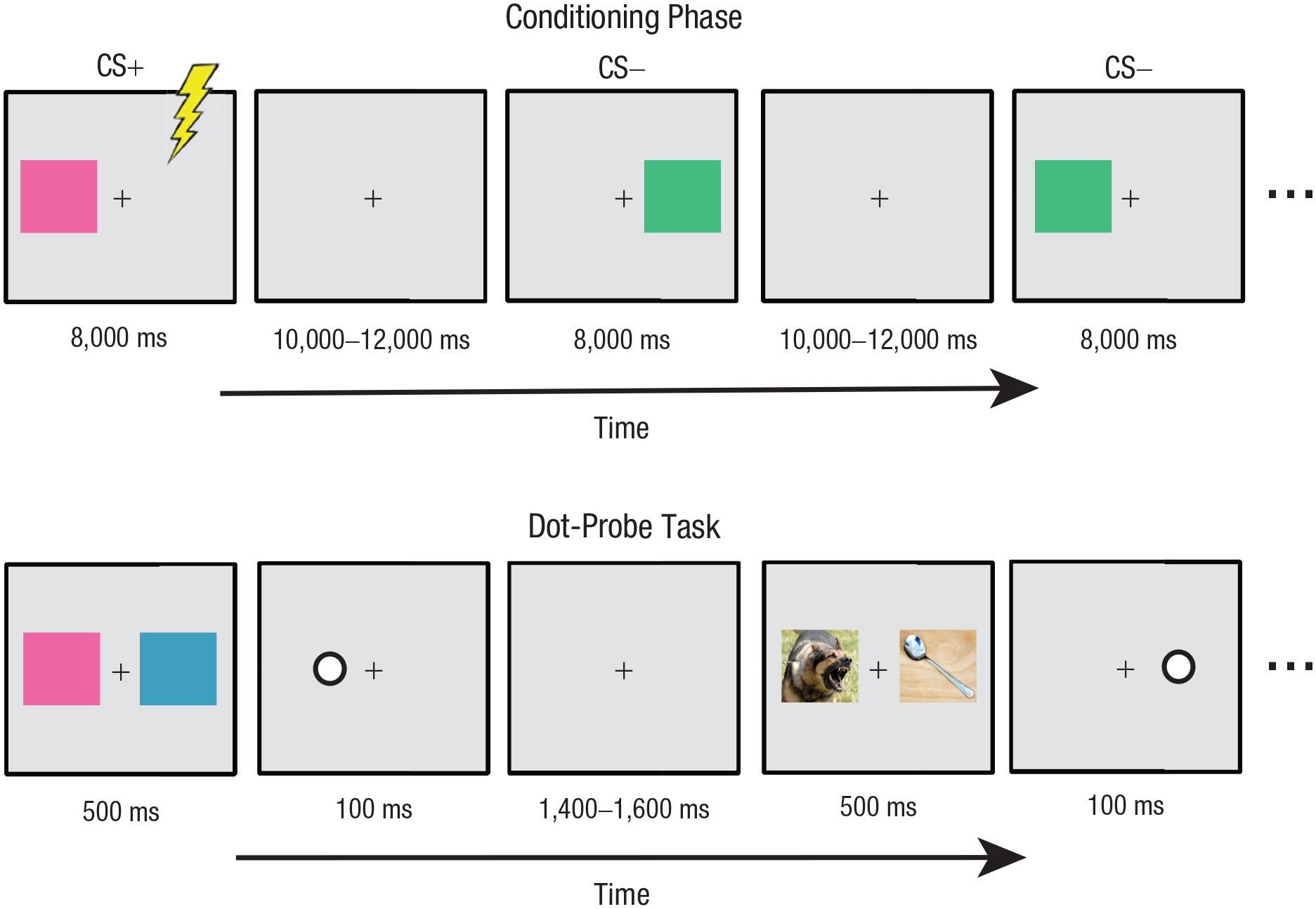
Example trials in the conditioning phase (top) and example trials in the dot-probe task (bottom). Note that stimuli are not to exact scale; see text for actual sizes used in the experiment.
Each stimulus subtended 7.3° × 5.7° of visual angle and was centered 4.4° to the left or right of a fixation cross subtending 0.4° × 0.4°. Following the offset of the stimulus, a fixation screen was presented for a jittered intertrial interval (ITI) of 10,000 ms to 12,000 ms (rectangular distribution).
Participants completed a total of 20 trials. The CS+ and CS– appeared with equal probability, evenly divided between left and right visual field presentations; all trial types were randomly intermixed. On eight of the 10 CS+ trials (80% reinforcement), an electric shock occurred during the last 500 ms of the CS+ presentation and coterminated with the CS+. The CS– was never paired with shock. Participants were instructed to count the number of shocks and to remember which color was associated with shock. Startle probes (50-ms white-noise bursts presented over speakers at 100 dB) were administered to verify that the conditioning manipulation was successful. Five startle probes were presented before the task began to habituate participants to the startle and establish a baseline; during conditioning, a startle probe was presented during each stimulus presentation (both CS+ and CS– trials) at a randomly selected time between 5,000 ms and 7,000 ms after stimulus onset; startle probes were administered on six randomly selected trials during the ITI at a randomly selected time between 5,000 ms from the start of the ITI and 1,000 ms before the next stimulus was presented. After conditioning, participants completed a questionnaire asking how many shocks were delivered as well as the perceived likelihood of being shocked for each of the two colors on a 5-point scale from 1 (certainly not shocked) to 5 (certainly shocked).
Dot-probe task
After conditioning, participants performed a dot-probe task. Example trial sequences are presented in Figure 1. On some trials, stimuli were selected from the set of four colored rectangles, including the CS+ and CS– from the conditioning task and the two colors the participant did not see in the conditioning task (termed untrained stimuli). On other trials, stimuli were selected from a set of 50 neutral and 50 threatening images chosen from the International Affective Picture System (IAPS; Lang, Bradley, & Cuthbert, 2008). Neutral photos included photos of buildings, household objects, and people with neutral facial expressions. Threatening photos included photos of animals attacking the viewer, assault and abduction scenes, and pictures of guns.
All stimuli were presented on a gray background with a continuously visible black fixation cross. On each trial, either a pair of photos or a pair of colored rectangles was presented for 500 ms, one stimulus on each side of fixation. Each image in a pair subtended 7.3° × 5.7° of visual angle and was centered 4.4° to the left or right of a fixation cross subtending 0.4° × 0.4°. Immediately following the offset of the images, a probe stimulus was presented for 100 ms. The probe consisted of a white dot outlined in black subtending 0.8° in diameter, centered in the location of one of the previously presented images. Participants made a keypress on a gamepad (Logitech, Newark, CA) with the index finger of the left or right hand to indicate the location of the probe stimulus. Following the offset of the probe, a fixation screen was presented for a jittered ITI of 1,400 ms to 1600 ms (rectangular distribution). Participants were told that the images were irrelevant to the task and were instructed to respond as quickly and as accurately as possible to the probes while maintaining eye fixation in the center of the screen.
Participants completed three blocks of 320 trials for a total of 960 trials. All trial types were randomly intermixed. Of primary interest are the “mixed-emotion” threat trials, which allowed us to isolate the N2pc and PD and calculate traditional RT-based bias measures. There were two mixed-emotion threat trial types: (a) the CS+ paired with one of the untrained colors (CS+/untrained) and (b) a threatening photo paired with a neutral photo (pictorial threat/neutral). Each of the threat trial types was presented for 80 trials within a block (for a total of 240 trials across the experiment). Threat stimuli were presented with equal probability to the left and right visual field in each condition, and each untrained color was presented an equal number of times across the CS+ trials. The location of the probe was fully counterbalanced for each trial type, presented at the location of each stimulus side and type an equal number of times within a block of trials. We also presented trials pairing the CS– with one of the untrained colors (CS–/untrained); participants completed 80 CS–/untrained trials per block (for a total of 240 trials), fully counterbalanced. Because these trials do not help answer the main question of interest in the present study (i.e., how attention operates in the presence of threat), the results of these trials will not be presented. Note that the CS+ and CS– were never paired together. The remaining trials were “same-emotion” trials, in which the same image was presented to both the left and right visual field; participants completed 20 trials of each of the following four same-emotion trial types per block for a total of 60 trials each across the experiment: (a) CS+/CS+ pairs, (b) CS–/CS– pairs, (c) threat photo/threat photo pairs, and (d) neutral photo/neutral photo pairs. Because the N2pc, PD, and traditional RT-bias measures of primary interest to the current study cannot be calculated on the same-emotion trials, the results of these trial types will not be presented.
To ensure that the CS+/shock association was maintained, the CS+ was accompanied by shock on eight randomly selected mixed-emotion CS+ trials within a block (for a total of 24 trials across the experiment, a 10% reinforcement rate). Participants were informed that the CS+ still had a chance of being accompanied by shock on some trials but that the shocks were irrelevant to the task. Trials with shocks were excluded from all analyses. Short self-paced rest breaks were provided every 40 trials, and longer rest breaks were provided every 320 trials.
Extinction
After the dot-probe task, an extinction phase was administered to remove the association between the CS+ and shock. The extinction procedure was too brief to provide enough trials for examining averaged ERP waveforms, so the extinction data were not analyzed.
Physiological recording and analysis
The continuous EEG was recorded using a BrainVision actiCHamp recording system and actiCAP active electrodes (Brain Products GmbH, Munich, Germany). The electrodes were mounted in an elastic cap using a subset of the International 10/20 System sites (FP1, F3, F7, C3, P3, P5, P7, P9, PO7, PO3, O1, Fz, Cz, Pz, POz, Oz, FP2, F4, F8, C4, P4, P6, P8, P10, PO4, PO8, and O2). A ground electrode was located at AFz. The horizontal electrooculogram (HEOG) was recorded from electrodes placed lateral to the external canthus of each eye. The vertical electrooculogram (VEOG) was recorded from an electrode placed below the right eye. The EEG and EOG signals were recorded in single-ended mode using a customized version of PyCorder recording software. Startle eyeblink EMG was recorded from two 4-mm bipolar passive electrodes placed over the orbicularis oculi muscle below the right eye, and a third electrode on the forehead served as an isolated ground; these electrodes were removed after conditioning. The EEG, EOG, and EMG signals were filtered online with a cascaded integrator-comb antialiasing filter with a corner frequency of 260 Hz and then digitized at 1000 Hz.
Signal processing and analysis was performed in MATLAB (The MathWorks, Natick, MA) using EEGLAB toolbox (Delorme & Makeig, 2004) and ERPLAB toolbox (Lopez-Calderon & Luck, 2014). For the EEG channels, the direct current (DC) offset was removed, and the EEG was high-pass filtered with a half-amplitude cutoff of 0.1 Hz (noncausal Butterworth impulse response function, 12 dB/oct roll-off). Break periods longer than 2 s were removed from the continuous EEG records. Independent component analysis (ICA) was performed for each participant to identify and remove components that were clearly associated with eyeblink activity, as assessed by visual inspection of the waveforms and the scalp distributions of the components (Jung et al., 2000). The ICA-corrected EEG data were then referenced to the average of P9 and P10 (located adjacent to the mastoids). Stimulus event codes were shifted forward 28 ms in time to adjust for the onset latency delay of the LCD monitor (which was measured with a photosensor). The data were segmented for each trial beginning 200 ms before the onset of the images and continuing for 800 ms. Baseline correction was performed using the 200 ms before the onset of the images. The data were low-pass filtered with a half-amplitude cutoff of 30 Hz (noncausal Butterworth impulse response function, 12 dB/oct roll-off). Noisy channels were interpolated using a spherical interpolation algorithm; no interpolation was performed on the channels used for referencing or measurement. Segments of data containing artifacts were removed through semiautomated ERPLAB algorithms, including large voltage excursions, eye movements larger than 0.1° of visual angle during the time range of the N2pc and PD (detected using the step function described by Luck, 2014), or trials containing eyeblinks or HEOG during the stimulus presentation window.
For the startle analysis, the signal from the startle EMG channel was segmented beginning 50 ms before the onset of the startle probe and continuing for 250 ms. Baseline correction was performed using the 50 ms before the onset of the startle probe. The EMG data were band-pass filtered with half-amplitude cutoffs at 28 Hz and 256 Hz (noncausal Butterworth impulse response function, 24 dB/oct roll-off), rectified, and smoothed using a 10-point running average. Artifact rejection was performed for the EMG signal in the −50-ms to 10-ms time window relative to startle probe onset to remove segments with eyeblinks or large voltage deflections in the baseline period. Startle eyeblink magnitude was measured as the largest local peak amplitude on individual trials using a time window of 20 ms to 200 ms. Peak amplitude values were averaged across trials, separately for startles presented during the CS+, CS–, and ITI.
RT was defined as the time of the button press relative to the onset of the probe on correct trials only; RTs were averaged separately for each condition. Trials with incorrect behavioral responses or RTs of < 200 ms or > 1,000 ms (relative to probe onset) were excluded from all analyses. Accuracy was calculated as the percentage of correct trials per condition within the acceptable RT range.
To examine the allocation of attention to threat and whether attention operated differently in the context of pictorial versus to conditioned threat, we isolated the N2pc and PD components time-locked to the onset of the image pairs at posterior electrode sites (P7 and P8, as in our previous studies; Kappenman et al., 2014, 2015) relative to the location of the threatening stimulus separately for the CS+ and pictorial threat trials. Specifically, we first created separate average waveforms for the hemisphere that was contralateral to the threatening stimulus (i.e., left hemisphere electrode sites for right-side threat and right hemisphere electrode sites for left-side threat) and the hemisphere that was ipsilateral to the threatening image (i.e., right hemisphere electrode sites for right-side threat and left hemisphere electrode sites for left-side threat). We then created contralateral-minus-ipsilateral difference waveforms for conditioned threat and for pictorial threat. The N2pc and PD were measured from the resulting difference waves in each participant.
Given the novelty of our experimental design, we did not have justifiable a priori predictions about the time course of the N2pc and PD in the present study, and previous studies have shown that the PD component can vary over a broad time window depending on the task and stimuli used. We could have chosen time windows for measuring the N2pc and PD on the basis of a visual inspection of the grand average ERP waveforms; however, this would bias us to obtain statistically significant results that might capitalize on noise in the waveforms (see Luck & Gaspelin, 2017). In addition, the time course of the N2pc and PD components could reasonably vary from participant to participant, which would make it difficult to identify a single time window to use for measurement of these components across all participants. Therefore, we used a procedure introduced and validated by Sawaki, Geng, and Luck (2012) in which the N2pc and PD are measured using broad time windows that do not require a priori predictions about the time course of the components. Because the N2pc and PD are opposite in polarity and their amplitudes would partially or wholly cancel each other out using traditional mean amplitude measures over a time window that included both components, we instead calculated negative area (area below the zero-voltage line) and positive area (area above the line) from each participant to quantify the N2pc and PD, respectively.
The amplitude of the N2pc was calculated as the mean negative area using a time window of 150 ms to 300 ms following the onset of the image pairs for each threat type. The amplitude of the PD was calculated as the mean positive area using a time window of 200 ms to 400 ms following the onset of the image pairs for each threat type. This made it possible to determine whether an N2pc (negative area) and/or a PD (positive area) were present in response to each type of threat. However, area measures are necessarily biased to be greater than zero because some negative activity and positive activity will typically be present in the waveform regardless of whether there is an N2pc or PD. To account for this, we used a nonparametric permutation approach that used permutations of the data to estimate the distribution of values that would be expected from noise alone (using the noise in the actual data) and determined whether the area measures were significantly larger than these values (instead of comparing the area measures with zero). This is becoming an increasingly popular approach in neuroscience (Groppe, Urbach, & Kutas, 2011; Maris, 2012; Maris & Oostenveld, 2007; Sawaki et al., 2012).
To accomplish this, we simulated no difference between the contralateral and ipsilateral voltages by randomly assigning trials for each participant to threat-left or threat-right conditions separately for pictorial threats and conditioned threats. For example, a trial on which the CS+ was presented on the left would be randomly assigned to a CS+ left or a CS+ right presentation, regardless of the actual location of the CS+ on that trial. If there is no real difference between the contralateral and ipsilateral voltages, then it should not matter which side is labeled as containing the threatening image. Consequently, we can estimate the negative and positive area that would occur by chance in the absence of a true difference by randomizing the assignment of trials to conditions, creating average noise waveforms, and measuring the negative and positive area from the noise waveforms.
To ensure that our estimates were accurate, we repeated this procedure 1,000 times to obtain a probability distribution, which reflects the likelihood of obtaining a given negative area during the N2pc time window and the likelihood of obtaining a given positive area during the PD time window if the null hypothesis is true (i.e., if there is no true difference between the contralateral and ipsilateral sites). We compared the observed negative area and positive area measured from the actual ERP waveforms with these randomly permuted values from the noise waveforms. The p value was then estimated by calculating the number of negative (or positive) permuted areas in the noise waveform calculations that were equal to or larger than the observed negative (or positive) area in the actual waveform and dividing by the total number of simulated permutations (in this case, 1,000).
Repeated measures analysis of variance (ANOVA) and t tests were used with a two-tailed α level of .05 for all statistical tests, and probability values were adjusted when appropriate with the Greenhouse-Geisser epsilon correction for nonsphericity (Jennings & Wood, 1976). Measures of effect size, including η2 values for ANOVAs and Cohen’s d with confidence intervals (CIs) for t tests, are provided for all tests. Pearson’s correlations were used to examine the relationship among measures. Split-half reliability analyses were conducted to examine the psychometric properties of each measure by computing correlations of the averages between odd-numbered trials and even-numbered trials, corrected using the Spearman-Brown formula (Anastasia & Urbina, 1997).
Given the limitations of traditional null hypothesis statistical testing, we also computed Bayes factors for each key statistical comparison using JASP software (Version 0.9.1), which implements the method of Rouder, Speckman, Sun, Morey, and Iverson (2009) for t tests and the method of Wetzels and Wagenmakers (2012) for correlations. The default scale factors were used (Cauchy scale = 0.707 for t tests and stretched β prior width = 1.0 for correlations). Bayes factors quantify the relative likelihood of obtaining the data given that the alternative hypothesis is true relative to the likelihood given that the null hypothesis is true. Following convention, we use BF10 to denote the relative strength of evidence for the alternative hypothesis and BF01 to reflect the relative strength of evidence for the null hypothesis (BF10 and BF01 are simply reciprocals).
Results
Conditioning
We first used the startle probe data to determine whether the conditioning phase was successful in associating the CS+ with the shock. Overall, the startle response varied across the CS+ (M = 67.86, SE = 7.27), CS– (M = 50.52, SE = 6.81), and ITI (M = 46.78, SE = 6.55) in a one-way ANOVA, F(2, 94) = 37.62, p < .001, η2 = .445. Follow-up pairwise t tests confirmed that startle magnitude was significantly larger during the CS+ than during the CS–, t(47) = 6.21, p < .001, d = 0.897, 95% confidence interval (CI) = [0.558, 1.229], and the ITI, t(47) = 7.46, p < .001, d = 1.077, 95% CI = [0.717, 1.430]; the magnitude of the startle response did not differ significantly during the CS– and ITI, t(47) = 1.78, p = .081, d = 0.257, 95% CI = [−0.032, 0.543].
The subjective likelihood of being shocked was also rated by participants as significantly higher for the CS+ (M = 4.33, SD = .476) than for the CS– (M = 1.06, SD = 0.320) stimulus, t(47) = 45.85, p < .001, d = 6.618, 95% CI = [5.253, 7.951].
Dot-probe task
Behavior
Table 1 provides mean accuracy (percentage correct) and mean RT for the mixed-emotion trials on threat-congruent trials (i.e., when the probe appeared at the location of the CS+ or pictorial threat stimulus) and on threat-incongruent trials (i.e., when the probe appeared at the location of the untrained color or the neutral photo). Mean accuracy was near ceiling on all trial types (> 98%) and will not be considered further.
Behavioral and Event-Related Potential (N2pc and PD) Measures
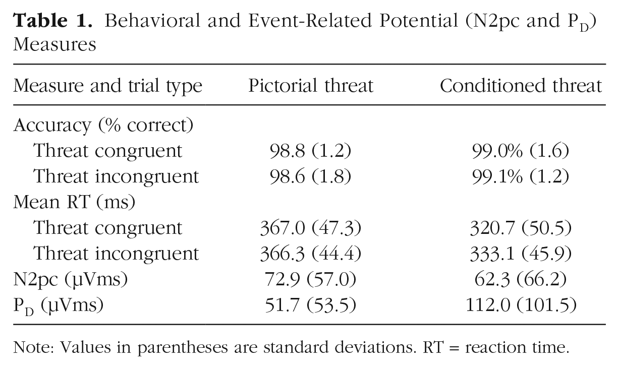
Note: Values in parentheses are standard deviations. RT = reaction time.
The mean RTs were analyzed in a 2 × 2 ANOVA with factors of threat type (conditioned threat vs. pictorial threat) and trial type (threat-congruent vs. threat-incongruent). For the conditioned threat stimuli, participants were faster on threat-congruent trials than on threat-incongruent trials (i.e., a bias for threat), but RTs were nearly identical on threat-congruent and threat-incongruent trials for the pictorial threat stimuli (i.e., no bias). RTs were also faster overall on conditioned threat trials than on pictorial threat trials. This led to a significant main effect of threat type, F(1, 47) = 448.41, p < .001, η2 = .905; a significant main effect of trial type, F(1, 47) = 6.33, p = .015, η2 = .119; and a significant Threat Type × Trial Type interaction, F(1, 47) = 10.52, p = .002, η2 = .183. Follow-up analyses confirmed that these results were driven entirely by faster RTs on threat-congruent compared with threat-incongruent trials on conditioned threat trials, t(47) = −3.03, p = .004, d = −0.437, 95% CI = [−0.732, −0.139], BF10 = 8.5). The Bayes factor indicated that the conditioned threat data were 8.5 times more likely to be obtained under the alternative hypothesis of a difference between threat-incongruent and threat-congruent trials than under the null hypothesis. Consistent with some previous studies, no significant RT difference was found between threat-incongruent and threat-congruent trials on pictorial threat trials, t(47) = 0.484, p = .630, d = 0.070, 95% CI = [−0.214, 0.353], BF01 = 5.7. The Bayes factor indicated that the pictorial-threat data were 5.7 times more likely to be obtained under the null hypothesis than under the alternative hypothesis. These analyses do not merely show the absence of evidence for the allocation of attention to the pictorial threat stimuli; the Bayes factor provides positive evidence for the absence of a difference in RT between threat-incongruent and threat-congruent trials for the pictorial threat stimuli. By contrast, the Bayes factor provided evidence for a bias to the CS+ stimulus on the conditioned threat trials.
We also examined the internal reliability of the traditional RT bias measure (threat-incongruent RT − threat-congruent RT) separately for conditioned threat and pictorial threat. The split-half reliability was near zero for pictorial threat trials (r = −.043, p = .772), replicating the low reliability we observed for this measure in our previous studies (Kappenman et al., 2014, 2015). By contrast, the split-half reliability was excellent for CS+ trials (r = .895, p < .001), indicating that conditioned threat stimuli in the present study elicited internally reliable RT bias effects.
Event-related potentials
Figure 2 (top) displays grand average contralateral-minus-ipsilateral ERP difference waveforms for each threat type time-locked to the onset of the image pairs and collapsed across the P7 and P8 electrode sites. Mean area measures for each component are shown in Table 1. An N2pc can be seen with a peak latency of approximately 200 ms on both pictorial threat and conditioned threat trials. The N2pc was followed by a prominent PD peaking around 350 ms on CS+ trials; however, little or no PD was present for pictorial threat stimuli.
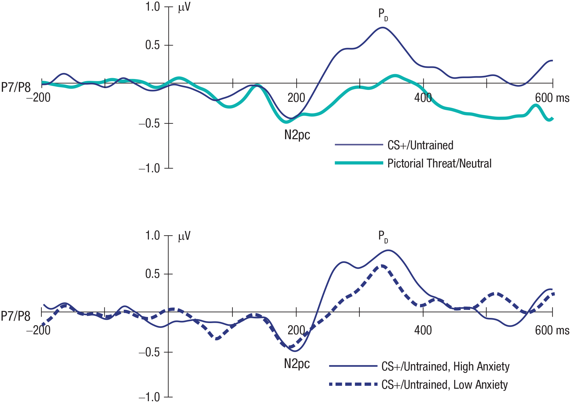
Grand average contralateral-minus-ipsilateral event-related potential (ERP) difference waveforms time-locked to the onset of the images collapsed across the P7 and P8 electrode sites overlaid for the pictorial threat (light blue line) and conditioned threat stimulus (CS+; dark blue line) trial types (top). Grand average contralateral-minus-ipsilateral ERP waveforms for the CS+/untrained trials as a function of a median split of high (dark blue line) compared with low (dashed blue line) trait anxiety (bottom). A digital low-pass filter was applied offline before plotting the waveforms (Butterworth impulse response function, half-amplitude cutoff = 20 Hz, 12 dB/oct roll-off).
To assess the statistical significance of these effects, we first performed permutation analyses to determine whether significant N2pc and PD components were present in response to each type of threat stimulus (i.e., whether the N2pc and PD components were significantly larger than would be expected on the basis of noise alone). A statistically significant N2pc was present in response to both pictorial threat (p < .001) and conditioned threat (p < .001) stimuli, reflecting a significant initial allocation of covert visual attention to both types of threat. In addition, the PD that followed the N2pc was statistically significant (p < .001) on conditioned threat trials, indicating that the initial allocation of attention to the CS+ was followed by a significant suppression of attention to the CS+. By contrast, the PD was not significantly greater than would be expected from the noise level on pictorial threat trials (p = .197). Unfortunately, no straightforward method exists for computing Bayes factors corresponding to these permutation analyses.
We next examined whether the amplitudes of the N2pc and PD components differed significantly on the basis of the type of threat stimulus presented. Because this involves comparing two trial types rather than comparing one trial type with chance, conventional analyses could be used instead of permutation analyses. The amplitude of the N2pc did not differ between pictorial threat and conditioned threat trials, F(1, 47) = 0.751, p = .391, η2 = .016, BF01 = 4.4, and the Bayes factor provided positive evidence that the initial allocation of attention to threat was consistent across threat types. By contrast, the PD was significantly larger in response to conditioned threat compared with pictorial threat, F(1, 47) = 16.74, p < .001, η2 = .263, BF10 = 145, indicating a greater suppression of attention to threat in response to conditioned threat compared with pictorial threat stimuli.
To assess the internal reliability of the ERP measures, we calculated the split-half reliability of the N2pc and PD separately for each threat type. N2pc area on odd-numbered compared with even-numbered trials was moderately reliable for both pictorial threat (r = .535, p < .001) and conditioned threat (r = .595, p < .001). This replicates our previous studies (Kappenman et al., 2014, 2015). On conditioned threat trials, PD area exhibited good reliability (r = .726, p < .001). For the pictorial threat trials, on which no significant PD was observed, the split-half reliability was lower but still significant (r = .378, p = .008), indicating that some stable individual differences in PD area were present even though the average PD was not different from the noise level.
Correlations
The mean score on the trait scale of the STAI was 38.33 (SD = 9.43, Mdn = 35.5, range = 21–55); these scores are in the expected range according to published norms for this age group (M = 36, SD = 10; Spielberger et al., 1983). To examine the relationship between anxiety and our measures of threat bias, we examined the correlation (Pearson’s r) between the trait anxiety scores and each RT and ERP measure separately for the pictorial threat and conditioned threat trial types. Scatter plots showing the relationship between anxiety and each bias measure are shown in Figure 3.
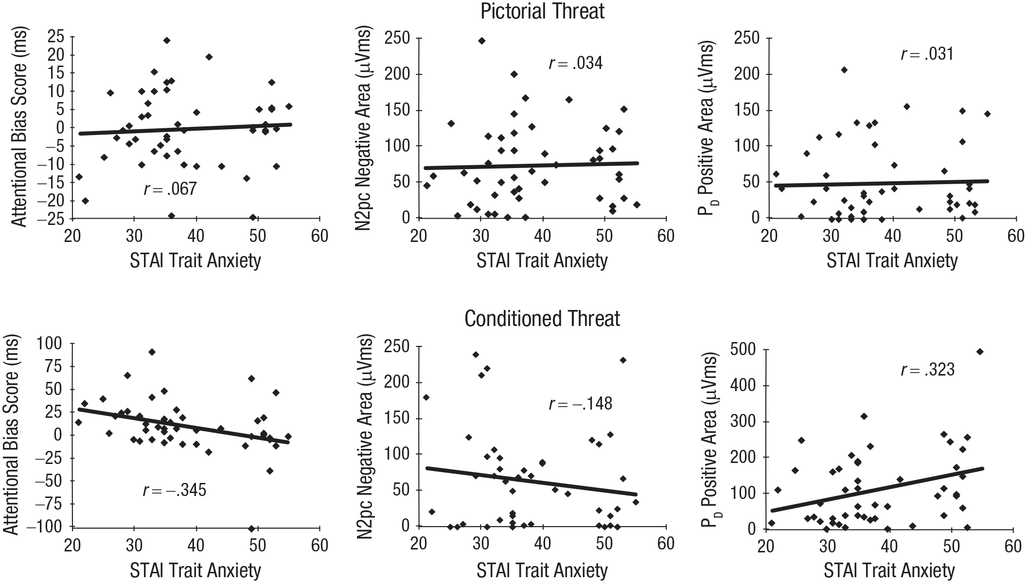
Scatterplots (with best-fitting regression lines) for the pictorial threat trials (top) and conditioned threat (CS+) trials (bottom) showing each threat bias measure as a function of State-Trait Anxiety Inventory scores for the response time measure of attentional bias (threat-incongruent minus threat-congruent; left), N2pc area amplitude (center), and PD area amplitude (right). Note that the y-axis scale varies across plots.
As in our previous study (Kappenman et al., 2014), there was no correlation between the RT measure of threat bias (threat-incongruent RT minus threat-congruent RT) and anxiety on pictorial threat trials (r = .067, p = .652, BF01 = 5.0) or between anxiety and N2pc area for pictorial threat (r = .034, p = .819, BF01 = 5.4). Likewise, anxiety and the PD on pictorial threat trials was uncorrelated (r = .031, p = .834, BF01 = 5.4). Note that the Bayes factors provide positive evidence for the lack of a correlation.
In contrast to pictorial threat, RT bias (calculated as RT on threat incongruent minus threat congruent trials) and anxiety (r = −.345, p = .016, BF10 = 2.9) were correlated on conditioned threat trials. This negative relationship between RT bias and anxiety is consistent with either decreased attention to threat or greater avoidance of threat in anxious individuals. Anxiety was uncorrelated with the amplitude of the N2pc on conditioned threat trials, results that were similar to pictorial threat trials (r = −.148, p = .315, BF01 = 3.4). However, there was a significant positive correlation between anxiety and the amplitude of the PD on conditioned threat trials (r = .323, p = .025, BF10 = 2.0), reflecting a larger PD (greater suppression of attention) to conditioned threat in participants with higher levels of anxiety. 1
The relationship between the amplitude of the PD and anxiety was confirmed in the ERP waveforms by calculating separate grand averages for participants with low versus high levels of anxiety (median split). As shown in Figure 2 (bottom), the PD was much larger in the high-anxiety subgroup than in the low-anxiety subgroup. We also examined whether the magnitude of the PD was correlated with RT bias. Although this correlation did not reach significance, there was a negative correlation between PD amplitude and RT bias (r = −.264, p = .070, BF10 = 0.884), reflecting a potential trend for greater suppression of attention to the CS+ location (i.e., a larger PD) to be associated with decreased attention to threat and/or greater avoidance of threat.
Discussion
In the present study, we identified novel relationships among attention, threat, and anxiety by using a new framework to isolate attentional processes associated with selection and suppression in the context of standard pictorial threat stimuli (i.e., photos of weapons, attacking animals, etc.) and conditioned threat stimuli (i.e., colored shapes aversively conditioned with electric shock). Although both types of threat elicited an initial selection of attention (an N2pc), we found no evidence that anxiety is related to increased selection of threat. This is contrary to the prediction of the widely held attentional bias hypothesis. Instead, anxiety was selectively related to reactive suppression of threat, reflected in a larger PD to conditioned threats for individuals with higher levels of anxiety. This is the first study to link differences in the magnitude of a neural signature of suppression of emotional stimuli with anxiety.
An association between anxiety and behavior was also obtained only in the context of conditioned threats, with RT-bias scores consistent with decreased attention to threat and/or increased avoidance of threat in anxious individuals. Moreover, ERP and behavioral measures of bias to conditioned threats were characterized by excellent psychometric properties. The relationship between the PD and RT bias did not reach significance in the present study, suggesting that attentional suppression alone cannot account for the entire pattern of behavioral results exhibited in the dot-probe task. This may be reflective of the fact that whereas the PD is a specific index of attentional suppression, RTs represent a combined measure of many distinct cognitive processes, which may also play an important role in anxious reactions to threats (Mogg & Bradley, 2018). Alternatively, given that there was a trend toward a relationship between PD and RT bias, the present study may simply have been underpowered to detect such a relationship. This is an important issue to be explored in future studies.
Note that we found associations between attention and anxiety for conditioned threat stimuli but not for the traditionally used pictorial threat stimuli. We suspect this is because the conditioned threats, which are associated with a real threat (i.e., electric shock), are stronger and more consistent elicitors of a threat response than photographs of weapons, attacking animals, and the like. Each participant likely has individual responses to the threats depicted in the photos based on personal experiences, and therefore, there may be significant variability across trials and across participants in reactions to these photos. Consistent with this possibility, measures of RT bias to the photos were completely unreliable, whereas measures of RT bias to the conditioned threats had high reliability. It is possible that photos that specifically match a given individual’s threat bias may reveal associations between attention and anxiety that are not observed with unselected, general threat photos. For example, one study provided some initial evidence that pictures of angry faces may elicit increased selection among socially anxious individuals (Reutter et al., 2017). However, no evidence of a behavioral bias to angry faces was found in socially anxious individuals in this study, in contrast to the behavioral bias we observed with conditioned threats (Reutter et al., 2017). Moreover, although this previous study did not explicitly examine the PD, no evidence of active suppression of the angry faces is visible in their figures. Thus, even in cases in which photographic stimuli are targeted to a given individual, they still may not be sufficiently threatening to reveal the full pattern of bias in anxiety demonstrated with conditioned threats in the present study.
The present results pose a significant challenge to the general hypothesis that heightened attentional bias toward threat aids in the establishment or maintenance of elevated anxiety levels. Within this general framework, researchers have proposed that anxious individuals pay increased attention to threat (MacLeod & Clarke, 2015; Mathews & MacLeod, 2002), have difficulty disengaging from threat (Fox, Russo, Bowles, & Dutton, 2001; Fox, Russo, & Dutton, 2002; Yiend & Mathews, 2001), or have a generalized deficit in attentional control (Derakshan & Eysenck, 2009; Eysenck et al., 2007). We found no evidence for these attentional deficits in anxiety in the present study, consistent with other dot-probe studies (see e.g., Kappenman et al., 2014, 2015; Kruijt et al., 2019). Instead, the present study showed that both conditioned and pictorial threat stimuli elicited an initial allocation of attention irrespective of an individual’s anxiety level. We further found that all individuals could rapidly engage inhibitory mechanisms to suppress attention to the location of the conditioned threat stimulus. Indeed, anxious individuals showed more suppression than nonanxious individuals.
Although more research is needed to understand the causes and consequences of this enhanced suppression effect, we provide a speculation: If individuals with greater levels of anxiety experience a more aversive response when attention is captured by a threat stimulus, this may lead to a more intense reactive suppression of the stimulus (i.e., avoidance). This may in turn draw cognitive resources away from other stimuli or tasks such that the cognitive deficits observed in anxiety may be a consequence of efforts to suppress or avoid threat-related stimuli rather than occurring because resources are engaged in the enhancement of threat. Moreover, suppression of attention to threat may be negatively reinforcing and more so for anxious individuals. In this way, the current results fit well with decades of research linking anxiety to avoidance behaviors (Rescorla & Solomon, 1967).
These results may also have important implications for ABM treatment, which typically trains anxious individuals to shift attention away from threatening stimuli (for a recent review, see Mogg & Bradley, 2018). Specifically, the present results implicate an entirely new mechanism of reactive suppression as an important treatment target for attention-related training in anxiety—at least in the context of conditioned threat. It will be important for future research to extend the present work to individuals with clinical levels of anxiety and to examine the efficacy of treatment aimed at reducing avoidance in mitigating anxiety.
Footnotes
Acknowledgements
We thank Daniel Kapulkin for help with task programming and Amanda Ng for help with data collection.
Transparency
Action Editor: Erin B. Tone
Editor: Kenneth J. Sher
Author Contributions
E. S. Kappenman and G. Hajcak developed the study concept and designed the study. Data collection was performed by R. Geddert. Data analysis was completed by E. S. Kappenman, J. L. Farrens, and R. Geddert. E. S. Kappenman, J. J. McDonald, and G. Hajcak wrote the manuscript, and R. Geddert and J. L. Farrens provided feedback. All of the authors approved the final manuscript for submission.