Wagner’s Hypothesis: An Empirical Verification

Abstract

This study explores the relationship between public expenditure (PE) and gross domestic product (GDP) to verify whether the Wagner’s hypothesis holds good in the Indian context. We cover the period from 1970 to 2013 and use econometric tools like Autoregressive Distributed Lag Model (ARDL) test to check the long-run and causal relationship among the variables. The results of the bounds test suggest that there exists cointegration between PE and GDP, but we found weak evidence for Wagner’s hypothesis as well.

Keywords

Wagner’s hypothesis bounds test cointegration error correction public expenditure and GDP.

Introduction

Public expenditure (PE) plays a significant role in an economy, not only to ensure economic stability but also to generate employment opportunities and accelerate economic growth and development. It also plays a vital role in alleviating mass poverty and reducing the severity of income inequality and some other elementary problems, as mentioned below:

To build up economic overheads, for example, roads, railways, irrigation, power, etc., or undertake social overheads such as hospitals, schools, etc. Both of these help to boost growth and development of the economy.

To get balanced regional growth by channelizing economic resources in a proper way and, as a result, help in sorting out the problem of regional imbalances of the economy.

To develop mineral resources such as agriculture and industry.

The role of PE is more important in case of developing countries as compared to developed countries, the objective being distribution of economic resources to achieve a social optimum. Since the 19th century, several attempts have been made to analyze the nature, significance and scope of PE. Later on, these attempts developed into different theories of public expenditure in the literature of public finance. Some of the important theories are Adolf Wagner’s hypothesis, Wiseman–Peacock hypothesis, Musgrave and Rostow’s development model and Clark’s Critical Limit hypothesis. The present study focuses only on Adolf Wagner’s hypothesis.

Wagner’s Hypothesis: A Theoretical Aspect

According to Wagner, ‘There are inherent tendencies for the activities of the different layers of the government (such as central and state government) to increase both extensively and intensively’ (Bhatia, 2011). More clearly there is a functional relationship between the growth of an economy and the growth of the government activities (Bhatia, 2011).

Wagner was one of those scholars who realized the positive correlation between the level of economic deve-lopment and the size of the public sector. Though he was not the first person to state this relation, he was the first one who attempted to show an empirical demonstration (Chang, Liu, & Caudill, 2004). Wagner’s concept is based on the experience of early stages of industrialization, particularly in Germany and also in the rest of Europe, which suggested that growth of PE was a natural consequence of economic growth. His view subsequently became a law, known as ‘Wagner’s Law’. Wagner identified three main factors behind the increase in government spending. These are as follows:

Over a period of time, as long as an economy matures (i.e., along with growing population, industrialization and urbanization economy will move from low economic development, especially in traditional societies with limited production that barely attain the minimum level of potential output, to high mass consumption of the contemporary period, wherein consumers concentrate on durable goods and hardly remember the subsistence concerns of previous stages), there will be need for government to play an important role in administrative and protective capacity apart from enhancing social welfare.

As long as the economy expands, government expenditure also expands on various social welfare activities like health, education, infrastructure, recreation facilities, etc.

Advancement in science and technology of a country results in higher government expenditure on various new projects. Due to increased expenditure, it would be demanded of the government to provide several economic services for which private sector will remain indeterminate (Khan, 1990).

Apart from these, where merit goods and natural resources monopolies are concerned, government will manage on purpose the production process in order to ensure fair and justifiable distribution of the natural resources.

It is not clear from the various explanations provided by different scholars whether Wagner was trying to suggest an increase in:

Absolute level of public expenditure.

The ratio of government spending to gross national product (GNP).

The proportion of public sector in the total economy (Bhatia, 2011).

This ambiguity in his theory has provided a broad base for further research. Consequently, different studies adopted different versions of Wagner’s hypothesis. However, the number of versions has often remained limited to six. All the six versions tested in the literature are given in Table 1.

The present study seeks to confirm the existence of long-run relationship between PE and GDP in all these six versions of the hypothesis in Indian context. It is divided into five sections. While Section 1 gives an introductory note, Section 2 reviews existing literature on Wagner’s hypothesis, Section 3 brings out sources of database and methodology, Section 4 demonstrates empirical work, and finally, Section 5 sums up the article with concluding remarks.

Table 1.

Six Versions of Wagner’s Hypothesis

S. No.	Functional Form	Version
		Absolute Version
1.	$L n (R G E) = β_{1} + β_{2} L n (R G D P) + u_{t}$	Peacock and Wiseman (1961)
2.	$L n (\frac{R G E}{P}) = β_{1} + β_{2} L n (\frac{R G D P}{P}) + u_{t}$	Gupta (1967)
3.	$L n (R G E) = β_{1} + β_{2} L n (\frac{R G D P}{p}) + u_{t}$	Goffman (1968)
4.	$L n (R G C E) = β_{1} + β_{2} L n (R G D P) + u_{t}$	Pryor (1969)
		Relative Version
5.	$L n (\frac{N G E}{N G D P}) = β_{1} + β_{2} L n (\frac{R G D P}{P}) + u_{t}$	Musgrave (1969)
6.	$L n (\frac{N G E}{N G D P}) = β_{1} + β_{2} L n (R G D P) + u_{t}$	Mann (1980)

Sources: Demirbas (1999); Verma and Arora (2010).

Notes: RGE: Real Government Expenditure; RGDP: Real Gross Domestic Product; P: Population; RGCE: Real Government Consumption Expenditure; NGE: Nominal Government Expenditure; NGDP: Nominal Gross Domestic Product.

Literature Review

In the history of public finance, several studies have been conducted over a period of time to test Wagner’s hypothesis, and the evidence for its holding out has been mixed. A brief review of recent studies is presented here.

Studies Based on Developed and Developing Countries

Ram (1987) examined Wagner’s hypothesis by using an individual country time series data and inter-country cross section data for 115 countries for the period 1950–1980, using annual data. He found that sign and strength of covariance between income and government’s expenditure vary considerably across different countries of the world. The hypothesis is supported by 69 countries and refuted in the remaining 46 countries. On the other hand, the results from the cross-section data did not support the hypothesis.

Mohsin, Sridevi and Kamaiah (1995), using annual data for the period 1961–90 in their study, found results supporting Wagner’s hypothesis in a group of 20 developing countries.

Cotsomitis, Harnhirun and Kwan (1996) used annual data to test the long-run validity of Wagner’s hypothesis in the case of China. The study used Engle–Granger and cointegration tests and the results were in support of Wagner’s hypothesis.

Chletsos and Kollias (1997) examined the causal relationship between government expenditure and GDP in Greece for the period 1958–1993. They used cointegration and error correction mechanism for their study after decomposing the government consumer spending into civilian and military. Their study found that growth of GDP did not show any effect on civilian expenditure. On the other hand, military expenditure seemed to have been influenced by economic growth.

Abizadeh and Gray (1985) examined the relationship between economic development and public expenditure growth in South Korea. Their study concluded that the government’s spending had positively and significantly affected the private sector’s income.

Asseery, Law and Perdikis (1999) examined Wagner’s hypothesis in Iraq by using the disaggregated data on the variables both in nominal and real terms for the period 1950–1980. Their study revealed weak evidence for the existence of Wagner’s hypothesis when income and several other forms of expenditure are represented in nominal terms. However, once expenditure is taken in real terms, they found a reverse direction of causality, that is, the variables take Keynes’ hypothesis rather than Wagner’s. Chow, Cotsomitis and Kwan (2002) conducted their study in UK for the period 1948–1997. By using bivariate cointegration, multivariate Granger causality test, Zivot–Andrews test for stationarity, etc., they found evidence in favour of Wagner’s hypothesis.

Dilrukshini (2009) analyzed the relationship between PE and economic growth in Sri Lanka for the period 1952–2002. By using cointegration test for a long-run relationship, he concluded that there exists no empirical support either for Wagner’s hypothesis or for Keynes’ hypothesis.

Afzal and Abbas (2010) investigated the applicability of Wagner’s hypothesis in Pakistan for the period 1960–2007. Using disaggregate data, they found that the hypothesis held only between 1981 and 1991 for the period under consideration.

Pahlavani, Abed and Pourshabi (2011) investigated the applicability of Keynes’ and Wagner’s hypotheses in case of Iran for the years from 1960 to 2008. They concluded that unidirectional causality runs from economic growth to the size of government.

Kumar, Webber and Fargher (2012) examined Wagner’s hypothesis in case of New Zealand over the period from 1960 to 2007. By applying bounds test, Engle–Granger cointegration test, Phillips and Hansen’s fully modified ordinary least squares and Johansen’s time series tests, they found results in favour of Wagner’s hypothesis.

Dada and Adewale (2013) examined Wagner’s hypothesis for Nigeria during the period 1961–2011. By using Johansen multivariate cointegration test and vector error correction mechanism, they found evidence for long-run causality running from real GDP to government’s spending. However, no such relationship was found for a short run. Therefore, the study concluded that Wagner’s hypothesis is not a short-run but a long-run phenomenon.

Oktayer and Oktayer (2013) analyzed the relationship between government expenditure and economic growth in Turkey by using annual time series data for the period 1950–2010. By using trivariate causality test and autoregressive distributed lag (ARDL) model, they concluded that there is no long-run relationship between government’s expenditure and national income.

Studies on India

Singh and Sahni (1984) examined the causality between national income and total public expenditure as well as for various components of public expenditure for the period between 1950 and 1981 in case of India. The study revealed a feedback relation among variables. Furthermore, it confirmed both Wagner’s hypothesis (income causes public expenditure) and Keynes’ hypothesis (public expenditure causes national income).

Mohsin, Bhat and Kamaiah (1992) examined the causal relationship between public expenditure and national income in case of India with the help of cointegration and Error Correction Modelling for the period from 1950–51 to 1988–89. By applying the standard Granger-causality test, they found a unidirectional causal relationship from public expenditure to income in both real and nominal terms which supports the Keynes’ hypothesis. Khundrakpam (2003) examined the public sector spending and economic growth in India between years 1960–61 and 1996–97. By using the ARDL model, the study found a stable long-run relationship between public sector spending and national income in India. As the causality was running from public sector spending to national income, the study confirmed the applicability of Keynes’ hypothesis for the given period.

Verma and Arora (2010) analyzed the relationship between government spending and economic growth in India for the period between 1950 and 2008 and found Wagner’s hypothesis both in pre- and post-reform period.

Ranjan and Chintu (2013) analyzed the applicability of Wagner’s hypothesis in Indian economy by using annual time series data for the years between 1970–71 and 2010–11. The results showed that economic growth is cointegrated with the size of government. Further, the Granger causality test, conducted by Ranjan and Chintu (2013), confirmed that a unidirectional causality flows from economic growth to the size of government, confirming the applicability of Wagner’s hypothesis in Indian context.

The review of literature reveals that studies based on Wagner’s hypothesis have produced mixed evidences. The present study attempts to verify Wagner’s hypothesis by using ARDL cointegration approach on the six different versions of the hypothesis.

Database and Research Methodology

Availability of a good database is a necessary condition for any empirical analysis. One should keep in mind, ‘It is capital mistake to theorize before one has data. Insensibly one begins twist facts to suit theories, instead of theories to fit facts’ (as quoted by Sir Arthur Conan Doyle through his famous character Sherlock Holmes). Lack of reliable data on a broad set of variables is a major problem in developing countries. The dataset used in the present study for the years from 1970 to 2013 has been taken from a secondary source, that is, the RBI Handbook of Statistics on Indian Economy. This dataset contains annual observations for variables like real and nominal GDP, population, total expenditure on consumption made by government, etc.

Stationarity Test

To verify long-run relationship between government expenditure and total output, we used time series data. Before proceeding with any time series analysis, it is necessary to test for the stationarity of the processes.

To check whether a given time series process is stationary or non-stationary, several stationarity tests are available, namely, Graphical Method, Correlogram test and the Unit Root test. The stationarity of the process may be assessed by two unit root tests, namely, Augmented Dickey–Fuller (ADF) test and Phillips–Perron (PP) test. Although the bounds test for cointegration does not require that all variables should be integrated of order one {I (1)}, it is important to conduct the stationarity test in order to ensure that no variable is integrated of order two {I (2)}. If the variables of order {I (2)} are integrated,, the F-test will be spurious or the computed F-statistic produced by Pesaran, Shin and Smith (2001) and Narayan (2005), will not be valid (Pahlavani, Abed, & Pourshabi, 2011; Odhiambo, 2009).

Cointegration Test: ARDL Approach

Our study aimed to empirically examine Wagner’s hypothesis in case of India. According to Wagner’s hypothesis, there is co-movement between PE and GDP in the long run. To test this hypothesis empirically we used cointegration analysis. ‘Cointegration, an econometric property of time series variable, is a precondition for the existence of a long-run or equilibrium economic relationship between two or more variables’ (Ray & Ray, 2012). Pesaran et al. (2001) have developed the ARDL or ARDL bounds testing approach for cointegration. It has some advantages over conventional cointegration testing approaches (Engle & Granger, 1987; Johansen, 1988; Johansen & Juselius, 1990, among others). First, the bounds test is easy in procedure as compared to other methods of cointegration; it allows the cointegration relationship to be estimated by Ordinary Lest Square (OLS) once the lag order of the model is identified. Second, it can be used when the series are integrated of order zero or one, or even if it is a combination of two. Third, ARDL model involves just a single equation set-up, making it simple to implement and interpret. Finally, both short-run and long-run estimators can be simultaneously estimated.

The ARDL bounds test approach used in this study may be specified as follows:

\begin{matrix} Δ L P E_{t} = C_{0} + β_{1} L P E_{t - 1} + β_{2} L G D P_{t - 1} + \\ \sum_{i = 1}^{p} α_{i} Δ L P E_{t - i} + \\ γ ​_{j} Δ L G D P_{t - j} + ε_{t} \end{matrix}

(1)

where, β₁ and β₂ are the long-run multiplier, C₀ is the drift and ε_t is the white noise error term, Δ is the first difference operator and, LGDP and LPE are the log of GDP and the log of public expenditure, respectively.

The first step in the ARDL bounds testing approach is to estimate Equation (1) by OLS method to test for the existence of a long-run relationship among variables. On the basis of F-statistic, the null hypothesis of no cointegration against the presence of cointegration (alternative hypothesis) among the variables is tested.

Two critical values are given by Pesaran et al. (2001) for the cointegration test, the lower critical bound and the upper critical bound. The lower critical bound assumes that variables are integrated of order zero {I (0)} and upper critical bound assumes that variables are integrated of order one {I (1)}. When the F-statistic exceeds the upper critical bound, the null hypothesis of no cointegration will be rejected, that is, it would show that there is cointegration. If the F-statistic is below the lower critical bound then the null hypothesis of no cointegration will be accepted, which would mean there is no cointegration among variables. If F-statistic falls in between lower and upper bounds, the result will be inconclusive.

If there exists a long-run relationship among variables, the second step is to estimate the long-run model for LPE.

L P E_{t} = C_{0} + \sum_{i = 1}^{p} δ_{1} L P E_{t - i} + \sum_{j = 1}^{p} δ_{2} L G D P_{t - J} + ε_{t}

(2)

By using different information criteria, we select the order of the variables in the ARDL model. There are various criteria for lag selection such as Akaike Information Criteria (AIC), Schwarz Bayesian Information Criterion (SBIC), Factor Price Equalization (FPE), Likelihood Ratio (LR) and Hannan–Quinn Information Criterion (HQC), etc.

In the third and final step of the bounds testing procedure, we obtain the short-run dynamic parameters by estimating an error correction model associated with the long-run estimates. This is specified as follows:

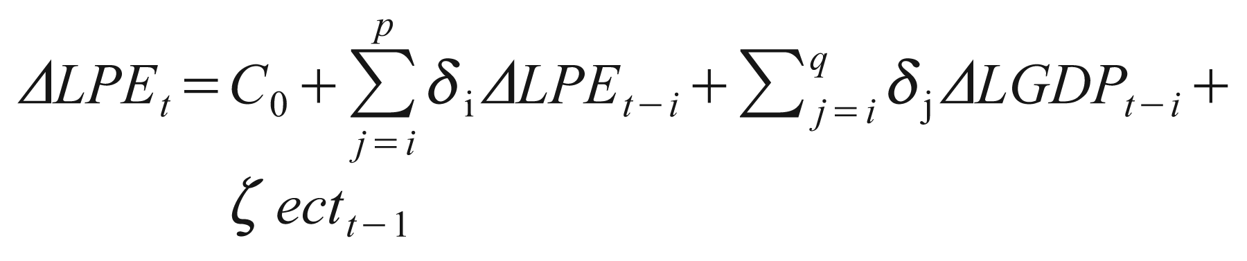
\begin{matrix} Δ L P E_{t} = C_{0} + \sum_{j = i}^{p} δ_{i} Δ L P E_{t - i} + \sum_{j = i}^{q} δ ​_{j} Δ L G D P_{t - i} + \\ ζ e c t_{t - 1} \end{matrix}

(3)

In Equation (3), δ_i and δ_j are the short-run dynamic coefficients of the model’s convergence to equilibrium and ζ is the speed of adjustment. Here, in order to estimate the speed of adjustment of the dependent variable to independent variable(s), the lagged level variables in Equation (1) are replaced by ect_t_– 1 where ‘ect’ is the error correction term derived from the long-run relationship. If the value of speed of adjustment is zero, it means that there exists no long-run relationship. If it is between −1 and 0, there exists partial adjustment; a value smaller than −1 indicates that the model over-adjusts in the current period; a positive value implies that the system moves away from equilibrium in the long run (Oktayer & Oktayer, 2013).

Finally, some of the diagnostic and stability tests are used to evaluate our model. The diagnostic tests check for serial correlation, autoregressive conditional heteroscedasticity (ARCH), the functional form of the model and normality of residual term. In addition, the stability tests of long-run and short-run parameters are conducted by using the cumulative sum of recursive residuals (CUSUM) and the cumulative sum of squares (CUSUM square) of recursive residuals.

Empirical Analysis

Unit Root Test Results

The result of ADF test failed to reject the null hypothesis of unit root at the initial stage, that is, variables are non-stationary at levels. But at first difference, null hypothesis gets rejected, that is, variables become stationary at first difference. To complement the ADF results, we also performed PP test that is more robust to measure autocorrelation and heteroscedasticity. PP test also supports the previous test results. The result of the ADF and PP unit root test are reported in the Table 2.

Table 2.

Unit Root Test Results

Variables	ADF		PP
	Level	First Difference	Level	First Difference
LRGDP	−1.985	−7.483*	−2.004	−7.881*
	(0.5929)	(0.00)	(0.583)	(0.00)
LRPGDP	−1.6208	−7.4632*	−1.630	−7.847*
	(0.7681)	(0.00)	(0.764)	(0.00)
LRGEXP	−2.889	−6.346*	−2.855	−6.419*
	(0.1759)	(0.00)	(0.187)	(0.00)
LRGCEXP	−2.989	−5.954*	−2.955	−5.958*
	(0.1759)	(0.00)	(0.156)	(0.00)
LRPGEXP	−2.698	−6.3289*	−2.600	−6.394*
	(0.2425)	(0.00)	(0.282)	(0.00)
LNGEXP/NGDP	−2.85	−3.912*	−2.403	−6.540*
	(0.1889)	(0.02)	(0.373)	(0.00)

Source: Calculated by authors.

Note: * indicates statistically significant at 1% level of significance. The values in parenthesis are probability values.

Results of Cointegration Test

In the next step, we performed ARDL bounds test to examine the existence of cointegration. The bounds test approach on all six alternative versions of Wagner’s hypothesis has been used to examine long-run relationship between the variables. To know the appropriate lag length of the variables in ARDL model, we used the AIC and SBIC criteria. Order of the variables in different versions is presented in Table 3.

Table 3.

Lag Selection Criteria

Models	Lags	AIC	SBC
A: Peacock and Wiseman	1	−7.36	−7.10
B: Gupta	1	−7.31	−7.06
C: Goffman	1	−7.28	−7.02
D: Pryor	1	−7.50	−7.24
E: Musgrave	1	−10.83	−10.57
F: Mann	1	−10.87	−10.62

Source: Calculated by authors.

At lag order one, there is a strong evidence of cointegration between PE and GDP for all the versions of Wagner’s hypothesis because the calculated F-statistic is greater than the critical values of upper bound (given in Pesaran et al., 2001) at 5 per cent level of significance. The results are reported in Table 4.

Table 4.

Bounds F-test for Cointegration

Models	Dependent Variable	F-test Statistic	Cointegration
Model A	LRGXP	2.334	NO
	LRGDP	33.090	YES
Model B	LPRGEXP	2.403	NO
	LPRGDP	21.900	YES
Model C	LRGEXP	2.030	NO
	LPRGDP	17.000	YES
Model D	LRGCEXP	1.360	NO
	LRGDP	12.330	YES
Model E	L(NGEXP/NGDP)	1.880	NO
	LPRGDP	25.540	YES
Model F	L(NGEXP/NGDP)	1.810	NO
	LRGDP	58.330	YES

Source: Calculated by authors.

Coefficient diagnostic and residual diagnostic (against serial correlation Lagrange Multiplier [LM] test, histogram–normality test and ARCH LM test for heteroscedasticity) results are shown in the Table 5 for each of the models. Further, stability of the parameter over the sample period (1970–2013) has been tested using the CUSUM and CUSUM square tests. The respective test results for all the versions or models are reported in Figures 1–6.

Figure 1.

Source: Calculated by authors.

Figure 2.

Source: Calculated by authors.

Figure 3.

Source: Calculated by authors.

Figure 4.

Source: Calculated by authors.

Figure 5.

Source: Calculated by authors.

Figure 6.

Source: Calculated by authors.

Table 5.

Diagnostic Tests

	Diagnostic Tests
Model	Normality Test	LM Test	ARCH Test	RESET Test
A: Peacock and Wiseman	1.078(0.58)	0.577428(0.4523)	0.345837(0.5599)	0.205935(0.6527)
B: Gupta	1.08(0.58)	0.431(0.516)	0.165(0.687)	0.621(0.436)
C: Goffman	0.93(0.63)	0.507(0.48)	0.578(0.452)	0.012(0.914)
D: Pryor	2.36(0.31)	0.395(0.533)	1.148(0.29)	0.352(0.557)
E: Musgrave	15.19(0.00)	0.811(0.373)	0.028(0.867)	1.405(0.243)
F: Mann	13.26(0.00)	1.163(0.373)	0.019(0.887)	1.4(0.244)

Source: Calculated by authors.

Note: The values in parenthesis are probability values.

Based on the performance of different diagnostic tests, the results reported in different tables depict that all models are fit to be used for the estimation purpose. They also show that there is an absence of autocorrelation, functional form misspecification, heteroscedasticity in the models, and the errors follow the normal distribution.

Coefficient Stability Tests

The parameter stability or coefficient stability of any model has been considered to be crucial. The coefficient stability is tested by plots of CUSUM and CUSUM squares given in Figures 1–6. In all the graphs the straight lines represent critical bounds at 5 per cent significance level, since the plot of these two tests do not cross the critical value line except in Musgrave and Mann versions, indicating a stable long-run relationship between government expenditure and GDP. Overall, we can conclude that coefficients are stable in the long run.

Long-run Relationship

Long-run estimated coefficients for all the versions have been reported in Table 6. The result shows that only in Peacock and Wiseman model, the government expenditure coefficient is significant at 5 per cent, whereas in Goffman model, the long-run coefficient of government expenditure is significant at 10 per cent. In the models of Gupta, Pryor, Mann as well as Musgrave, the long-run coefficients are insignificant. Since only in the case of Peacock and Wiseman version the long-run coefficients are significant, it may be concluded that there is only small evidence of cointegration between PE and GDP.

Table 6.

Long-run Coefficients

	Long-run Coefficients
Model	Dependent Variable	Regressors	Coefficient	Probability
A: Peacock and Wiseman	LRGDP	LRGEC	1.549**−0.926	0.0230.789
B: Gupta	LRPGDP	LRGEXPC	2.4211.634*	0.3010.004
C: Goffman	LRPGDP	LRGXPC	1.304***−6.419	0.0820.187
D: Pryor	LRGDP	LRGCEC	1.580.01	0.230.999
E: Musgrave	LRPGDP	L(NGEXP/NGDP)C	−0.6660.73	0.5530.72
F: Mann	LRGDP	L(NGEXP/NGDP)C	−0.9485.153	0.63640.176

Source: Calculated by authors.

Note: *, **, *** indicate level of significance at 1%, 5% and 10% level of significance, respectively.

Error Correction Model (ECM)

In the next phase of analysis, the focus was on ECM, in which we gather the direction of causality between the variables by testing the significance of coefficient of the lagged error correction term (ζ) (Odhiambo, 2010). Further, we also go for the short-run dynamics of the variables in ECM. Accordingly, the short-run versions of ARDL models are estimated and the respective results are reported in the Tables 7 and 8.

Table 7.

Short-run Dynamics

Short-run Coefficients
Model	Variable	Coefficient	Prob.
A: Peacock and Wiseman	D(LRGE)D(LRGE(−1))ecm(−1)	0.195−0.119*−0.031	0.0010.0260.374
B: Gupta	D(LRPGEXP)D(LRPGEXP(−1))ecm(−1)	0.201−0.123*−0.023	0.0010.0250.527
C: Goffman	D(LRGXP)D(LRGXP(−1))ecm(−1)	0.192−0.114*−0.033	0.0010.0310.353
D: Pryor	D(LRGDP(−1))D(LRGCE)ecm(−1)	−0.2290.176**−0.024	0.1420.010.546
E: Musgrave	D(L(NGEXP/NGDP))ecm(−1)	0.0230.035*	0.5570.00
F: Mann	D(L(NGEXP/NGDP))ecm(−1)	0.0180.019*	0.6360.003

Source: Calculated by authors.

Note: *, **, *** indicate level of significance at 1%, 5% and 10% level of significance, respectively.

Table 8.

Wald Test Results

Wald Test Based on ECM
Model	F-statistics	Chi-square
A: Peacock and Wiseman	460.12(0.00)	920.24(0.00)
B: Gupta	450.892(0.00)	901.783(0.00)
C: Goffman	407.934(0.00)	815.868(0.00)
D: Pryor	297.684(0.00)	595.369(0.00)
E: Musgrave	5823.405(0.00)	11646.81(0.00)
F: Mann	14143.99(0.00)	28287.97(0.00)

Source: Calculated by authors.

Note: The values in parenthesis are probability values.

An ECM model has two important parts: estimated short-run coefficients and error correction term (ECT). ECT provides the feedback or speed of adjustment from short-run to long-run equilibrium. There are two important things about ECT. The ECT coefficient should be significant on the one hand and on the other hand it must be negative, so that it provides further proof of stable long-run relationship (Banerjee, Dolado, & Mestre, 1998; Shahbaz & Rahman, 2010).

The test results of the short-run model show that ECT is very weak in all versions except those of Musgrave and Mann. In case of Musgrave and Mann, ECT is significant but the coefficient is positive. Also, in case of other versions, ECT is negative as well as insignificant. Hence, we cannot rely on ECM for short-run causality.

Summary and Concluding Remarks

The relationship between PE and GDP has remained a debatable issue in the public finance literature. It gave rise to various schools of thought, which tried in their own way to limit or expand the economic boundary of the government. While some supported the involvement of government in the core economic activities, others restricted its role to the mere provision of peace and security. Both Keynes’ and Wagner’s hypotheses deal with PE and GDP. If causality runs from PE to GDP, then it shows that the relationship supports Keynes’ hypothesis. On the other hand, if causality runs from GDP to PE, then the relationship supports Wagner’s hypothesis. Hence, in case of Keynes, PE becomes the cause (i.e., the independent variable) and GDP becomes the effect (i.e., the dependent variable). In the case of Wagner, PE becomes the effect (i.e., the dependent variable) and GDP is the cause (i.e., the independent variable). In this sense, because of the cause and effect relation, the two hypotheses came to the forefront. One showed the importance of government expenditure to affect economic activity at different points of business cycle (Keynes’ hypothesis) and the other explained the historical expansion of government sector with respect to the spreading out of economic activities (Wagner’s hypothesis). A major difference between these two approaches is one of the directions of causality. In case of Wagner’s hypothesis, causality runs from GDP to PE while in Keynes’ hypothesis causality runs from PE to GDP. In the light of this background, the present study attempted to verify the applicability of Wagner’s hypothesis in Indian context empirically, by considering the time series data for the period 1970–2013.

Wagner’s hypothesis states that there exists a positive relationship between state activities and public expenditure. Because of some ambiguity in its functional form, different versions of the hypothesis have come up in the existing literature. These include, broadly, Goffman model, Gupta model, Mann model, Musgrave model, Peacock and Wiseman model and Pryor model.

To verify the long-run relationship between PE and GDP in case of India, we adopted ARDL cointegration approach. Due care was taken with respect to the functional form, serial correlation, normality assumption, heteroscedasticity and coefficient stability of the model. The results of the study showed that there exists a long-run relationship between PE and GDP and at the same time weak evidence was found in support of the Wagner’s hypothesis.

That support for the Keynes’ hypothesis was found is in line with the planning strategy that was followed in the country from the beginning of the 1950s. Since we had inherited a ruined economy at the time of independence, it was very difficult for private enterprises to come forward to manage a destabilized and weak economy. The intervention of government in the economic sphere was found to be the best solution to overcome all the hindrances and build a strong economic base for the years to come. Accordingly, the government got involved on a large scale in creating economic opportunities for the growing population. One can easily follow the story by looking at the steady increase in public spending over the years. In fact, the growth of public sector has served its purpose to a great extent to give a big push to all economic activities, although the setting off of problems like inefficient use of resources cannot be neglected. It was only after the reforms of the 1990s that we notice some decrease in the proportion of public spending, but it does not diminish the importance of involvement of government in various economic activities.

In a nutshell, throughout the world once again a wave has started supporting the importance of the public sector to manage and correct the market failures that have damaged the economic prosperity of billions of people both in developed and developing countries. India is not the only country to involve the government sector in indispensable economic activities side by side with the private sector, as it did over a period of time after planning. Thus, our findings from this study do not contradict the Keynes’ hypothesis where government sector influences the economic growth of the country. Government spending has boosted national output to a great extent throughout the period under investigation.

References

Abizadeh

, & Gray

(1985). Wagner’s law: A pooled time series, cross section comparison. National Tax Journal, 38(2), 209–218.

Afzal

Md.

, & Abbas

(2010). Wagner’s law in Pakistan: Another look. Journal of Economics and International Finance, 2(1), 12–19.

Asseery

A. A.

, Law

, & Perdikis

(1999). Wagner’s law and public expenditure in Iraq: A test using disaggregated data. Applied Economics Letters, 6(1), 39–44.

Banerjee

, Dolado

, & Mestre

(1998). Error-correction mechanism tests for cointegration in a single-equation framework. Journal of Time Series Analysis, 19(3), 267–283.

Bhatia

H. L.

(2011). Public finance (26th Edition). New Delhi: Vikas Publishing.

Chang

, Liu

, & Caudill

S. B.

(2004). A re-examination of Wagner’s law for ten countries based on cointegration and error-correction modelling techniques. Applied Financial Economics, 14(8), 577–589.

Chletsos

, & Kollias

(1997). Testing Wagner’s law using disaggregated public expenditure data in the case of Greece: 1958–93. Applied Economics, 29(3), 371–377.

Chow

Y. F.

, Cotsomitis

J. A.

, & Kwan

A. C.

(2002). Multivariate cointegration and causality tests of Wagner’s hypothesis: Evidence from the UK. Applied Economics, 34(13), 1671–1677.

Cotsomitis

J. A.

, Harnhirun

, & Kwan

A. C.

(1996). Co-integration analysis and the long-run validity of Wagner’s hypothesis: Evidence from the People’s Republic of China. Journal of Economic Development, 21(2), 1–10.

10.

Dada

M. A.

, & Adewale

O. A.

(2013). Is Wagner’s law a myth or a reality? Empirical evidence from Nigeria. International Journal of Development and Economic Sustainability, 1(1), 123–137.

11.

Demirbas

(1999). Cointegration analysis—causality testing and Wagner’s law: The case of Turkey, 1950–1990 (Volume 93). Volume 99 of Discussion papers in economics. Leicester, UK: University of Leicester, Department of Economics.

12.

Dilrukshini

W. A.

(2009). Public expenditure and economic growth in Sri Lanka: Cointegration analysis and causality testing. Central Bank of Sri Lanka, Staff Studies, 34(1–2), 51–68.

13.

Engle

R. F.

, & Granger

C. W.

(1987). Co-integration and error correction: Representation, estimation, and testing. Econometrica: Journal of the Econometric Society, 55(2), 251–276.

14.

Johansen

(1988). Statistical analysis of cointegration vectors. Journal of Economic Dynamics and Control, 12(2), 231–254.

15.

Johansen

, & Juselius

(1990). Maximum likelihood estimation and inference on cointegration—with applications to the demand for money. Oxford Bulletin of Economics and Statistics, 52(2), 169–210.

16.

Khan

A. H.

(1990). Wagner’s law and the developing economy: A time series evidence from Pakistan. Indian Economic Journal, 38(1), 115–123.

17.

Khundrakpam

J. K.

(2003). Public sector spending and economic growth in India. RBI Occasional Papers, 22(1, 2, & 3), 1–17.

18.

Kumar

, Webber

D. J.

, & Fargher

(2012). Wagner’s law revisited: Cointegration and causality tests for New Zealand. Applied Economics, 44(5), 607–616.

19.

Mohsin

Md.

, Bhat

K. S.

, & Kamaiah

(1992). Causality between public expenditure and national income in India. Asian Economic Review, 34(2), 375–390.

20.

Mohsin

Md.

, Sridevi

, & Kamaiah

(1995). Wagner’s law in developing countries: Evidence from time series analysis, Artha Vijnana, No. 3, 231–250.

21.

Narayan

P. K.

(2005). The saving and investment nexus for China: Evidence from cointegration tests. Applied Economics, 37(17), 1979–1990.

22.

Odhiambo

(2009). Energy consumption and economic growth nexus in Tanzania: An ARDL bounds testing approach. Energy Policy, 37(2), 617–622.

23.

Odhiambo

(2010). Energy consumption, prices and economic growth in three SSA countries: A comparative study. Energy Policy, 38(5), 2463–2469.

24.

Oktayer

, & Oktayer

(2013). Testing Wagner’s law for Turkey: Evidence from a trivariate cuasality analysis. Prague Economic Papers, No. 2, 284–301.

25.

Pahlavani

, Abed

, & Pourshabi

(2011). Investigating the Keynesian hypothesis and Wagner’s law on the size of government and economic growth in Iran. International Journal of Business and Social Science, 2(13), 170–175.

26.

Pesaran

M. H.

, Shin

, & Smith

R. J.

(2001). Bounds testing approaches to the analysis of level relationships. Journal of Applied Econometrics, 16(3), 289–326.

27.

Ram

(1987). Wagner’s hypothesis in time series and cross section perspective: Evidence from ‘real’ data for 115 countries. Review of Economics and Statistics, 69(2), 194–204.

28.

Ranjan

, & Chintu

A. K.

(2013). An application of Wagner’s law in the Indian economy: 1970–71 to 2010–11. Knowledge Horizons— Economics, 5(4), 138–144.

29.

Ray

, & Ray

I. A.

(2012). On the relationship between government’s developmental expenditure and economic growth in India: A cointegration analysis. Advances in Applied Economics and Finance, 1(2), 86–94.

30.

Shahbaz

, & Rahman

M. M.

(2010). Foreign capital inflows–growth nexus and role of domestic financial sector: An ARDL co-integration approach for Pakistan. Journal of Economic Research, 15(3), 207–231.

31.

Singh

, & Sahni

B. S.

(1984). Causality between public expenditure and national income. The Review of Economics and Statistics, 66(4), 630–643.

32.

Verma

, & Arora

(2010). Does the Indian economy support Wagner’s law? An econometric analysis. Eurasian Journal of Business and Economics, 3(5), 77–91.