



Abstract
The markets for agricultural crops have always been segmented. Although agricultural price policy in India is largely focused on declaring minimum support price (MSP), for select crops at all Indian levels the price for any crop has hardly been unique for the country. In this context, the paper tries to understand how far prices of paddy have been different across states. To what extent such price policies, primarily the public procurement system, are instrumental in the determination of actual price differentials realized by farmers across states. The paper draws its analysis from unit-level data of the 77th round of the National Sample Survey on the situation assessment of farmers (2018–2019). The paper evaluates some of the possible factors such as government procurements of paddy, land ownership patterns, percentage of farmers selling in the regulated markets, among others, in the context of price determination of paddy. The paper also seeks the link between local market price and average price in the regulated markets in different states.
Keywords
Introduction
Since the beginning of neoliberal reforms in India, the terms of trade for agriculture have remained largely unfavorable. Relative deterioration in the price of foodgrains along with increased volatility induced by exposure to the international market has been one of the major characteristics of post-reform agriculture in India. Falling share of public investment in agriculture along with the sharp reduction in input subsidies have put the entire sector under severe distress (De Roy, 2017). Some argued that the lack of reforms in the agricultural sector, particularly in terms of distortions in competitive market prices by public procurement price policy, has been responsible for such distress. Such policies are forcing farmers to cultivate particular foodgrains that government procurement is available for, and farmers are therefore unable to diversify production towards high-value crops largely based on market demand and supply (The Indian Express, 2022). It is further argued that instead of price support by the government, increased access to diversified markets, better research and development, and advancement of extension services would connect farmers with higher international value chains and thus be instrumental in increasing farmers’ income (The Indian Express, 2021).
However, such arguments are problematic in many respects. Firstly, international experiences reveal that the outcomes of rise of Global Agricultural Value Systems (GAVS) have been largely associated with the monopolistic concentration and control of resources, informalization and marginalization of labor, accentuated land alienation, deterioration of biodiversity, and increasing stress on livelihoods, with weakening of food security in large parts of the Global South (Jha & Yeros, 2019). Besides, relying more on global value systems and promoting exports has largely been counterproductive for developing countries primarily on two accounts; firstly, the international prices of primary commodities have been more volatile than the domestic prices; and secondly, existence of competitive demand and supply at the international level has been highly suspect on account of iniquitous global political influence on the markets (Kumar, 2019).
In this context, this study attempts to evaluate critically the agricultural price policies in India, particularly with respect to public procurement systems in providing better average price to farmers for rice. Since agriculture is an issue for states in India, and production conditions (Dev & Rao, 2010) and public procurement (Mohan & Kumar, 2018) vary largely across states, this study explores various dynamics associated with the difference in average price received by farmers across major states in India. The focus is also on identifying the set of correlates, particularly related to government procurement, responsible for such differential in prices. Furthermore, an attempt is made to explore the relationship between government procurement and local market (non-regulated market) prices across states. In other words, the paper explores the extent to which regulated market prices influence non-regulated market prices (local market prices) for paddy, as realized by farmers across states. Also, some other factors, such as land distribution, production and yields of crops, are also explored in the context of price realization of farmers across states.
Agricultural price policy in India is largely attributed to the establishment of minimum support prices (MSP) for various crops. The primary objective of MSP is to identify and fix a set of prices for the agricultural produce by ensuring basic viability of the agricultural operation (GoI, 2006). Fixation of MSP by the Government is primarily based on the changing cost of cultivation of the concerned crops. The cost of cultivation is generally calculated by the Commission for Agricultural Cost and Price. 1 However, only government agencies and government-regulated markets such as Agricultural Produce Marketing Committee (APMC) ensure MSP (at least) to farmers selling in those markets officially. No private selling agency is legally bound to give MSP to farmers for their produce (Singh & Bhogal, 2021). Also, with agriculture as a state affair in India and farming conditions varying substantially across states, the prices of crops are expected to be different across states despite the announcement of MSP at the pan-India level. Besides, since a part of agricultural produce is consumed locally and is perishable in nature, the transportation of crops from one region to another happens to be insufficient to reduce price gaps across states substantially.
In this study, the selection of paddy is based on the fact that the overwhelming proportion of farmers are engaged in the cultivation of paddy and the cultivation is spread over almost all the major states in the country. The analysis is based on the survey conducted during 2018–2019 as reported in the 77th round of the National Sample Survey Organization (NSSO) database. The price, in this study, is the rate of paddy received by the individual farmer which is calculated from the unit-level data. In the entire paper, gross farms are taken as the unit of analysis. 2 Seventeen major paddy-producing states have been included, namely Andhra Pradesh (AP), Assam (ASSM), Bihar (BIH), Chhattisgarh (CHHAT), Gujarat (GUJ), Haryana (HAR), Jharkhand (JHAR), Karnataka (KAR), Kerala (KER), Maharashtra (MAH), Madhya Pradesh (MP), Odisha (ODISH), Punjab (PUN), Telangana (TEL), Tamil Nadu (TN), Uttar Pradesh (UP), and West Bengal (WB).
The article is organized into four sections. The first section deals with procurement agencies and their role in overall procurement from farmers; the second incorporates patterns of price differentials across states; the third deals with Principal Component Analysis (PCM) for identifying a set of relevant factors affecting the price variation across states; and the fourth seeks to understand various correlates of price difference across states. Concluding remarks are provided at the end.
Procurement Agencies and Farmers’ Selling Patterns Across States
Broadly, the NSSO records procurement agencies such as local markets, input dealers, private food processing units, and contract farming agencies, as part of the non-price regulated agencies. Within these non- regulated agencies, the local market constitutes a significant proportion of total sale by farmers. On the other hand, procurement agencies, such as cooperatives, the APMC, government agencies, and Farmers Producer Organizations (FPOs), are largely considered as price-regulated procurement agencies in which MSP is applicable. As the system of MSP is not legally binding for private players, in all other agencies the price offered to the farmers is broadly market-determined (Narayanmurthi, 2021).
Table 1 shows the percentage of farmers selling their produce to various procurement agencies across states. The distribution is far from homogenous, and in some states like Kerala, Chhattisgarh, and Telangana, large number of farmers sell their produce in regulated markets like APMC, cooperatives, or to government agencies. While for some states, such as Haryana and Punjab, the ratio of farmers selling in the regulated market is reasonably high, for all other states, the proportion of farmers selling in the non-regulated markets is quite high and, within that, the ratio for local market is overwhelming. In fact, in Jharkhand, the proportion of farmers selling in the non-regulated market is as high as more than 99% (nearly 98% for local market alone). For some other states like Bihar, Assam, Karnataka, Uttar Pradesh, and West Bengal, this ratio was observed to be extremely high. As far as contract farming is concerned, Punjab observed that around 12% of paddy farmers sell their produce under contract, while in all other states the presence of contract farming is dismal. In Gujarat and Maharashtra, the number of farmers reported to be selling directly to the private food processor units is relatively higher than that of the other states. Thus, as is evident from Table 1, farmers in most of the states are relying more on non-regulated markets, particularly on local markets, for selling their produce, while for a few states like Kerala, Chhattisgarh, Telangana, Haryana, and Punjab, regulated markets have a relatively higher presence.
Distribution of Procurement by Agencies Across States.

One of the important factors affecting farmers selling in the regulated market is the availability of government procurement. In terms of absolute quantity, procurement has been highly skewed across states. Six states, namely Punjab (25.53%), Telangana (11.69%), Andhra Pradesh (10.82%), Odisha (10.02%), Chhattisgarh (8.94%), and Haryana (8.88%), constitute nearly 76% of total paddy procurement in the country (Table 2). However, their contribution in the production of paddy in the country remains less than 40%. More precisely, some states such as Punjab (88.39%), Haryana (87.29%), Kerala (80.45%), Telangana (77.81%), Chhattisgarh (60.84%), Andhra Pradesh (58.36%), and Odisha (57.5 %), the percentage of total government procurement out of total production of paddy was very high, while for states such as Gujarat (0.47%), Assam (1.95%), Karnataka (1.72%), Jharkhand (5.25%), Bihar (15.42%), and Maharashtra (17.7%), the ratio of procurement to production was very low.
Government Procurement and Price Related Indicators Across Select States.

Such heterogeneity in terms of availability of public procurement across states has been largely the function of the political economy of the state concerned. The public procurement of foodgrains in Punjab and Haryana remained historically much higher since the Green Revolution (GR) period. In fact, with the spread of GR in North Indian states, farmers both in Punjab and in Haryana gradually started to organize themselves into a strong lobby with a clear collective voice. Since then, in both states, the political presence of farmers’ lobbies remained evident, irrespective of the incumbent political party. Thus, the dominance of Punjab and Haryana in the overall public procurement of the country was obvious.
Among states with high levels of procurement, Chhattisgarh has been gaining significance. With a strong public distribution system (PDS), Chhattisgarh witnessed high demand for foodgrains for distribution. Such requirement could not be fulfilled by the quota of public procurement allocated by the center alone. Consequently, most of the public procurement in the state has been happening through the state procurement agencies (Banerjee, 2011). This has led to a sharp rise in the public procurement of rice over the years in Chhattisgarh. In case of Andhra Pradesh, though there was a decline in the share of procurement-production ratio during 1980s and 1990s, the ratio rose significantly since the early 2000s. The political collaboration between the first National Democratic Front government at the center and the Chandrababu Naidu-led government in Andhra Pradesh, particularly during the first half of 2000s (Raghavan, 2004), had a direct bearing on this shift, but after reaching a particular level, the procurement production ratio remained nearly stagnant in the state. 3 In fact, with the millers’ lobby in Andhra Pradesh being substantially instrumental in influencing in the procurement policy of the state, there has been a visible dominance of rice procurement instead of paddy. Besides, delay in payment through the official channel and poor procurement infrastructure are largely indicative of the lack of willingness of the state towards the farmers’ cause in the state (Murthy, 2011). Therefore, despite rising productivity and improvement in overall production in the state, there has hardly been any commensurate rise in the public procurement of paddy during the recent period. Nevertheless, the overall share in total procurement remained higher in Andhra Pradesh as compared to many of its neighboring states.
The case of Telangana is, however, different. After being separated from Andhra Pradesh, the state enacted the Food Security Act in 2015 and consequently increased its public procurement significantly since 2016. Therefore, Telangana followed a different trajectory than Andhra Pradesh in terms of enhanced PDS backed by increased public procurement. A similar pattern was observed in Kerala, which has been witnessing a strong PDS with relatively higher public procurement of rice for a longer period. In fact, with fast implementation of the Food Security Act, along with major reforms in the distribution systems (Thomas, 2017), Kerala’s public procurement also witnessed a rise in recent years. Odisha, with continuous improvement in the overall procurement infrastructure, has shown a rather steady growth in the procurement. Furthermore, the increasing inclusivity of farmers with a better price delivery system as compared to the other eastern states over the years (Kumar et al., 2022) has been remarkably effective in improving the procurement-production ratio over recent years.
Even though West Bengal has been one of the biggest producers of rice for long, the procurement under the central pool through the Food Corporation of India (FCI) remained extremely limited. In fact, when West Bengal initiated a local procurement scheme it was argued that the acquisition cost offered by the center has remained unfavorable to the state (Raghavan, 2004). Nevertheless, West Bengal, unlike Chhattisgarh, could not strengthen its PDS substantially during the most recent period and therefore the scope of higher local procurement systems with better local distribution was hardly realized in the state. Therefore, in spite of being a state with one of the highest rice productions in the country and home to probably the largest number of paddy-producing farmers, the non-regulated local market has been the primary recourse for the farmers in West Bengal.
The case of Bihar is interesting, where APMC was abolished in 2006. Even the restoration of Primary Agricultural Credit Societies (PACS) in Bihar could not improve the status of procurement in the regulated markets in any substantive manner (Kumar et al., 2022). Some limitations of PACS in this regard have been its omission error, local politics, and the state’s inadequate funding to carry out large procurement (Kumar, 2021). Furthermore, in the absence of any major political presence of a farmers’ union or farmers’ pressure group, the state’s reluctance towards increasing procurement remained largely visible. Besides, the conditions of the PDS in Bihar has largely remained precarious (Dreze et al., 2013) with extremely high leakage from PDS (Dreze & Khera, 2015). Although with the introduction of food coupons, there was some improvement in controlling the leakage (Choithani & Pritchard, 2015), the overall conditions of PDS remained far from satisfactory, despite the enactment of the National Food Security Act (NFSA). Thus, the abolition of APMC and the lack of proper functioning of PACS, along with a weak PDS systems culminated into low level of procurement of paddy in the state.
In all, the lack of political will, adverse center-state relations, the weak collective political voice of farmers, and insufficient demand for rice by the state due to poor PDS remained some of the important factors instrumental in lower procurement of rice in all other states. Sure enough, government procurement in states has been highly skewed in terms of both absolute quantity of procurement and the share of production across states. This has obvious bearing on the percentage of farmers selling in the regulated markets, as both cooperatives and direct government procurement have played crucial role in the entire regulated markets.
The states with higher percentage of government procurement to production show higher percentages of farmers selling in the regulated markets. Although this relationship seems trivial, in reality it is more complex. There are two possibilities due to which such a direct/straight relationship might not be fully explanatory. First, if in any states the proportion of large farmers is higher and they are the ones selling primarily into the regulated market, high procurement-to-production ratio does not necessarily denote higher percentage of farmers selling in the regulated market. Secondly, the numbers might not be conclusive if in some states middlemen are actively involved in purchasing paddy from the farmers at a relatively lower price than MSP, and then sell the procured paddy into the regulated markets. The percentage of total sale of paddy in quantity out of total reported government procurement (Table 2) shows that in case of Jharkhand (4.61%), Assam (9.48%), and Andhra Pradesh (10.37%), the total quantity sold in the regulated markets 4 as reported by farmers 5 constitute smaller portions of total procurement. This means that large proportions of government procurements are happening from non-farmers or middlemen in these states.
However, for some states like Karnataka, Gujarat, Chhattisgarh, and Telangana, this ratio is well above 100%, 6 which to a large extent confirms that most of the government procurement in those states is happening from the farmers directly. Here, the case of Karnataka and Gujarat is not much of importance because government procurement in the state has been meagre and only small proportions of farmers are selling in the regulated market. However, for Chhattisgarh and Telangana, higher procurement-production ratios and higher percentage of farmers selling in the regulated markets certainly imply that government procurement is overwhel- mingly happening from farmers directly. In all other states, there have been moderate gaps between government procurement and the farmers’ reported quantity of selling in the regulated markets, which confirms that government procurement is happening from both farmers and middlemen in those states. To what extent such gaps affects prices across states will be evaluated in latter part of this article.
Understanding the Structure of Price Differentials Across States
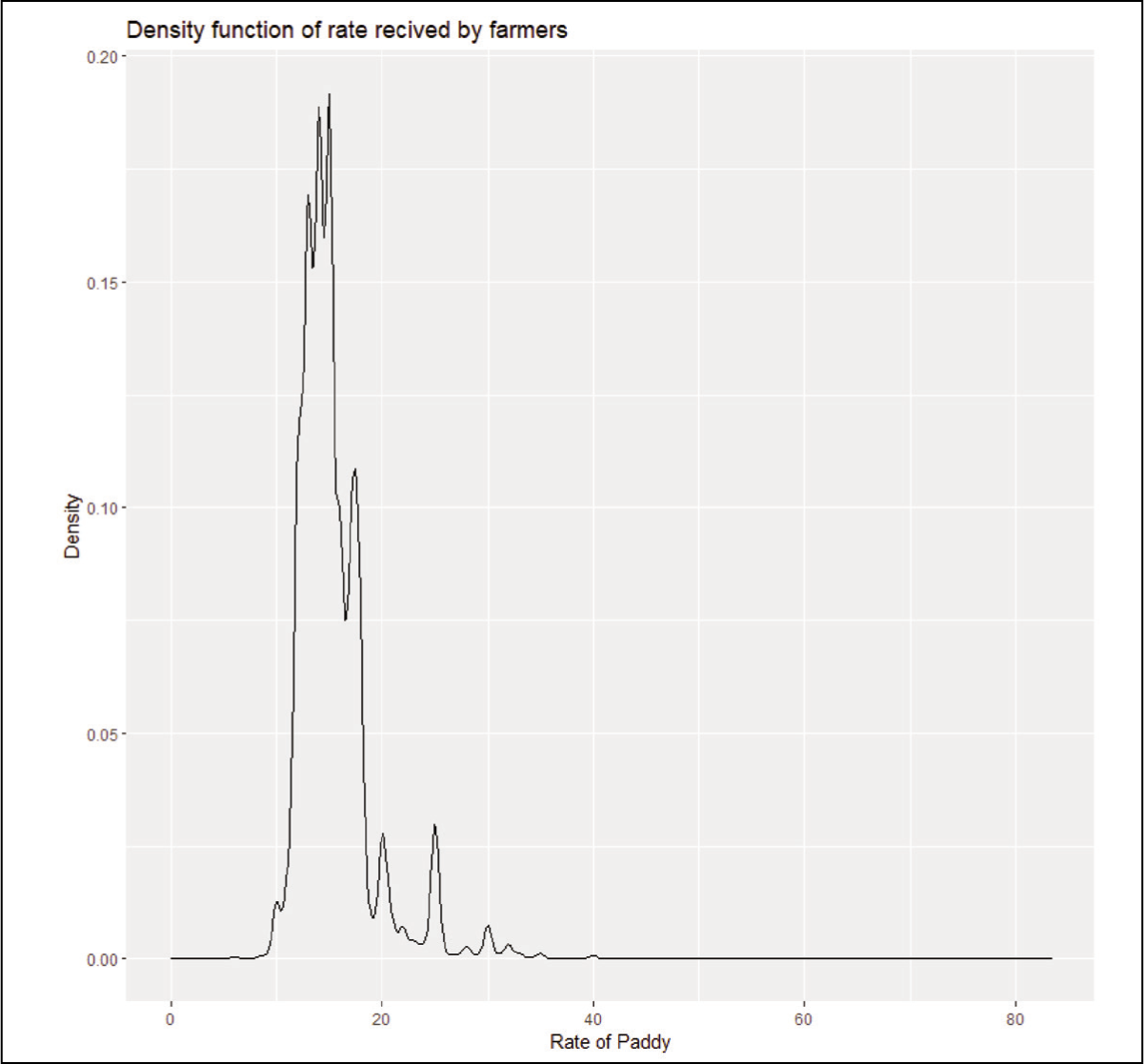
Before going into the details of state-specific price, it is important to understand the structure of prices at the national level. Figure 1 shows that the country is far from having a unique price, although the agricultural price policies are based on a single procurement price at the pan-India level. 7 Figure 1 confirms the presence of at least eight peaks (for price of paddy) ranging from as low as 15 to as high as 30 rupees per kilogram. Since agricultural markets are segmented across states and procurements are also a function of state policies, one can suspect that such variation could have some overlapping with the states. Analysis of the average price of paddy across states through the ANOVA test (Table 3) confirms that for all states average prices of paddy are not the same. The F value is completely significant.
The ANOVA Results for Testing Unique Price for All States.

Table 4 shows that average prices of paddy are different for the majority of the states in pairs. There are few pairs of states, such as Punjab and Chhattisgarh, Jharkhand and Odisha, Gujarat and Maharashtra, Andhra Pradesh and Gujarat, Karnataka and Madhya Pradesh, Karnataka and Andhra Pradesh, Tamil Nadu and Madhya Pradesh, and Tamil Nadu and Andhra Pradesh, which show not very different average prices. Going beyond statistical significance, Table 4 indicates that average prices are high and not different in Punjab and Chhattisgarh, very low and not very different for Jharkhand and Odisha, and are reasonably similar with medium values for Gujarat, Karnataka, Madhya Pradesh, Andhra Pradesh, and Tamil Nadu. For all other pair of states, the average prices are statisti- cally (significantly) different to each other.
Pairwise Difference in the Average Price Across States with P Values of Their Differences (ANOVA Test Results).

Given the fact that average prices received by farmers differ across states, it is important to understand the characteristics of such differences. The extent of price difference can be shown by the fact that the average price of paddy in Haryana (with highest average price) was more than 87% higher (Table 2 and Figure 2) than that of Assam (with lowest average price). In some states, such as Haryana, Chhattisgarh, Kerala, Maharashtra, and Punjab, the average price received by farmers has been higher and reported to be either 20 rupees per kg, or above. While in some states like Assam, Jharkhand, Bihar, Odisha, Uttar Pradesh and West Bengal, the average price received by farmers has been substantially lower than the national average. Such clustered price difference across states indicates that some common factors might be in existence (or in absence) which could be instrumental in creating gaps in average price of paddy in such cluster of states.

It is also imperative to understand the prices of paddy offered by different procurement agencies to farmers in various states. Local market prices are generally treated as free market prices which could be a function of demand and production of the food grain. On the other hand, the regulated market (such as APMC, Cooperatives, Government agencies and FPOs) offers prices that are largely guided by MSP fixed by the government from time to time. 8 Analyzing whether the price offered in the regulated market is different than the local market prices on an average basis, Figure 2 and Table 5 clearly show that, in most of the states, average prices in the regulated market are either higher or nearly equal to the local market prices. 9 Few states, such as Assam, Gujarat, Karnataka, and Punjab (to a smaller extent also Maharashtra) appear as exceptions, where the reverse pattern is observed.
Production (Paddy) Related Indicators Across Select States.

The average price in the regulated market is substantially higher as compared to local market prices in states like Chhattisgarh, Jharkhand, Kerala, Odisha, Uttar Pradesh, and West Bengal. A detailed picture of price variation across as well as within the states for paddy is shown in Figure 3. Box plot of prices (Figure 3) confirms that not only the average price of paddy is higher for some states like Haryana, Punjab, Chhattisgarh, and Maharashtra than the other states, but the proportion of farmers getting higher prices in these states has also been significantly higher as well.

In this context, it is important to see how MSP fixed by the government works for these states. For the year 2018–2019, the MSPs were fixed at 17.5 rupees per kg for normal variety and 17.7 rupees per kg for higher variety of paddy. Taking the conservative estimates with 17.5 rupees per kg, the proportion of farmers getting at least MSP has been highly skewed across states. States with high average prices show higher proportion of farmers getting at least MSP. For instance, in Chhattisgarh (above 60%), Haryana (above 72%), Kerala (above 82%), Maharashtra (around 55%), Punjab (above 72%), and Telangana (above 63%), the proportion of farmers reported receiving at least MSP was very high as compared to states such as Assam (around 1.6%), Bihar (around 3.5%), Jharkhand (around 4%), Odisha (less than 11%), UP (around 12.2%), and West Bengal (around 8.2%). This is indeed an alarming trend. MSP is fixed based on cost of cultivation plus some margin over it. So, if the overwhelming proportion of farmers are unable to get MSP, it clearly reflects the prevalence of distress in farming and puts a question mark on the viability of paddy cultivation. In fact, more than 78% 10 of the farmers (in total) are reported to receive less than the MSP during 2018–2019.
Furthermore, states with higher average prices largely reflect higher price variation within the state. However, this relationship is not uniformly valid for all states. States like Karnataka, Madhya Pradesh, Uttar Pradesh, Gujrat, and Tamil Nadu are showing higher standard deviation (Figure 4) despite having low average and median price. However, states with relatively lower average prices such as Bihar, Jharkhand, West Bengal, Assam, and Odisha are witnessing lower variation in prices with standard deviation less than 2. This clearly indicates that lower standard deviation or price variation is not something to celebrate for these states, as it shows that large proportion of farmers are getting lower prices for their produce.

In a nutshell, three broad patterns emerge from cross-state price trends. First, the variation of prices is substantial across states and there are clusters of states based on average price. Second, to a large extent, average regulated prices have been higher as compared to local market prices for most of the states. And third, barring a few states, median and mean prices are not very distinct, which explains convergence of prices towards central values across states. Thus, average price can largely be dependent on state-specific factors. To explore the factors affecting such price differential across states, following PCM is done to reduce dimensionality of the possible variables affecting the same.
PCM of Factors Affecting Prices Across States
In modern literature dealing with agricultural price variation, agriculture prices are expected to be affected by many factors. It is practically not feasible to look at all possible factors individually and test for the relationship separately. PCM selects a subset of variables in such a way that the change in the value of all such variables is related to each other. In other words, before testing the relation between different variables, it is important to understand that all variables are changing values in a dimension in which all prices are changing values.
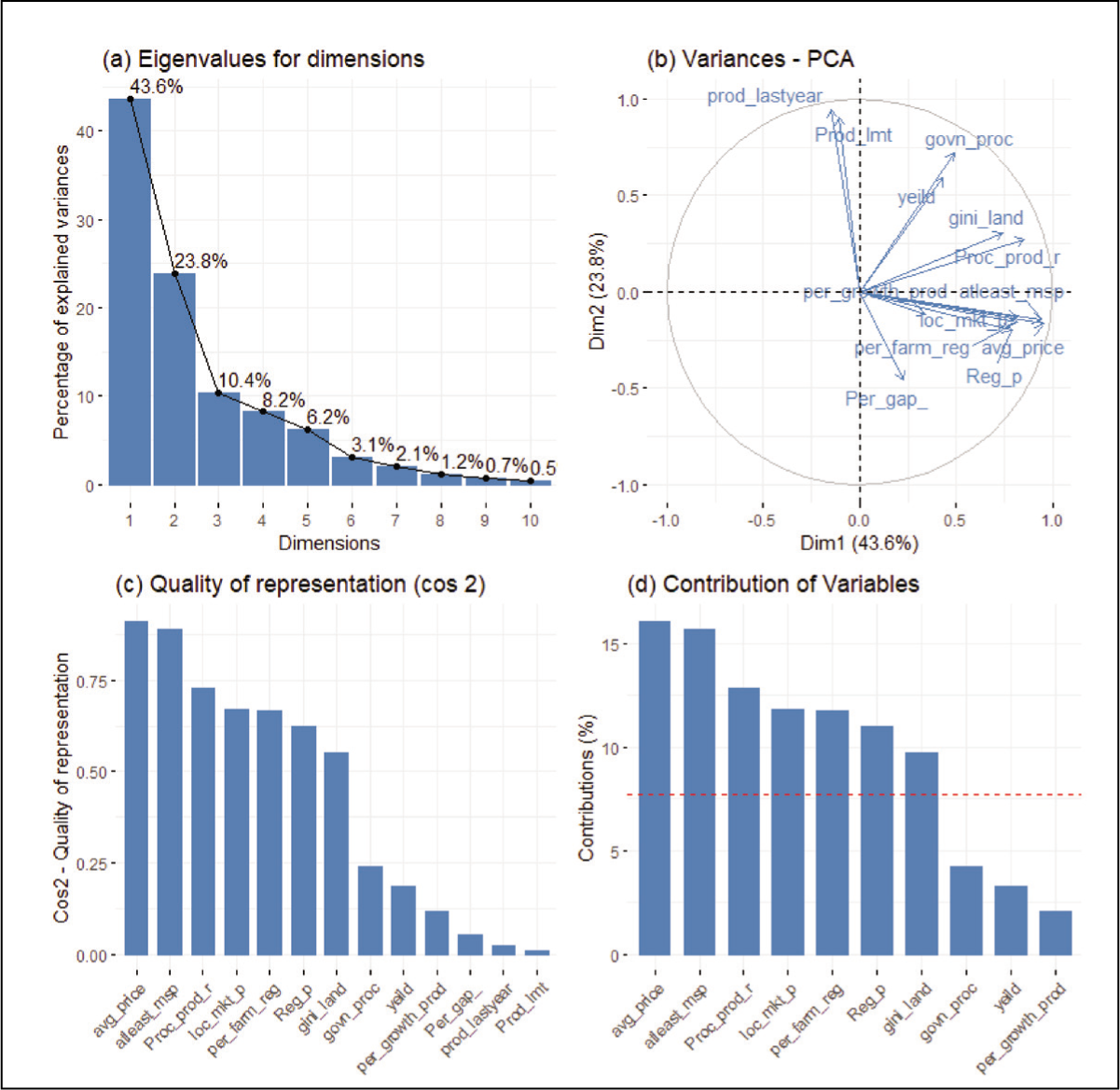
Some of the common factors affecting prices are considered in this PCM model. Factors which are expected to affect price such as production in the current year, production in the previous year, and percentage change in the production in the current year are taken in the PCM model for the dimension test. Furthermore, yield is a good proxy of better agricultural conditions, including the level of irrigation, soil suitability, better input use, etc. Regions with better yield are generally agriculturally developed regions and, therefore, agricultural markets are expected to be more developed with lesser price distortions. Thus, yield of various states is also taken as one of the possible factors affecting prices (Figure 5). Furthermore, from the demand side, government procurement and related factors, such as government procurement in quantities, and in terms of percentage of total production of the respective states, are included in the PCM model. As we have seen in the previous section, price offered in the regulated market is often higher than the market price. Therefore, percentage of farmers selling in the regulated markets and percentage of total quantity sold by farmers out of total procurement are expected to be affecting average prices. Thus, a few additional factors could be responsible for state-level variation in prices and are thus included for checking of dimensions in the model. Furthermore, not all categories of farmers have the same bargaining power to get the same prices, and it is mostly observed that bargaining power in the market has some relation with land ownership. Thus, the Gini coefficient of operational land under the cultivation is also considered as one of the possible factors affecting average price.

PCM results show that the first three dimensions contribute nearly 78% of total variation in the data, out of which the price-related variation (dimension one) is contributing to more than 43% of total variation. The second-dimension concerns primarily output- and procurement-related variables which remain outside the ambit of this paper. The third dimension also points towards the relationship between change in output, yield and percentage of farmers selling in the regulated market along with local market prices (Table 6 and Figure 6). However, for the purpose of analyzing price variation across states, dimension one is sufficient, as most of these factors are already part of the first dimension. Thus, dimension one shows that if prices are changing across states, then what are the factors also changing their values. However, change in value can be a coincidence as well, therefore the next section will explore to what extent such factors are related to each other. Once dimension one is selected, it becomes clear that some factors, such as government procurement in absolute quantity, yield, production both current and previous year, change in production, percentage of quantity sold by farmers out of total government procurement, are reflecting insignificant contribution in the dimension showing price variation (Table 5). Thus, after dimension reduction, the important factors contributing to the price dimension are identified and these factors are: percentage of government procurement out of total production of the state; percentage of farmers selling in the regulated market; Gini coefficient of land; percentage of farmers getting at least MSP price and price variables such as average price received by farmers; average price received by farmers in the regulated markets; average price received by farmers in the local markets.
Contribution of Factors in Different Dimensions in PCM.

Based on these selected factors there seems to be an existence of clusters of states. Figure 7 shows a dendrogram reflecting clusters of states in terms of these factors. All these factors are very high in states such as Punjab, Haryana, Chhattisgarh, Telangana, and Kerala. In other words, these states reflect strong presence of states in terms of procurement of paddy and a large proportion of farmers are selling in the regulated markets. These farmers also witness relatively higher average prices, both in regulated markets and local markets. Furthermore, the proportion of farmers receiving at least MSP has been very high for these states. On the contrary, all price-related variables are comparatively lower in the other two clusters (Figure 7) of states with relatively lower presence of states. Presence of clear clusters in terms of government procurement and price of paddy received by farmers across states evidently indicates the prevalence of a strong relationship between government procurement and price variation across states. For further exploration, we need to understand how different factors are correlated to each other and how various indicators related to price across states are influenced by these factors. The following section deals with the pair-wise correlation between selected factors to understand the relational aspects of the price variation across states.

Understanding Relational Aspects of Price Variations Across State
Once we select factors which are changing their values across states with the change in the price variables it is imperative to understand the nature of such relation. The correlation matrix (Figure 8) shows some very interesting relationships between the different pairs of factors. In order to understand the relational aspect and direction of such relationship, it is important to identify the set of exogenous variables. Here, production of paddy in any year in any state is largely an exogenous variable. Besides, even with year-to-year fluctuation in output, the relative position of states in terms of share in total national output remains largely stable. Furthermore, total public procurement, which is largely the outcome of political economic factors involving both center and state, and hardly changes in a short span of time, can be treated as an exogenous variable during any year. Besides, change in the procurement status for different states remains largely stable, subject to a given political-economic condition. Therefore, the procurement production ratio in any state in the model is considered as an exogenous variable for any short span of time. Furthermore, percentage of farmers selling in the regulated markets depends largely on the efficiency and inclusivity of the state’s procurement mechanism and it improves only over a time. Thus, here in the model, this ratio is treated as an exogenous variable. Furthermore, yield is here considered as a proxy of the level of infrastructure in the agriculture sector and is exogenous. Also, Gini of land is the outcome of historical process and changes very slowly over the years and, therefore, in this model, it is considered as an independent variable. Here, the case of regulated price is interesting. Though the average regulated price in all states is not the same as the MSP because of variety of reasons such as administrative inefficiencies, differential bargaining power of different stakeholders, and corruption in the procurement system, etc., the MSP has been instrumental in the determination of the regulated prices in all types of procurement agencies. As mentioned earlier, in the majority of the states, average regulated prices were observed to be higher than the market price, primarily because the MSP which is the guiding principles of regulated market has been significantly higher than the local market prices for most of the states. Thus, average regulated price has both exogenous and endogenous characteristics. Thus, the correlation matrix (Figure 8) will be explained on the basis of the impact of exogenous variables on factors such as local market prices, average prices, and percentage of farmers receiving at least the MSP.
Correlation Matrix for Various Price Related Variable.
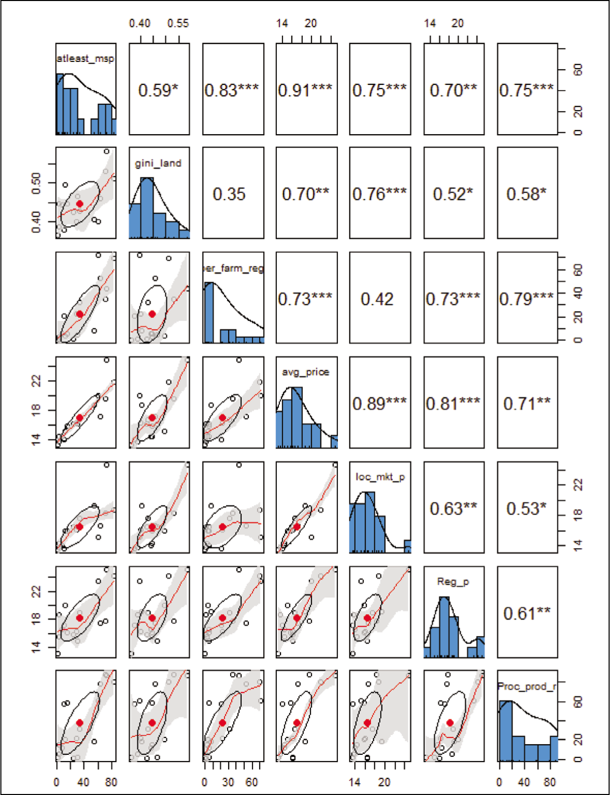
As far as the major determinants of price variation across states are concerned, government procurement remains extremely important. The average price is highly correlated with government procurement as a percentage of total production (Figure 8). Thus, states with higher procurement output ratios reflect higher average prices. Furthermore, the percentage of farmers selling in the regulated market also affects price variation positively. States with a higher proportion of farmers selling in the regulated market are showing relatively higher prices. The correla- tion coefficient between average price and percentage of farmers selling in the regulated markets is higher as well as significant. In fact, both govern- ment procurement as a proportion of total production and percentage of farmers selling in the regulated markets are highly correlated to the percentage of farmers receiving at least MSP.
Interestingly, the local market prices, which are largely market-driven, are found to be highly correlated with government procure- ment as a proportion of output. It indicates two important aspects of the relationship between market price and government procure- ment. First, the state with higher proportional procurement indicates better implementation of MSP prices and, therefore, the possibility of convergence of market prices towards regulated prices is higher. Since relative procurement across states does not vary substantially over the years, the impact of such procurement can be seen in the longer term. Thus, states with higher relative procurement reflect a lower gap between MSP and market price (or local market price). There has been strong positive relationship between average price in the regulated market and local market price. Thus, if states have higher presence in terms of procurement, the local market price tends to converse towards regulated price. Since the regulated prices have been higher than the local market prices for most of the states, higher average prices are observed in the states with higher procurement. Second, even though the correlation between local market price is not significant 11 with the percentage of farmers selling in the regulated market, the direction of relation is indicative of the same story. Thus, higher procurement at relatively higher price tends to raise the average local market price in the upward direction, and this could be through additional demand creation. 12 In other words, the tendency of convergence of local market price to the regulated price observed for states where government procurement as a percentage of total production and percentage of farmers selling in the regulated market is relatively higher (Table 7 and Figure 9).
The Average Rate of Paddy Received by Farmers from Various Procurement Agencies.


Here the case of Bihar is interesting. The state abolished the APMC Act in 2006, expecting to provide more space to private players in the agriculture markets. However, this led to the excessive dependence of farmers on local markets for procurement, and in the absence of significant government procurement, the average price (also local market price) received by farmers in the state remains much lower than the MSP and the proportion of farmers getting at least MSP has been one of the lowest in the country. Thus, the abolition of the APMC Act hardly had any positive impact on the status of farmers in terms of access to better prices of their produce in Bihar. In fact, it is interesting to observe that for some neighboring states like UP, Jharkhand, and MP, where direct government procurement has not been substantial, the APMC markets had been playing an important role and offered the highest average prices to farmers than any other agencies (Table 7). But unlike these states, with the abolition of APMC markets, the farmers in Bihar have lost one of the most important procurement agencies to offer higher prices. Since private agencies also participate in the APMC market, there is a possibility that a significant part of the private traders would have sold their produce in the APMC market at MSP which has been much higher than the prevailing market price in Bihar. Such transactions at higher prices could have put upward pressure on local market prices as well. Therefore, it is likely that the abolition of APMC in Bihar had pushed the market prices downwards as the state lost an important platform to offer higher than market prices for agricultural produce.
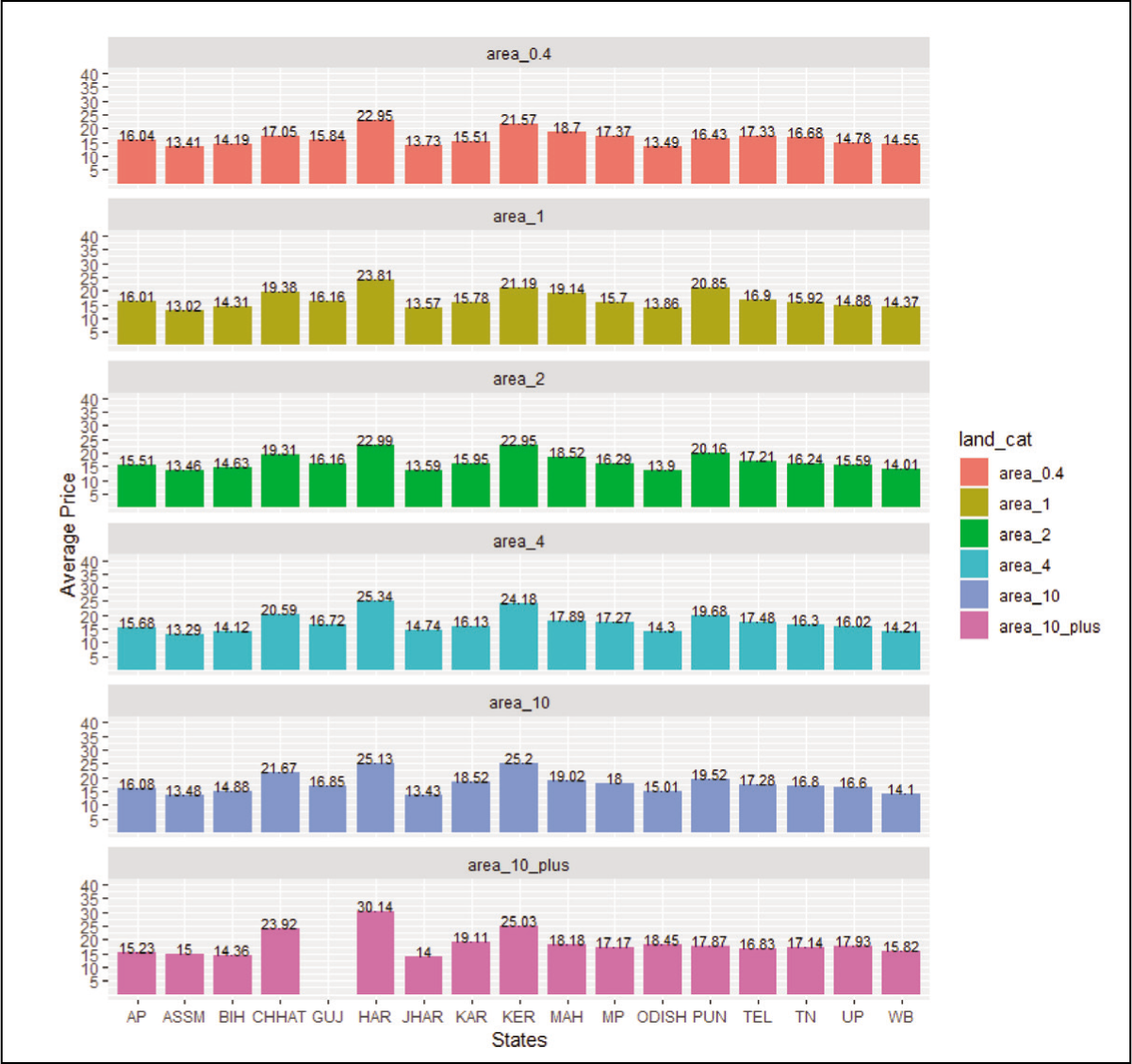
In Figure 8, average price shows a positive relation to the Gini coefficient of operational land. In fact, all price variables, such as average price, average price in the regulated market, average local market price, and percentage of farmers receiving at least MSP, are highly correlated with the Gini coefficient of land. This implies that the larger the concentration of lands, the bigger the possibility of receiving higher prices in general. It indicates that larger farmers are having better bargaining powers in terms of receiving higher prices, both in the local as well as in the regulated markets. This, in turn, leads to a higher percentage of farmers receiving MSP with more concentration of land. This is clear from Figure 10 that, for the entire country as whole, the average price received by farmers are regressive in nature. In most of the states, larger farmers are receiving higher average prices in general. In fact, Kumar et al. (2022) also find a very strong positive relationship between farm size and average price received by farmers in states like UP, Bihar, Jharkhand, Odisha, and West Bengal. It seems plausible that the bargaining power of the large farmers in the local market is higher primarily because of higher socioeconomic status of large farmers and thereby historically having better terms with the representatives of various procurement agencies. Also, since the price at the time of harvest is generally low, those farmers who could hold their produce for some time usually receive higher prices. Evidently, it is likely that large farmers with better liquidity have a better capacity to hold selling for some time and are therefore expected to get higher prices. As far as regulated market is concerned, the access to regulated market has been higher for larger farmers as compared to all small categories of farmers (Table 8). In fact, in the smallest categories of farmers (up to 0.4 acres) only 8.75% of farmers are reported to sell in the regulated markets, while this ratio goes as high as more than 46% for farmers with more than 10 acres of land. Since regulated the market offers higher prices, large farmers in general receive higher prices. Furthermore, even in the regulated markets, except for direct government procurement, the larger farmers are successful in bargaining for higher prices. This trend is true for most of the states except Maharashtra and Punjab. A possible explanation for such a trend is that breaks in both states might be due to the presence of a strong farmers’ lobby, proximity to big cities, and cultivation of high values paddy (like Basmati particularly in case of Punjab under contract farming). While higher bargaining power of large farmers in the local market is expected, the presence of such a trend in the regulated market is somewhat worrisome, as one of the objectives of public procurement has been to provide affordable prices to all farmers and, more importantly, to ensure inclusivity to small and marginal farmers.
Land Size and Procurement Agencies.

Conclusion
The average price received by farmers has been different across states, and the major correlate of such difference in prices has been the share of government procurement as a proportion of output of the state, along with the inclusiveness of government procurement in terms of percentage of farmers selling in the regulated markets. The average price in the regulated markets has been higher as compared to local market prices, except for some states. There is also evidence of conversion of local market price towards average regulated market price for states in which government procurement has been higher as a percentage of total production and procurement is largely happening directly from the farmers. Thus, variation in prices across states both in the regulated and non-regulated market is highly correlated with the degree of government intervention in the procurement. Thus, with higher government procurement, farmers on average receive higher prices primarily on two accounts: first, average price in the regulated market is higher than the local market, and, therefore, higher access to regulated markets gives farmers direct access to higher prices; second, marking an indirect effect, higher procurement puts upward pressure on local market price as well. So even if farmers are unable to sell their produce in the regulated markets, they get relatively higher prices in local markets in states having a higher procurement production ratio.
Thus, one may infer that if government procurement through MSP is reduced or done away with to rely more on competitive markets, there is a strong possibility that the market price for crops like paddy would collapse and the situation would deteriorate further. 13 Given the fact that an overwhelming proportion of farmers are not receiving remunerative prices for their products, withdrawal or weakening of public procurement system might unleash forces responsible for dispossession of farmers with the deepening of agrarian crises and can accelerate the process of primitive accumulation through displacement as has been evident in case of Africa (Moyo et al., 2014). The role of landownership has also been important in this regard, and the evidence shows that not only in the non-regulated markets but also in the regulated markets, larger farmers are better placed in terms of bargaining for a higher price. In regulated markets, it is indeed a matter of concern and must be addressed through proper channels. Nevertheless, it is quite evident from the data that, for all small categories of farmers, regulated markets undisputedly offer higher prices than all the other forms of non-regulated markets across states.
Thus, withdrawal of the state in terms of lower public procurement would harm small and marginal farmers with lower bargaining power in the local markets and there would also be the lowering/absence of upward pressure on local market prices that arises due to the public procurement system in India. In fact, what seems essential for “doubling” farmers’ incomes at the current juncture is rather to strengthen the public procurement systems in the country along with correcting its large farmer and regional biases.
Footnotes
Declaration of Conflicting Interests
The author declared no potential conflicts of interest with respect to the research, authorship, and/or publication of this article.
Funding
The author received no financial support for the research, authorship, and/or publication of this article.