State Fiscal Capacity and Tax Effort: Evidence for Indian States

Abstract

This study analyzes the tax effort of 17 Indian states as a means of creating fiscal space. Four individual state-level taxes—stamp duty and registration fees, state sales tax, state excise duty and motor vehicles tax—are studied as well as the total own-tax revenue of states. Stochastic frontier analysis (SFA) models have been estimated for each of the taxes and for own-tax revenue in order to obtain a measure of inefficiency in tax collection. The data used for the SFA models span the time period 2000–2001 to 2010–2011. The results of the estimation exercises point to technical inefficiency as being the primary reason for states being unable to achieve their potential for revenue collection. Possible reasons for this inefficiency are examined. The estimated tax effort points to large budgetary room that states potentially enjoy for the purpose of raising revenues from existing taxes. Rather disconcertingly, the article notes that the average tax effort seems to be declining over time.

JEL Classification: H21, H71

Keywords

Tax effort stochastic frontier analysis fiscal capacity

Introduction

The term ‘fiscal space’ has been used in various contexts and has been invested with different connotations. There is the standard IMF connotation which defined it as ‘room in a government’s budget that allows it to provide resources for a desired purpose without jeopardizing the sustainability of its financial position or the stability of the economy’ (Heller, 2005b). Even within the IMF there is a difference in emphasis. Ostry, Ghosh, Kim and Qureshi (2010) define fiscal space as the ‘difference between the current level of public debt and the debt limit implied by the country’s historical record of fiscal adjustment’. Aizenman and Jinjarak (2010) seek to make Heller’s (2005a, 2015b) definition precisely measurable by proposing the concept of de facto fiscal space: de facto fiscal space is defined as being inversely related to the tax-years it would take to repay the public debt. The Organisation for Economic Co-operation and Development (OECD) has a similar approach to the concept. Schik (2009) describes it as financial resources available to a government for policy initiatives through the budget and related decisions without prejudicing sustainability of its fiscal position. The approaches described thus far, according to Roy, Heuty and Letouzé (2007), view fiscal space in residual terms and are concerned with short-run consequences of an increase in public expenditures. Roy et al. (2007) are, on the other hand, concerned with making resources available for long-term goals of development.

Our approach in this article is more attuned to that of Heller (2005a, 2005b). Without denying the importance of long-term developmental issues, our concern is with respect to short-run finances of governments. Our focus will be on finances of state governments in India which face serious challenges in terms of expanding the fiscal space available to them for the purpose of discharging their duties. Important issues that crop up in this context are: ability and capacity of governments to raise tax and other revenues; reprioritizing expenditures; and funding from the federal government. Our focus will be on the first of these, namely, evaluating the capacity of governments to raise tax revenues and, obliquely, also on funding from federal government.

It has often been pointed out that Indian states have not striven enough to raise sufficient tax revenues and thereby boost their tax effort. The review section discusses some of these studies in more detail. There are two factors at work here: the first is the effort of state governments towards boosting revenue collection being stymied by the absence of adequate tax bases; the second is the inability of governments to exploit their existing tax bases adequately. Our exercises in this article will have something to say about the inadequate exploitation of tax bases by Indian states.

The context in which we examine the inability of state governments to raise tax revenues is the Indian federal system which has three tiers of government: the central or federal government, the state governments and the local governments comprising rural and urban local bodies. There exists a serious imbalance in the distribution of revenue collecting powers between the federal government and the other levels of government. The Indian Constitution does provide for a distribution of powers and responsibilities of the federal and state governments. These are listed in the Union (federal), State and Concurrent lists in the seventh schedule of the Indian Constitution. While there is precision in the items listed in the Union and State lists, the federal government can override the states on the concurrent list and residuary powers are also assigned to it. There is criticism that India is a federation only in name while in reality the distribution of powers is skewed in favour of the federal government.

A distinguishing feature of the Indian federation is the uneven distribution of tax bases to the various levels of government. The state (and local) governments have been left with tax bases that do not generate adequate revenues, which inevitably fall short of the expenditure responsibilities that have been placed on them (Rao, 2005). Recognising the weak revenue–expenditure position of the states, the Indian Constitution has provided for the setting up of a Finance Commission every five years. The functions of the Commission include (Rao, 2000):

Distribution of the proceeds from taxes which are to be shared between the federal and state governments.

Provision of grants-in-aid to states in need of assistance.

Measures to augment resources of state governments to supplement the resources of local governments.

Address any other matter referred to the Commission in the interest of sound finance.

In addition to the Finance Commissions, the Indian Planning Commission also provides substantial assistance in the form of loans and grants for financing the development plans of states (Planning Commission, 2012). Loans and grants are given in the ratio 70:30 for states in the non-special category, while this ratio is 10:90 for ‘special category³ states. The final source of funding to states is through federal ministries. These are of two schemes under this source: central (or federal) schemes which are entirely funded by the federal government and centrally sponsored schemes which involve sharing of costs between the federal government and the states (Rao, 2000).

Apart from the assistance that states receive from the federal government, they also have been striving through their own efforts to expand the fiscal space available to them through rationalization of expenditures as well as through revenue augmentation. These efforts of the states have led to some successes. For instance, committed expenditures (comprising expenditures on interest payments, administrative services and pensions) of the non-special category states has shown a marginal decline from an average of 5 per cent of gross state domestic product (GSDP) over 2000–2005 to 4.5 per cent of GSDP in 2011–2012. More specifically, expenditure on wages and salaries as a percentage of GDP has declined from an average of 4.11 per cent in 2000–2001 to 2004–2005 to 2.99 per cent of GDP in 2011–2012. Likewise, non-development expenditure of states has also declined from 35.16 per cent of total expenditure in 2000–2001 to 2004–2005 to 28.84 per cent of total expenditure in 2011–2012. States have simultaneously, also focused on revenue augmentation through broadening and rationalizing their tax systems, improving the efficiency of their tax administration, simplification of their tax laws and better compliance. States’ own-tax revenues (OTR) as a ratio to GSDP have increased from 5.83 per cent during 2000–2001 to 2004–2005 to 6.6 per cent in 2011–2012. Despite these commendable efforts of the states, our article will show serious inefficiencies in tax collection leading to poor tax effort.

This article seeks to contribute to the literature on tax effort (and the associated fiscal capacity) by employing stochastic frontier analysis (SFA) to measure tax revenue performance of four important taxes—stamp duty and registration fees, state sales tax, state excise duty on alcoholic beverages and motor vehicles tax (inclusive of taxes on vehicles and taxes on goods and passengers)—of 17 non-special category states. It may be noted that the seventeen non-special category states considered in the article together account for nearly 95 per cent of India’s population, enjoy similar fiscal arrangements under the Constitution and also traverse the space of high-, middle- and low-income states. The plan of this article is as follows: the second section provides a review of prior research in estimating tax effort; the third section discusses the methodology adopted in this article; the fourth section presents our estimated SFA models; the fifth section seeks to identify the factors responsible for the inefficiencies in tax collection identified by our SFA models; the sixth section estimates the tax effort of states; the seventh section concludes.

Estimating Tax Effort: A Review of Prior Research

In this article we are concerned with examining the ability and efficiency of states in raising tax revenues. The tax effort of states can be viewed as a self-help process whereby efforts are made to mobilize additional revenues as the economy grows and taxable capacity expands. Tax effort may be enhanced by the introduction of new taxes, changes in the rates and bases of existing taxes, and improvement in tax administration and collection. Various institutional changes have also been proposed to encourage states to enhance their tax effort. Finance Commissions have sought to encourage states to increase their tax effort by devising formulas for tax sharing that reward states with superior tax effort (Government of India, 2015). Likewise, the Planning Commission too, employing the Gadgil and modified-Gadgil formulae to allocate federal funds to states, gives importance to the tax effort of the states (Mohan & Shyjan, 2009). Numerous studies have been carried out to estimate the tax effort for India as well as other countries. We first look at studies in other countries before turning to India.

Three papers—Davoodi and Grigorian (2007), Sobarzo (2004) and Stotsky and Woldemariam (1997)—are concerned with estimating tax effort of countries without delving into the inefficiencies that militate against improvement in this effort. Stotsky and Woldemariam examine the determinants of the tax share in GDP and construct a measure of tax effort using panel data analysis for 43 sub-Saharan African countries for the period 1990–1995. Their main finding is that the share of agriculture and mining in GDP is inversely related to the tax share in GDP. Sobarzo studies the tax effort and tax potential of state governments in Mexico, finding that revenue-raising capacity was highly skewed in favour of the central government and state governments depended heavily on transfers from the central government. Davoodi and Grigorian examine the determinants of tax potential for Armenia and extend the analysis away from the conventional approach by including measures of institutional quality and shadow economy in a panel data framework for the period 1994–2004. The study finds that improvements in institutional quality and reduction in the size of the shadow economy play a major role in improving tax performance.

The next two studies adopt the approach that we have employed in this article. Alfirman (2003) estimates the stochastic frontier tax potential for Indonesian local governments. The paper finds that, after decentralization, Indonesian local governments would have to exploit existing revenue potential rather than impose additional taxes to improve revenues. Fenochietto and Pessino (2013) also employ the same technique using panel data to estimate tax effort for 113 countries. The paper finds that high per capita GDP, high education levels, open economies, low inflation, low corruption and strong policies of income distribution lead to greater efficiency in tax collection.

The Indian studies that we report concentrate on estimating tax effort of Indian states. However, most of these studies confine their attention to merely estimating tax effort without seeking to determine the possible reasons for the low tax effort. Specifically, no attempt is made to distinguish between limitations imposed by the inadequacy of appropriate tax bases on the one hand and the inability to exploit existing taxes adequately.

One of the earliest studies on the subject is Reddy (1975) which analyzed the relative tax effort for 16 states over the period 1970–1972. Three ratios were employed in the analysis: state own-tax revenue–income ratio, states’ own tax plus non-tax revenue–income ratio and states’ own tax and non-tax revenue as a percentage of state’s income net of taxes paid to the centre. The paper finds that the method of computing tax effort of states needs improvement and that the tax–income ratio should be refined to account for differences in income among states, the structure of income distribution as well as others factors which influence taxable capacity.

Oommen (1987) studied the relative tax effort of 16 states using two measures of tax effort, namely, the tax–income ratio, and elasticity and buoyancy of tax revenue. The paper employs a stepwise regression approach to estimate tax to income ratio for data of 16 states pooled over 1970–1971 to 1981–1982. Once the equation is estimated, state-specific values are plugged in to the right hand side to obtain the presumptive tax effort for each state. Southern states were seen to display much superior tax effort while the effort of some of the richer states has been poor.

Sen (1997) studied the relative tax effort of the 15 non-special category states for the time period 1991–1992 to 1993–1994 estimating separate cross-section regressions for each of the taxes at the state-level as well as for the aggregate of all taxes. It was found that performance on the aggregate tax effort index was largely influenced by the tax effort for sales tax given its large share in own tax revenue of the states.

Coondoo, Majumdar, Mukherjee and Neogi (2001) analyzed the relative tax performance for 16 states for the period 1986–1987 to 1996–1997 using quantile regression analysis and examined whether and how the ordinal position of individual states’ tax–SDP ratio changes over time. The analysis revealed that the southern and western states showed superior tax performance over the other states which may be attributed to relatively larger taxable capacity, relatively greater tax effort or certain political–economic characteristics.

Purohit (2006) studied the tax effort and taxable capacity of both the federal government and 16 state governments for the period 2000–2003. The paper considered all taxes at the state level, calculated the tax effort for each state and found that Gujarat ranked first in tax effort. Tax effort of the federal (central) government, on the other hand, was examined using macroeconomic variables and the regression approach.

The Reserve Bank of India (2013) studied the tax effort of individual states by carrying out a state-wise analysis of tax buoyancy for OTR of a state as well as for major state-level taxes for two time periods 2000–2004 and 2004–2008. The period 2004–2008 witnessed significant fiscal consolidation and it was observed that OTR buoyancy was lower for 13 of the 17 states during the fiscal consolidation period 2004–2008 as compared to 2000–2004. The study further pointed out that OTR buoyancies for the years 2010–2011 to 2012–2013 showed an improvement over the fiscal consolidation period in 14 of the 17 states.

Garg, Goyal and Pal (2014) employ SFA to study the tax capacity and tax effort of own-tax revenues of the 14 major states for the period 1991–1992 to 2010–2011. The paper seeks to answer questions such as the role of economic structure on tax capacity of the states, the impact of federal transfers, implementation of the fiscal responsibility legislation and the political environment, including governance, on the tax effort of a state. The paper finds that while per capita GSDP has a significant positive impact, the size of the agricultural sector has an adverse impact on states’ own-tax revenue.

The approach that we employ in this paper goes well beyond estimating tax efforts of Indian states as has been done by most studies in India. We seek to investigate whether any inefficiency exists in the tax collection efforts of the states. We do this separately for four state level taxes as well as for OTR of states. Should such inefficiency exist, we propose to understand the reasons for these inefficiencies.

Methodology

Tax performance for any level of government is usually measured by the ratio of actual performance to a measure of taxable capacity, such as the tax–GSDP ratio. Apart from being a simple indicator of performance, GSDP could well be an imperfect proxy for the tax base particularly when the tax structure comprises of different taxes, each of which is related to a distinct tax base. Consequently, estimation of tax effort and taxable capacity requires the use of appropriate proxies of the tax base and estimation procedures different from the mere computation of this simple tax–GSDP ratio. The literature points towards two techniques for the purpose of estimating tax effort based on the disaggregated performance of individual taxes. The standard techniques employed are the regression approach (RA) and the representative tax system (RTS) approach.

The RA uses multivariate regression analysis to explain the variation in tax performance across different units (either countries or states within a country), using a set of regressors which best proxy the tax bases. Tax effort is computed by taking the ratio of the actual revenue performance to the predicted values from the regression equation (Sen, 1997). When the predicted value equals the actual revenue collections, the ratio equals one and the unit has little room for improvement. But when the ratio is less than one, revenue collections lie below the predicted values and improvement the collections can expand the fiscal space. RTS, popularly used in the federal set-up of the United States and Canada, ‘links major state and local tax collections to their ideal or standardized bases and calculates what revenue each state could generate from these ideal bases if the nationally representative rate were levied’ (Mikesell, 2007). In this method, instead of taking proxies for potential tax bases, an appropriate base is identified and a representative of tax rate is generated for every tax. The effective rate of a tax is the ratio of actual tax revenue to the potential base of the tax. The tax effort of a particular state is nothing but the ratio of actual tax revenue obtained by the state and its taxable capacity (Purohit, 2006).

Stochastic frontier analysis (SFA) is employed in this article to estimate the tax frontier and, based on it, the tax potential for 17 Indian states are estimated. The tax frontier for a particular tax is a function that expresses the maximum amount of tax that can be collected from a given tax base. Stochastic frontier models were first developed by Aigner, Lovell and Schmidt (1977) and have been increasingly used in efficiency analysis. Extensions of the stochastic frontier models from cross-section data to panel data have followed Pitt and Lee (1981).

Suppose a producer has a production function f( x _i , a). In a world with no inefficiency, the firm i would produce

y_{i} = f (x_{i}, a)

(1)

where

y_i = output

x _i = vector of inputs

a = vector of parameters to be estimated.

A fundamental element of SFA is that each firm can potentially produce less than its maximum capacity due to inefficiency which renders the production function as:

y_{i} = f (x_{i}, a) + e_{i} i = 1 ..... N

(2)

where,

e_i = v_i – u_i, is a composite of two error terms:

v_i is a normally distributed error term representing measurement and specification error or noise and represents factors beyond the control of the firm; $v_{i} \sim N (0, σ_{v}^{2})$

u_i is a one-sided error term which represents inefficiency, that is, the inability to produce the maximum level of output given the inputs used. The component u_i is assumed to be distributed independently of v_i and to satisfy u_i ≥ 0. The non-negativity of the technical inefficiency term reflects the fact that if u_i > 0 the unit (firm or country or state) will not produce at the maximum attainable level. The generalisation of the specification of u_i by Battese and Coelli (1988) is given by $u_{i} \sim N^{+} (0, σ_{u}^{2})$ or $u_{i} \sim N^{+} (μ, σ_{u}^{2}) .$

The panel data variant for the SFA model may be written in log form as:

\ln (y_{i t}) = β_{0} + \sum_{j = 1}^{k} β_{j} \ln (x_{j i t}) + v_{i t} - u_{i t}

(3)

where, v_it is the idiosyncratic error and u_it is a time varying panel level effect. The simplest specification of the SFA model is the time invariant inefficiency model where u_it is a time invariant truncated normal random variable. In such a model, $u_{i t} = u_{i}, u_{i} \sim i i d N^{+} (μ, σ_{u}^{2})$ and $v_{i t} \sim i i d N (0, σ_{u}^{2}) .$ u_it and v_it are distributed independently of each other and the covariates in the model.

In empirical estimations involving long panel data sets, the plausibility of time invariant inefficiency term has been questioned and an alternative time-varying decay model is proposed. In what follows, we have employed the time-invariant inefficiency approach because our panel data set is not particularly long and these models yielded better results.

A measure of inefficiency can be obtained by means of the parameter γ which is defined as

γ = \frac{σ_{u}^{2}}{σ_{u}^{2} + σ_{v}^{2}}

(4)

where, $σ_{v}^{2}$ and $σ_{u}^{2}$ are the variances of the noise and inefficiency effects, respectively.

The value of γ lies between 0 and 1. If it is close to zero then deviations from the frontier can be attributed to noise, while, if the value of γ is close to 1, then deviations from the frontier can be attributed to technical inefficiency (Battese & Corra, 1977; Coelli, Rao, O’Donell & Battese, 2005; Tran, Grafton & Kompas, 2008).

Empirical Evidence

We now begin our analysis of the tax effort of Indian states and assess their tax potential for the period 2000–2001 to 2010–2011. We will estimate the efficiency of states in raising revenues from state-level taxes. The decade 2000–2001 to 2010–2011 is divided into two sub-periods, namely, 2000–2001 to 2004–2005 and 2005–2006 to 2010–2011 for purposes of comparison. These two time periods more or less coincide with the award period of the Eleventh Finance Commission (2000–2001 to 2004–2005) and the Twelfth Finance Commission (2005–2006 to 2010–2011). We present our results in two parts. In the first, we look at the data for Indian states and try to identify some trends. In the second part, we report results of the stochastic frontier analysis.

Preliminary Examination of the Data

The 17 non-special category states that we consider are: Andhra Pradesh, Bihar, Chhattisgarh, Goa, Gujarat, Haryana, Jharkhand, Karnataka, Kerala, Madhya Pradesh, Maharashtra, Orissa, Punjab, Rajasthan, Tamil Nadu, Uttar Pradesh and West Bengal. The four major taxes of these states that we focus on are given below while the details about each tax are given in the relevant sub-section when we estimate the SFA model.

Stamp duty and registration fees.

State sales tax (replaced by value added tax [VAT] from 2005).

State excise duty on alcoholic beverages.

Motor vehicles tax (motor vehicles tax comprises of taxes on vehicles and taxes on goods and passengers).

In addition, we also consider the OTR of each state. OTR is a good indicator of the tax performance of a state since it is computed excluding any allocations that maybe made by the federal government to a state. Table 1 gives information on OTR as a percentage of GSDP of the state and as a percentage of its total tax revenues. We present this separately for the two sub-periods.

Table 1 compares the average OTR/GSDP ratio for the seventeen non-special category states for the two sub-periods and we find that the average OTR/GSDP ratio for these states together has shown a marginal increase from 6.34 per cent (2000–2001 to 2004–2005) to 6.65 per cent (2005–2006 to 2010–2011). A comparison of the ratio across the two sub-periods indicates that seven of the seventeen states have an OTR/GSDP ratio lower than the average during each of these sub-periods. States that have lower-than-average OTR/GSDP ratios during first sub-period include Bihar, Chhattisgarh, Jharkhand, Orissa, Rajasthan, Uttar Pradesh and West Bengal. During the second sub-period, there is a slight change in this set of seven states: Gujarat now exhibits a lower than average OTR/GSDP ratio whereas Chhattisgarh shows a remarkable improvement and its ratio rises from 5.63 per cent to 7.29 per cent. While the OTR/GSDP ratio shows an improvement in the latter time period, this is not the case when we consider OTR as a share of total tax revenues. The average for the 17 states has fallen by over two percentage points over the two sub-periods. Only two states—Karnataka and Orissa—have a shown a marginal improvement in their ratio while there has been deterioration for all the other states.

Table 1.

Own-Tax Revenues of States

States	% of GSDP		% of Total Tax Revenues*
States	2000–2001 to 2004–2005	2005–2006 to 2010–1011	2000–2001 to 2004–2005	2005–2006 to 2010–2011
Andhra Pradesh	7.13	7.74	74.72	73.56
Bihar	4.40	4.51	29.21	25.11
Chhattisgarh	5.63	7.29	62.24	61.04
Goa	6.89	6.92	83.83	78.40
Gujarat	6.67	6.50	85.84	81.66
Haryana	7.47	7.19	91.20	88.10
Jharkhand	3.77	5.02	49.76	47.89
Karnataka	8.54	8.11	79.16	80.39
Kerala	7.50	7.71	79.44	79.21
Madhya Pradesh	6.34	7.46	59.30	57.34
Maharashtra	7.17	6.90	89.16	86.90
Orissa	5.04	5.63	49.09	49.41
Punjab	6.70	6.97	88.66	85.06
Rajasthan	6.12	6.54	66.30	62.88
Tamil Nadu	8.29	8.48	81.96	80.68
Uttar Pradesh	5.71	5.63	52.18	49.21
West Bengal	4.38	4.38	60.39	57.67
Average	6.34	6.65	69.55	67.33

Source: Author calculations.

Note: * Inclusive of transfers from the federal government.

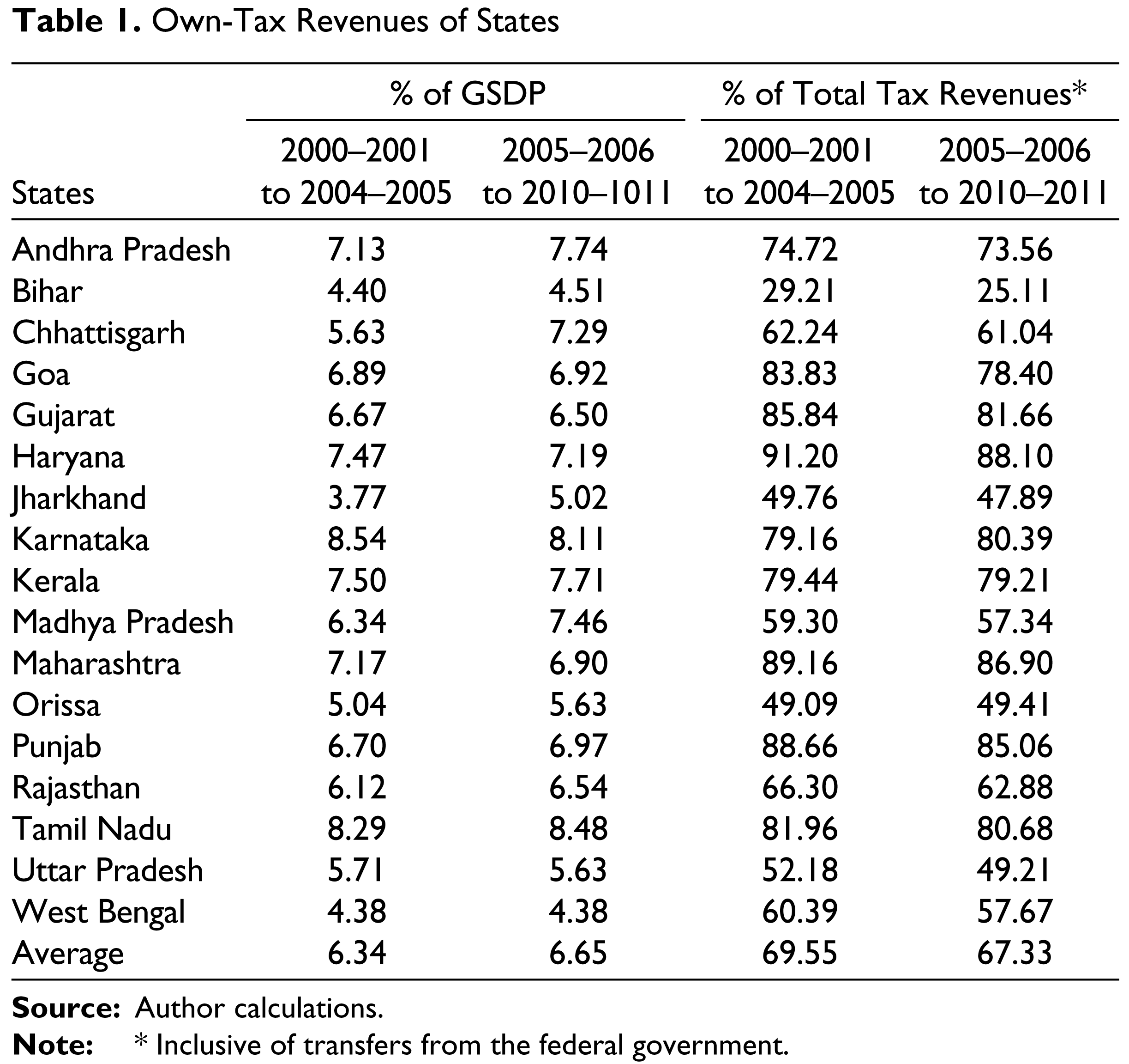
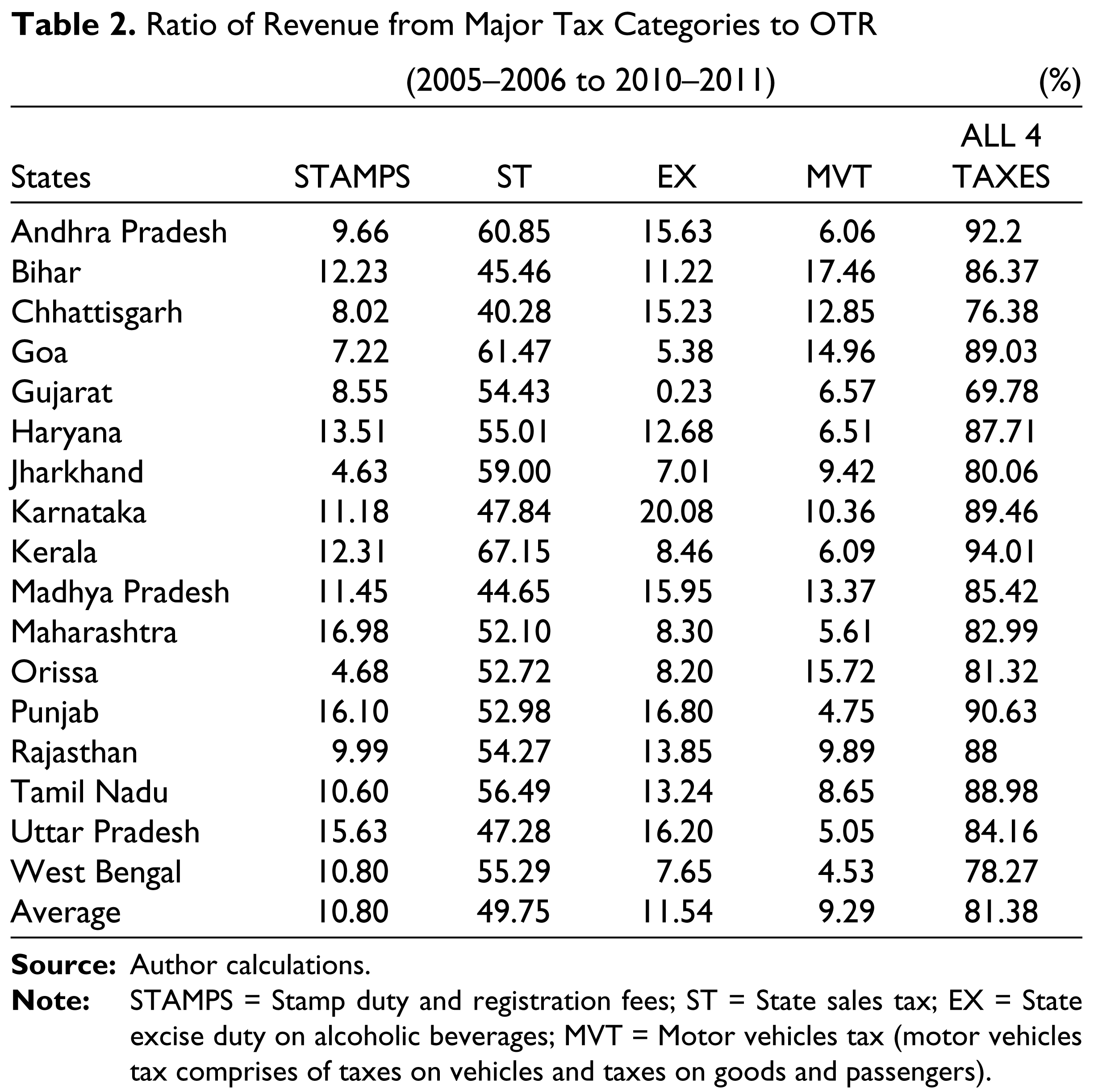
Table 2 presents a picture of the importance of the four taxes that we consider. We present this only for the second time period.

The four taxes listed in Table 2 are the biggest contributors to OTR of states. The largest contribution is from state sales tax (ranging between 40.28 per cent in Chhattisgarh to 67.15 per cent in Kerala). The next major contributor is state excise duty on alcoholic beverages, which ranges from 20 per cent in Karnataka to 0.23 per cent in Gujarat. It may be noted that the extremely low share of this tax in Gujarat is due to the policy of prohibition on sale of alcohol in the state. Collection from stamp duty and registration fees is the highest in Maharashtra at almost 17 per cent and the lowest in Jharkhand at 4.63 per cent. Finally, taxes on vehicles plus taxes on goods and passengers collect over 17 per cent of OTR in Bihar and 4.53 per cent in West Bengal. The last column of Table 2 shows the contribution of these four taxes to the total OTR of each state. On average, states are generating 81 per cent of their OTR from these four taxes with collections varying from almost 70 per cent of OTR in Gujarat to a high of 94 per cent in Kerala. For three states (Andhra Pradesh, Kerala and Punjab), this contribution is more than 90 per cent; for seven states (Bihar, Goa, Haryana, Karnataka, Madhya Pradesh, Rajasthan and Tamil Nadu), it is between 85 per cent and 90 per cent; for four states (Jharkhand, Maharashtra, Orissa and Uttar Pradesh) it is between 80 per cent and 85 per cent; and, for the remaining three states (Chhattisgarh, Gujarat and West Bengal), it is below 80 per cent.

Table 2.

Ratio of Revenue from Major Tax Categories to OTR (2005–2006 to 2010–2011) (%)

States	STAMPS	ST	EX	MVT	ALL 4 TAXES
Andhra Pradesh	9.66	60.85	15.63	6.06	92.2
Bihar	12.23	45.46	11.22	17.46	86.37
Chhattisgarh	8.02	40.28	15.23	12.85	76.38
Goa	7.22	61.47	5.38	14.96	89.03
Gujarat	8.55	54.43	0.23	6.57	69.78
Haryana	13.51	55.01	12.68	6.51	87.71
Jharkhand	4.63	59.00	7.01	9.42	80.06
Karnataka	11.18	47.84	20.08	10.36	89.46
Kerala	12.31	67.15	8.46	6.09	94.01
Madhya Pradesh	11.45	44.65	15.95	13.37	85.42
Maharashtra	16.98	52.10	8.30	5.61	82.99
Orissa	4.68	52.72	8.20	15.72	81.32
Punjab	16.10	52.98	16.80	4.75	90.63
Rajasthan	9.99	54.27	13.85	9.89	88
Tamil Nadu	10.60	56.49	13.24	8.65	88.98
Uttar Pradesh	15.63	47.28	16.20	5.05	84.16
West Bengal	10.80	55.29	7.65	4.53	78.27
Average	10.80	49.75	11.54	9.29	81.38

Source: Author calculations.

Note: STAMPS = Stamp duty and registration fees; ST = State sales tax; EX = State excise duty on alcoholic beverages; MVT = Motor vehicles tax (motor vehicles tax comprises of taxes on vehicles and taxes on goods and passengers).

Stochastic Frontier Analysis

We now turn to stochastic frontier analysis to estimate tax potential and tax effort for the major taxes and OTR. This requires that we identify a set of regressors which adequately proxy the tax bases. Our choice of regressors was guided by theory but also constrained by the availability of data.

Stamp Duty and Registration Fee (STAMPS)

STAMPS is paid to the government whenever a financial instrument or immovable property is registered at the time of purchase or transfer. The registration fee for different kinds of transactions varies. The base of the tax should ideally be the value of the property purchased or sold, data on which is, unfortunately, difficult to obtain. The proxy for the tax base is the sectoral share of construction and real estate, ownership of dwellings and business services in GSDP, which we call REALCON. We also include as regressor a variable to represent urbanization, namely, the percentage of urban population in the total population of a state (URBTOT). The rationale for this is that a significantly large number of property transactions take place in urban centres.

Table 3 presents the estimated SFA model for STAMPS. All variables used in the estimation were log-transformed. It may be noted that for each tax we estimated, both, time varying and time invariant SFA models. Our results with the time invariant option were much better and we report only these models.

Table 3.

Stochastic Frontier Analysis (STAMPS): Time-invariant Model

	2000–2001 to 2010–2011	2000–2001 to 2004–2005	2005–2006 to 2010–2011
Constant	−18.5426***(0.000)	−6.0030***(0.00)	−5.6606***(0.000)
REALCON	1.6501***(25.69)	1.3709***(0.00)	1.2503***(0.000)
URBTOT	0.8558*(0.077)	−0.0089(0.976)	0.3249(0.116)
μ	1.5862**(0.01)	1.15(1.30)	0.9808**(0.020)
γ	0.8783***	0.41	0.7476**

Source: Author calculations.

Notes: p-values are in parentheses. *** = p < 0.01; ** = p < 0.05; * = p < 0.10.

μ is the estimated mean of the truncated normal distribution.

γ is the estimate of the term in Equation (4).

The estimated equation reveals that REALCON has a positive and significant impact on the collections from this tax. URBTOT is positive in two of the three time periods but is statistically significant at almost the 8 per cent level of significance only for 2000–2001 to 2010–2011. This suggests that urbanization may not have a significant impact on collections from STAMPS. Further, the γ statistic for both, the overall period 2000–2001 to 2010–2011 and for 2005–2006 to 2010–2011, is significant at the 1 per cent and 5 per cent levels respectively, but is not significant for the first sub-period. This result indicates that the deviations from the frontier are not entirely due to noise. Inefficiency contributes almost 88 per cent to the value of γ over the entire time period and about 75 per cent during the second time period.

State Sales Tax (ST)

Revenues from ST contribute a significant percentage to own tax revenue in the states. Sales tax is an indirect tax levied when there is a sale or transfer of goods to a consumer and includes all consumer/producer goods as well as raw materials. There is no uniformity in the tax rates across states and rates are different for different categories of goods. It may be noted that 2005 onwards, sales tax was replaced by VAT. Hence, in the second time period of our analysis, the data refers to VAT collections. The sectoral share of manufacturing GSDP (MANU) is used as proxy for producer goods and raw materials sold while the annual per capita household consumption expenditure (APCE) in both rural and urban areas is proxy for final consumption. We had to exclude two states from the estimation of the SFA equation for ST: Goa and Uttar Pradesh. Data on household consumption expenditure (APCE) were not available for Goa. For Uttar Pradesh, there was a problem with the data for sales tax collected by the state in 2003–2004. For this year, amount collected is reported as ₹5.4 million by Reserve Bank of India (2010) which seems an inordinately low number given the values for one previous year (in 2002–2003, the amount was ₹6.38 billion) and one succeeding year (in 2004–2005, the amount was ₹8.88 billion). It appeared to us that this was an error in the data which we were unable to rectify from any other source. Perforce, we decided to drop Uttar Pradesh from the estimation reported in Table 4.

The results of Table 4 show that both MANU and APCE are statistically significant in all three time periods. The coefficients of both the variables are positive, as expected. The γ statistic is seen to be significant in all the three time periods. The significance of γ and the fact that it is close to unity suggests that deviations from the frontier are mainly due to technical inefficiency. Further, the fact that the value of γ has increased during the second sub-period suggests that inefficiency in tax collection has increased over time.

Table 4.

Stochastic Frontier Analysis (ST): Time-invariant Model

	2000–2001 to 2010–2011	2000–2001 to 2004–2005	2005–2006 to 2010–2011
Constant	−5.1776***(0.000)	−0.7116(0.522)	−3.2170***(0.000)
MANU	0.8092***(0.000)	0.7270***(0.000)	0.4083***(0.000)
APCE	0.6905***(0.000)	0.2763**(0.006)	0.9183***(0.000)
μ	0.6424**(0.026)	0.5883(0.119)	0.6898***(0.000)
γ	0.8642***	0.9163***	0.9352***

Source: Author calculations.

Notes: See notes to Table 3.

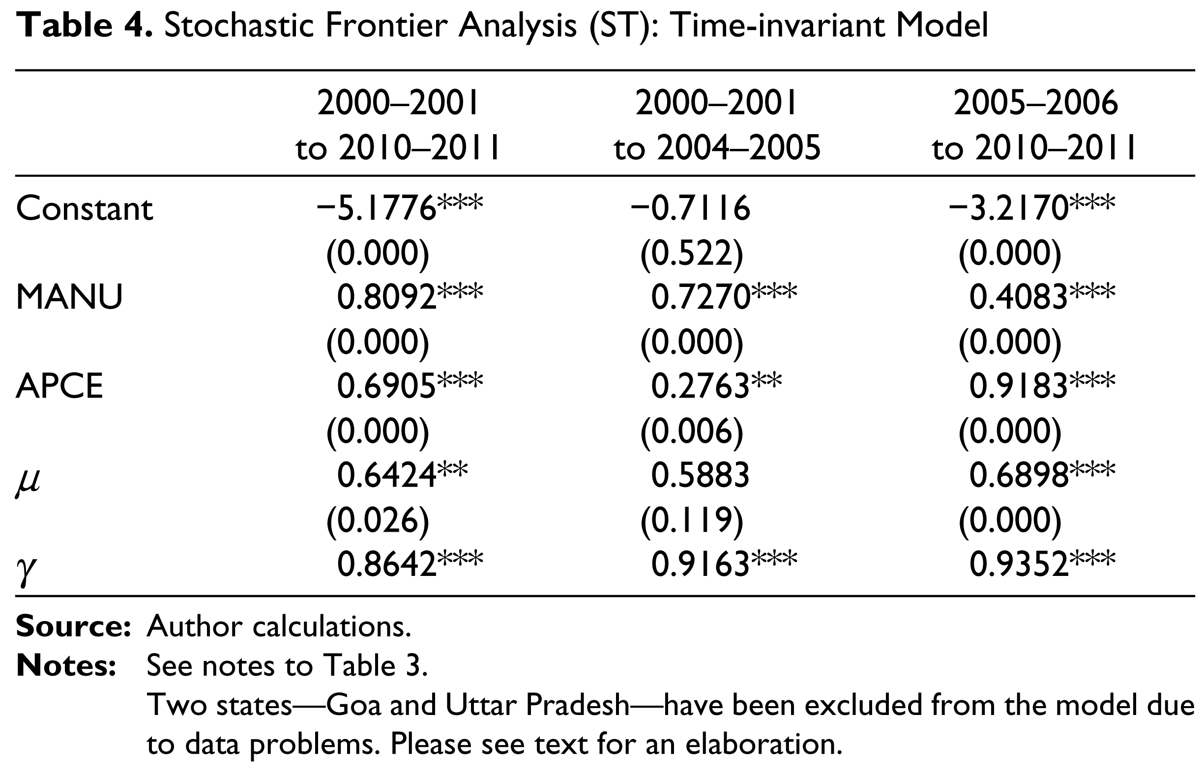
Two states—Goa and Uttar Pradesh—have been excluded from the model due to data problems. Please see text for an elaboration.

State Excise Duty (EX)

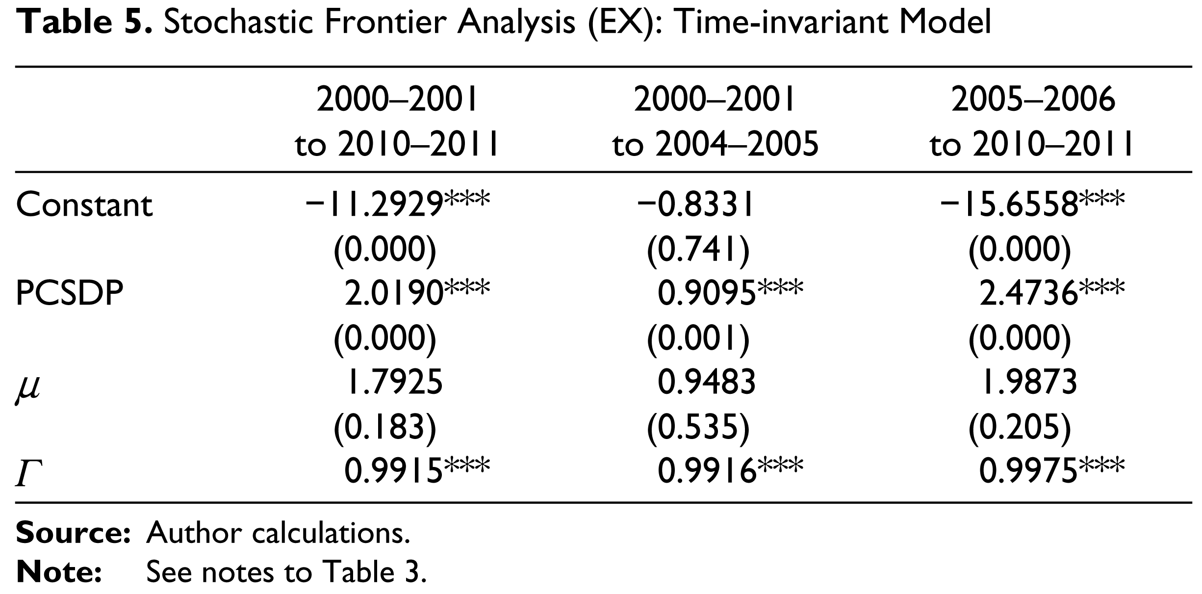
EX is levied by all states and a substantial contribution to this tax comes from the imposition of the levy on the production and consumption of different varieties of alcohol/liquor. As noted by Purohit (2006), ‘the tax is not levied on the production price only. It is sometimes levied on the basis of consumption, especially in those states where there is no production. Hence…this tax [is related] to the consumption of beer or spirit or Indian Made Foreign Liquor’.⁴ Ideally, the base of the tax should be the consumption of different varieties of liquor, data on which is, unfortunately, scarce. The proxy we use to represent the underlying variable of interest is per capita GSDP (PCSDP). The estimated equation is reported in Table 5.

PCSDP appears to be a good proxy of the tax base for EX and is positive and statistically significant in all three time periods. A significant γ statistic with a coefficient close to unity in all three time periods indicates that deviations from the frontier can be largely ascribed to technical inefficiency.

Table 5.

Stochastic Frontier Analysis (EX): Time-invariant Model

	2000–2001 to 2010–2011	2000–2001 to 2004–2005	2005–2006 to 2010–2011
Constant	−11.2929***(0.000)	−0.8331(0.741)	−15.6558***(0.000)
PCSDP	2.0190***(0.000)	0.9095***(0.001)	2.4736***(0.000)
μ	1.7925(0.183)	0.9483(0.535)	1.9873(0.205)
Γ	0.9915***	0.9916***	0.9975***

Source: Author calculations.

Note: See notes to Table 3.

Motor Vehicles Tax (MVT)

MVT combines taxes on vehicles and taxes on goods and passengers. These two taxes have been combined together since the base for both these taxes is, by and large, the same even though in some states these taxes are levied separately. The tax on vehicles is levied at the time of registration of vehicles, on the issuance of permits and certificates of fitness for vehicles and while issuing trade certificates to manufacturers and dealers under the Indian Motor Vehicles Act, 1939. The tax rates vary across states depending on whether the vehicle is being used for private or commercial purposes. The tax is also sometimes based either on the seating capacity of the vehicle or on the registered laden weight, as in the case of two-wheel vehicles. Tax on goods and passengers, on the other hand, is levied on the movement of goods and passengers. It is levied in some states as a percentage of gross revenues from passenger fares and freight of transport companies while in other states, it is levied as a lump sum tax on the basis of seating capacity of the vehicle and length of the routes. The ideal base for this tax is gross revenues of private as well as public transport companies and the fares charged plus the freight chart and/or the volume of passenger traffic and freight transported. Such data are, however, not available for private transport companies. The proxy we use is the sectoral share of GSDP from manufacturing (MANU) and the number of registered motor vehicles in a state (REGVEH). Table 6 reports the results.

Table 6.

Stochastic Frontier Analysis (MVT): Time-invariant Model

	2000–2001 to 2010–2011	2000–2001 to 2004–2005	2005–2006 to 2010–2011
Constant	−10.5901***(0.000)	−7.4219***(0.000)	−7.4069***(0.000)
REGVEH	1.0941***(0.000)	0.9313***(0.000)	0.8761***(0.000)
MANU	0.1230(0.172)	0.0499(0.676)	0.1227(0.504)
μ	0.9878***(0.000)	0.7433**(2.53)	0.8028**(0.019)
γ	0.8196***	0.7021	0.8367***

Source: Author calculations.

Note: See notes to Table 3.

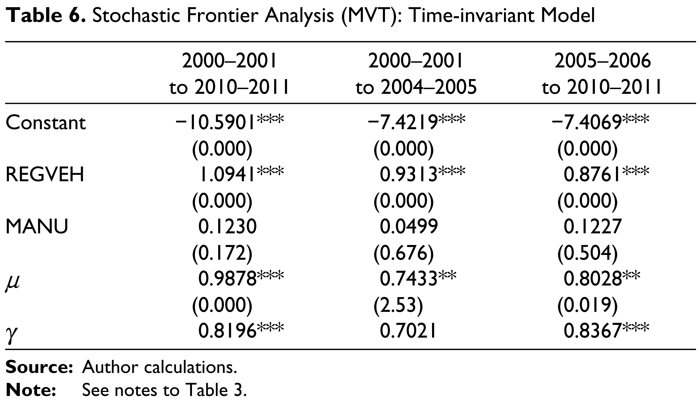
The results for MVT indicates that REGVEH has a positive and significant impact on the tax collections from this revenue head in all three time periods while MANU is significant in none of the three time periods. This could probably be due to the inability of the proxy variable for this tax base to entirely capture the revenues from passenger and freight traffic of transport companies. The γ statistic is significant for the entire time period and in the second sub-period. It is noteworthy that the value of γ is higher in the second sub-period as compared to the entire time-period indicating that inefficiency has increased over time.

Own-Tax Revenue (OTR)

For estimating the equation for OTR, PCSDP acts as a proxy for the level of development of a state. Higher levels of PCSDP translate into a higher demand for public goods and services, and increase the overall ability to pay taxes in a society leading to higher tax compliance and collections (Fox & Gurley, 2005). We initially considered four important factors that possibility affect the revenue raising potential of the states, namely, size of agricultural GSDP, degree of urbanization as reflected by the proportion of urban population to total population of a state, the dependency ratio (understood as the share of population that does not contribute to production; specifically, it is defined as population in the 0–14 years and 60+ year age brackets as a percentage of total population) and per capita GSDP. A proxy for quality of governance is also considered important but such data are not available at the level of states in India. After experimenting with the four factors just mentioned, we finally estimated a parsimonious model for OTR with only two regressors: PCSDP and dependency ratio (DEPRATIO). Table 7 reports the results.

Table 7.

Stochastic Frontier Analysis (OTR): Time-invariant Model

	2000–2001 to 2010–2011	2000–2001 to 2004–2005	2005–2006 to 2010–2011
Constant	0.4391(0.858)	26.7633***(0.000)	−5.8805***(0.003)
PCSDP	1.9212***(0.00)	0.8113***(0.009)	2.1112***(0.000)
DEPRATIO	−1.1736***(0.004)	−5.3218***(0.000)	0.0420(0.899)
μ	1.6388*(0.060)	1.5907**(0.035)	1.7675**(0.020)
γ	0.9944***	0.9939***	0.9981***

Source: Author calculations.

Note: See notes to Table 3.

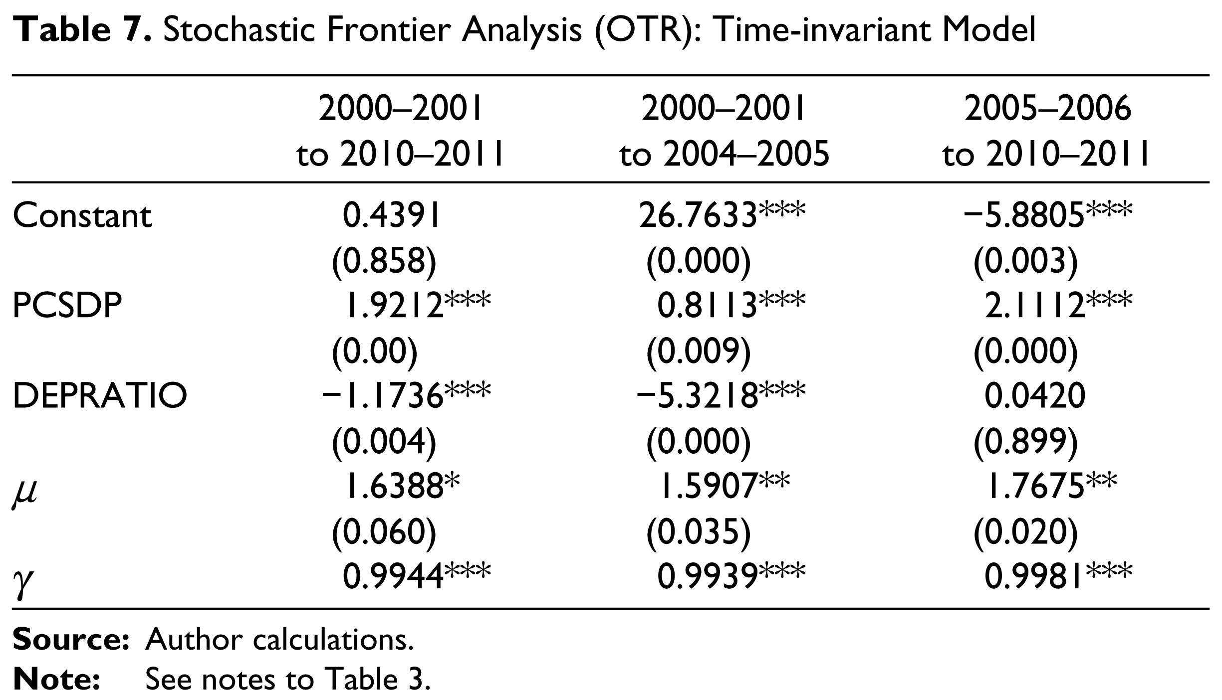
The results show that PCSDP is positive and significant in all the three time periods while DEPRATIO is negative as expected but significant only in the first two time periods. The estimate of γ is consistently high and significant. Its value so close to one indicates that deviations from the frontier are mainly due to technical inefficiency.

Explaining Inefficiency in Tax Collection

Our results for all taxes including OTR have demonstrated the existence of inefficiencies. While it is true that the factors behind the inefficiencies in the collection of all taxes need to be probed further, we confine our attention to OTR alone. We do this for two reasons: one, OTR is a summary measure of the revenue collection performance of the state and an understanding of the macro factors underlying this inefficiency is important; two, the explication of the factors underlying collection of each of the individual taxes would require micro level information which, perhaps, may not be available at a sufficiently disaggregated level.

The literature has pointed towards a few possible reasons for the poor revenue collection performance of states. We discuss some of these and then, wherever appropriate data are available, we estimate an equation to try and explain (in)efficiencies in tax collection.

At the outset it is important to realize that significant parts of a state’s economy remains outside the pale of state-level taxation. The services sector cannot be taxed by states at the moment though this is likely to change with the introduction of the Goods and Services Tax (see below for details). As far as the sales tax (VAT) is concerned, a variety of exemptions are offered by state governments. See Government of Maharashtra (2005) for an illustrative list of commodities which are taxed below the peak rate of 12.5 per cent. Rajaraman (2005) points to the reluctance of Indian states to tax agriculture. Land revenue and agricultural income tax contributed a mere 0.6 per cent of total national (federal plus state governments) tax revenue and just 1.5 per cent of tax revenues collected by the states (Rajaraman, 2005). It is quite clear that significant amount of revenue loss to states has resulted from either their inability or reluctance to tax certain sectors under their domain. However, obtaining state-wise estimates of revenue loss resulting from these factors represents a major challenge. Consequently, while recognizing this as a major drag on the tax performance of states, we have not been able to capture this in the exercise that follows.

The activities of small enterprises, in particular, and the informal sector, in general, lie outside the purview of taxation by state governments. All enterprises having a production of less than ₹1 million are exempt from VAT payable to state governments (Bagchi, Rao & Sen, 2005). This, it has been suggested, creates incentives for such enterprises to remain small (Chatterjee, 2011) and, hence, continue to locate themselves in the informal sector. In an interesting study, Dutta, Kar & Roy (2013) examine the impact of corruption on the size of the informal sector for 20 Indian states for 2004–2005 and find that a higher level of corruption leads to a larger informal sector. However, the authors caution against presuming a causal link between corruption and the informal sector. Form the point of view of the present article, the association between the two is enough to have implications for efficiency in tax collection. Corruption by itself has been blamed for lower tax collections (see below for a discussion) and its effect is further accentuated by providing an impetus to the informal sector which is difficult to tax. In the estimated equation reported below, we proxy the contribution of small enterprises to a state’s production using the percentage of non-farm workers in the unorganized sector in each state (Sakthivel & Joddar, 2006).

The contribution that federal transfers and grants make to the total revenue collection of states has been stated to be a factor in the poor fiscal performance of sub-national governments (Singh & Plekhanov, 2005). There are two possibilities here: one, states may substitute federal transfers for own revenue collection efforts (as measured by OTR); alternatively, it is possible that additional transfers could encourage states to collect more OTR since, in India, most Finance Commission awards have attached some weight to the state’s revenue collection efforts while devising the formulae for federal transfers to states. We will examine the importance of this variable, which has been called Vertical Fiscal Imbalance (VFI) and is defined as the ratio of federal transfers to total revenue account receipts of a state.

Burdening states with expenditure responsibilities has also been suggested to be a factor affecting fiscal performance of sub-national governments (Rodden, 2002). To examine this, we introduce a variable to measure the decentralization of expenditure responsibilities, which is computed as a state’s total expenditure as percentage of expenditure of all levels of government.

Corruption has often been implicated in the poor revenue collection efforts of a state (Cule & Fulton, 2009; Goerke, 2006; Planning Commission, 1999). We have created a measure of corruption based on the data reported by the National Crime Records Bureau (various issues). The data reported refers to persons arrested under the Prevention of Corruption Act and other provisions of the Indian Penal Code. A whole range of data has been collected on ten measures of persons arrested for corruption. Given the plethora of data, we have used factor analysis to group the data into two factors (please see Appendix for details). In addition to the indicator of corruption based on the data of National Crime Records Bureau, we have also experimented with such data reported by Transparency International India (2005).

For the OTR model estimated for entire time period, 2000–2001 to 2010–2011, we obtained estimates of efficiency which range from 1 to 0, with high values indicating better efficiency in OTR collection. Since we have employed a time invariant SFA model, the efficiency values for each state are uniform over the entire time period. Given this uniformity of efficiency values, we select as our data one efficiency value for each of the 17 states we have considered. This gives us the following model:

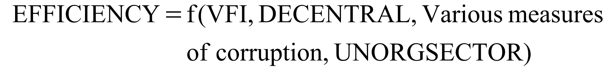
\begin{matrix} E F F I C I E N C Y = f (V F I, D E C E N T R A L, V a r i o u s m e a s u r e s \\ o f c o r r u p t i o n, U N O R G S E C T O R) \end{matrix}

(5)

where,

EFFICIENCY = efficiency in OTR collection

VFI = Vertical Fiscal Imbalance (federal transfers as percent of total revenue account receipts of a state)

DECENTRAL = measure of decentralization (state’s total expenditure as percent of expenditure of all levels of government)

CORRUPT(A)1 = factor 1 of corruption measure A (see Appendix)

CORRUPT(A)2 = factor 2 of corruption measure A (see Appendix)

CORRUPT(B)1 = factor 1 of corruption measure B (see Appendix)

CORRUPT(B)2 = factor 2 of corruption measure B (see Appendix)

UNORGSECTOR = percentage of non-farm workers in the unorganized sector.

In Table 8, we report only some of the equations that we estimated. Specifically, it may be noted that size of unorganized sector and measure of corruption as reported by Transparency International India (2005) did not yield results that were statistically significant. Hence, equations with these variables have not been reported.

There is a possibility that VFI may be endogenously determined since states could behave strategically to be lax about OTR collection in the hope of higher federal transfers; equally likely, higher federal transfers might be directed towards states that perform poorly. Hence, we have estimated the EFFICIENCY equation using OLS as well 2SLS techniques. The estimated equations are given in Table 8.

Focusing on the equations estimated using 2SLS (columns 2 and 4 in Table 8), there is one similarity and two main differences. The similarity is that the variable DECENTRAL is significant and positive in both the equations. Hence, DECENTRAL appears to encourage OTR collection, which suggests that states strive to improve their tax collection in order to meet their expenditure responsibilities. The first difference is with respect to VFI. In column 2, VFI is not statistically significant while, in column 4, it is significant at the 10 per cent level. Hence, as per column 4, there seems to be a complementarity between VFI and efficiency of OTR collections. The second difference between columns 2 and 4 is with respect to the measure of corruption. Even though CORRUPT(A)1 and CORRUPT(B)1 measure the same phenomenon (the correlation between them is 0.8993), the measure in column 2 has a larger coefficient and is significant at 1 per cent level, while the measure in column 4 has a much smaller coefficient and is significant at 5 per cent. Whichever measure of corruption is used, the negative coefficient clearly indicates that, as corruption rises, efficiency in OTR collection goes down. Clearly, reduction of corruption is important for OTR collections.

Table 8.

Explaining Efficiency in OTR Collection

	OLS	2SLS	OLS	2SLS
	(1)	(2)	(3)	(4)
VFI	0.0071***(0.00)	0.0052(0.23)	0.0074***(0.00)	0.0078*(0.08)
DECENTRAL	0.6027***(0.00)	0.6089***(0.00)	0.5240***(0.00)	0.5234***(0.00)
CORRUPT(A)1	−0.0125***(0.01)	−0.0130***(0.00)	–	–
CORRUPT(B)1	–	–	−0.0090*(0.08)	−0.0089**(0.03)
CONSTANT	−0.2085***(0.01)	−0.1370(0.41)	−0.02102** (0.03)	−0.2250 (0.19)
R²	0.8465	0.8270	0.8016	0.8007
Adjusted R²	0.8111	0.7871	0.7558	0.7547
No. of Observations	17	17	17	17
Instruments used in 2SLS estimation		DECENTRAL CORRUPT(A)1CORRUPT(B)1CORRUPT(B)2		DECENTRAL CORRUPT(A)1CORRUPT(B)1CORRUPT(B)2

Source: Author calculations.

Notes: *** = p < 0.01; ** = p < 0.05; * p = < 0.1.

To summarize, the results of Table 8 show that (a) increasing federal transfers (VFI) and decentralization (DECENTRAL) is likely to improve efficiency in OTR collection; (b) reducing corruption will also improve OTR collection.

Estimating Tax Effort

Having estimated SFA models for the various taxes imposed by Indian states, we are now in a position to evaluate their tax effort. We compare the actual tax revenues collected with the estimated tax potential for each of the taxes studied. The estimated tax potential is nothing but the predicted values of the taxes obtained from the SFA equations. The computed tax effort or the extent of tax potential used indicates the efficiency with which states are utilizing their potential and the average for all 17 states may be interpreted as ‘industry efficiency’. Our primary interest in this section is not only to estimate tax effort for the various taxes but, more importantly, to find out if tax effort has improved or deteriorated over time. Specifically, we wish to compare tax effort in the first sub-period 2000–2001 to 2004–2005 with that in the second sub-period 2005–1006 to 2010–2011.

Table 9 gives estimates of tax effort for STAMPS.

Only three states show tax effort above the 50 per cent mark in the second sub-period: Bihar, Punjab and Chhattisgarh. All the other states languish substantially below the half-way mark. The average for both segments of the time period under consideration is around 40 per cent. The positive development that can be discerned from Table 9 is that tax effort performance has shown improvement in the second sub-period with only six of the 17 states showing a negative entry in the last column of the table.

The results of Table 9 clearly suggest that states have been very lax in exploiting this source of tax and there remains much unexploited tax potential which can be tapped. One reason that can possibly explain this slack in performance across states is that Stamp Duty is levied at different rates across states, which is usually very high and the additional imposition of registration fees results in high marginal rates of tax. This has resulted in large-scale evasion of the tax by undervaluing the value of the property and this has been further aggravated by the presence of unorganized property market for urban immovable property. The development of an organized market for urban immovable property can help overcome this problem but would require a mechanism which can differentiate the various types of property and set objective benchmarks by taking into consideration value of land, cost of building, etc. (Rao, 2002; Rao & Rao, 2005).

Table 9.

Tax Effort: Stamp Duty and Registration Fees (STAMPS) (%)

	2000–2001 to 2004–2005	2005–2006 to 2010–2011	Change
Andhra Pradesh	25.56	30.71	5.15
Bihar	81.77	53.92	−27.85
Chhattisgarh	43.17	54.02	10.85
Goa	37.67	43.47	5.8
Gujarat	36.61	34.04	−2.57
Haryana	51.44	48.69	−2.75
Jharkhand	31.89	28.86	−3.03
Karnataka	32.71	33.71	1
Kerala	23.70	35.15	11.45
Madhya Pradesh	38.37	49.04	10.67
Maharashtra	29.28	34.08	4.8
Orissa	14.02	21.77	7.75
Punjab	84.45	86.68	2.23
Rajasthan	27.76	33.01	5.25
Tamil Nadu	29.75	26.18	−3.57
Uttar Pradesh	46.90	48.32	1.42
West Bengal	28.37	27.31	−1.06
Average	39.02	40.53	1.51

Source: Author calculations.

Note: Change is computed as tax effort in the period 2005–2006 to 2010–2011 minus tax effort in the period 2000–2001 to 2004–2005. A positive value indicates improvement while a negative sign indicates deterioration.

Table 10 reports tax effort for ST.

Table 10.

Tax Effort: State Sales Tax (ST) (%)

	2000–2001 to 2004–2005	2005–2006 to 2010–2011	Change
Andhra Pradesh	158.23	95.22	−63.01
Bihar	103.84	50.36	−53.48
Chhattisgarh	30.45	29.94	−0.51
Goa*	–	–	–
Gujarat	57.06	46.54	−10.52
Haryana	52.99	33.62	−19.37
Jharkhand	30.05	26.89	−3.16
Karnataka	112.27	65.31	−46.96
Kerala	124.45	60.16	−64.29
Madhya Pradesh	79.85	55.45	−24.4
Maharashtra	87.34	67.44	−19.9
Orissa	73.08	46.81	−26.27
Punjab	55.73	29.09	−26.64
Rajasthan	89.35	53.93	−35.42
Tamil Nadu	121.16	70.10	−51.06
Uttar Pradesh*	–	–	–
West Bengal	86.21	53.20	−33.01
Average	84.14	52.27	−31.87

Source: Author calculations.

Notes: Please see note to Table 9.

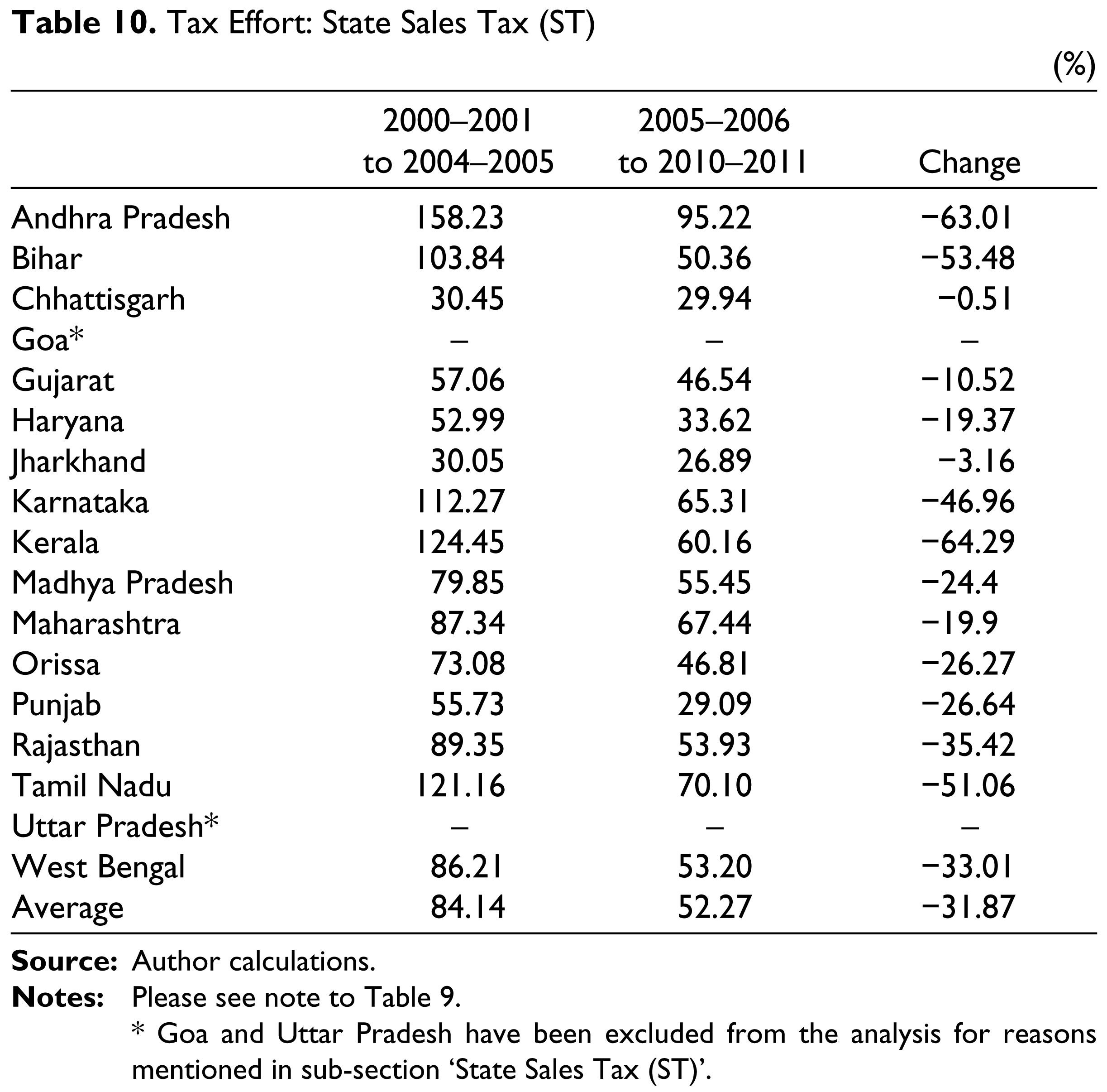
* Goa and Uttar Pradesh have been excluded from the analysis for reasons mentioned in sub-section ‘State Sales Tax (ST)’.

The performance is much better in the case of ST as compared to STAMPS but, even here, there is evident slippage in performance in the second half of the time period under consideration with the average rate falling from 84 per cent to 52 per cent. What is true for the average is true for each and every state with all states showing deterioration in performance. The worst deterioration is seen in the case of Kerala with a fall of 65 percentage points and Andhra Pradesh with a fall of 63 percentage points. It is important to note that the second time period 2005–2006 to 2010–2011 covers the period when VAT was implemented across all states, indicating thereby that revenue performance has shown a decline under the VAT regime. This decline can be attributed to reasons such as differing VAT across states with different thresholds for registration of VAT dealers, simplified tax regime in some states with no input crediting for dealers below the VAT threshold, exclusion of certain goods including basic necessities, petroleum, oil and lubricants from VAT and limits on VAT credit for inputs and capital goods (Das-Gupta, 2012). The audit conducted by the Comptroller and Auditor General (CAG) of India (2010) on VAT performance covering 23 states for the period 2005–2006 to 2008–2009 also highlighted several ills plaguing VAT implementation, such as, deficiencies in VAT acts and rules in many states, large backlog of pending assessments under predecessor taxes (sales tax), incomplete automation and limited electronic return filing of the tax, ineffective procedures for verification of input tax credit (ITC) claims and detecting fake ITC claims and problems in dealer registration procedures, among others. The audit found widespread tax evasion and avoidance through under-declaration of sales and incorrect or fake ITC claims by about 50 per cent of VAT dealers, grant of incorrect VAT exemptions and non-remittance of VAT collected from customers by some exempt dealers. All these factors highlight the problems in the administration of VAT and explain the substantial decline seen in revenues under this tax during the period 2005–2006 to 2010–2011. Table 11 reports results of tax effort for EX.

Table 11.

Tax Effort: State Excise Tax (EX) (%)

	2000–2001 to 2004–2005	2005–2006 to 2010–2011	Change
Andhra Pradesh	40.01	14.58	−25.43
Bihar	17.13	47.19	30.06
Chhattisgarh	9.66	6.02	−3.64
Goa	0.39	0.02	−0.37
Gujarat	0.84	0.07	−0.77
Haryana	14.54	1.83	−12.71
Jharkhand	5.38	3.24	−2.14
Karnataka	45.54	14.55	−30.99
Kerala	12.20	2.18	−10.02
Madhya Pradesh	32.55	27.49	−5.06
Maharashtra	33.24	4.82	−28.42
Orissa	7.42	4.61	−2.81
Punjab	23.65	15.60	−8.05
Rajasthan	33.63	14.36	−19.27
Tamil Nadu	39.41	8.79	−30.62
Uttar Pradesh	94.32	93.27	−1.05
West Bengal	14.30	5.71	−8.59
Average	24.95	15.55	−9.4

Source: Author calculations.

Note: Please see note to Table 9.

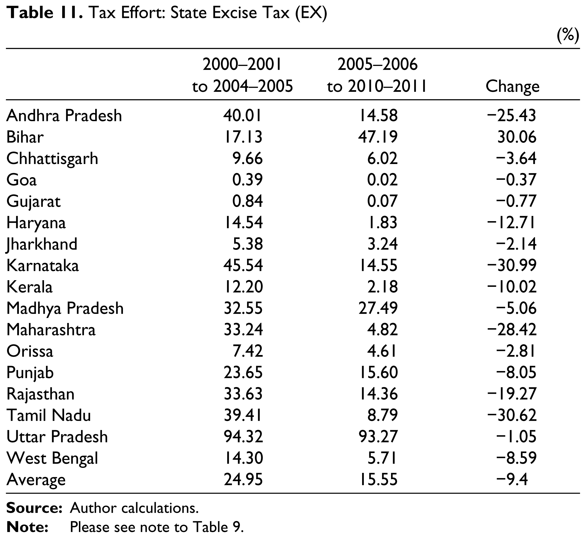
As in the case of state sales tax, the tax effort for excise duty has declined by almost 0 percentage points from 24.95 per cent in 2000–2001 to 2004–2005 to 15.55 per cent in 2005–2006 to 2010–2011. This has been reflected in a decline in effort in all the 17 states except Bihar whose tax effort more than doubled from 17.13 per cent in 2000–2001 to 2004–2005 to 47.19 per cent in 2005–2006 to 2010–2011. Uttar Pradesh is the best performing state which has shown a tax effort of more than 90 per cent. More than half of the states (nine of 17) have seen substantial decline in tax effort for EX. These states are Andhra Pradesh, Haryana, Karnataka, Kerala, Maharashtra Punjab, Rajasthan, Tamil Nadu and West Bengal. The inordinately low numbers for Gujarat may be attributed to the policy of prohibition of alcohol sales in the state which reduces the revenue collected under this tax. The illicit brewing and consumption of country liquor and the large-scale evasion of tax in the case of IMFL has led to a substantial loss in revenue. For instance, an estimate of the evasion of the tax can be made from the findings of the Karnataka Tax Reforms Committee which noted the evasion to be three times the actual revenue collected from the tax (Rao & Rao, 2005).

Table 12 reports results of tax effort for MVT.

Table 12.

Tax Effort: Motor Vehicle Tax (MVT) (%)

	2000–2001 to 2004–2005	2005–2006 to 2010–2011	Change
Andhra Pradesh	46.19	42.69	−3.5
Bihar	89.28	117.03	27.75
Chhattisgarh	68.46	67.97	−0.49
Goa	40.86	60.26	19.4
Gujarat	32.25	24.35	−7.9
Haryana	65.81	31.79	−34.02
Jharkhand	27.14	33.54	6.4
Karnataka	74.91	71.17	−3.74
Kerala	46.02	38.27	−7.75
Madhya Pradesh	52.64	61.26	8.62
Maharashtra	39.05	34.91	−4.14
Orissa	91.65	83.23	−8.42
Punjab	26.27	20.57	−5.7
Rajasthan	51.28	41.84	−9.44
Tamil Nadu	40.12	41.05	0.93
Uttar Pradesh	27.31	25.19	−2.12
West Bengal	36.41	36.39	−0.02
Average	50.33	48.91	−1.42

Source: Author calculations.

Note: Please see note to Table 9.

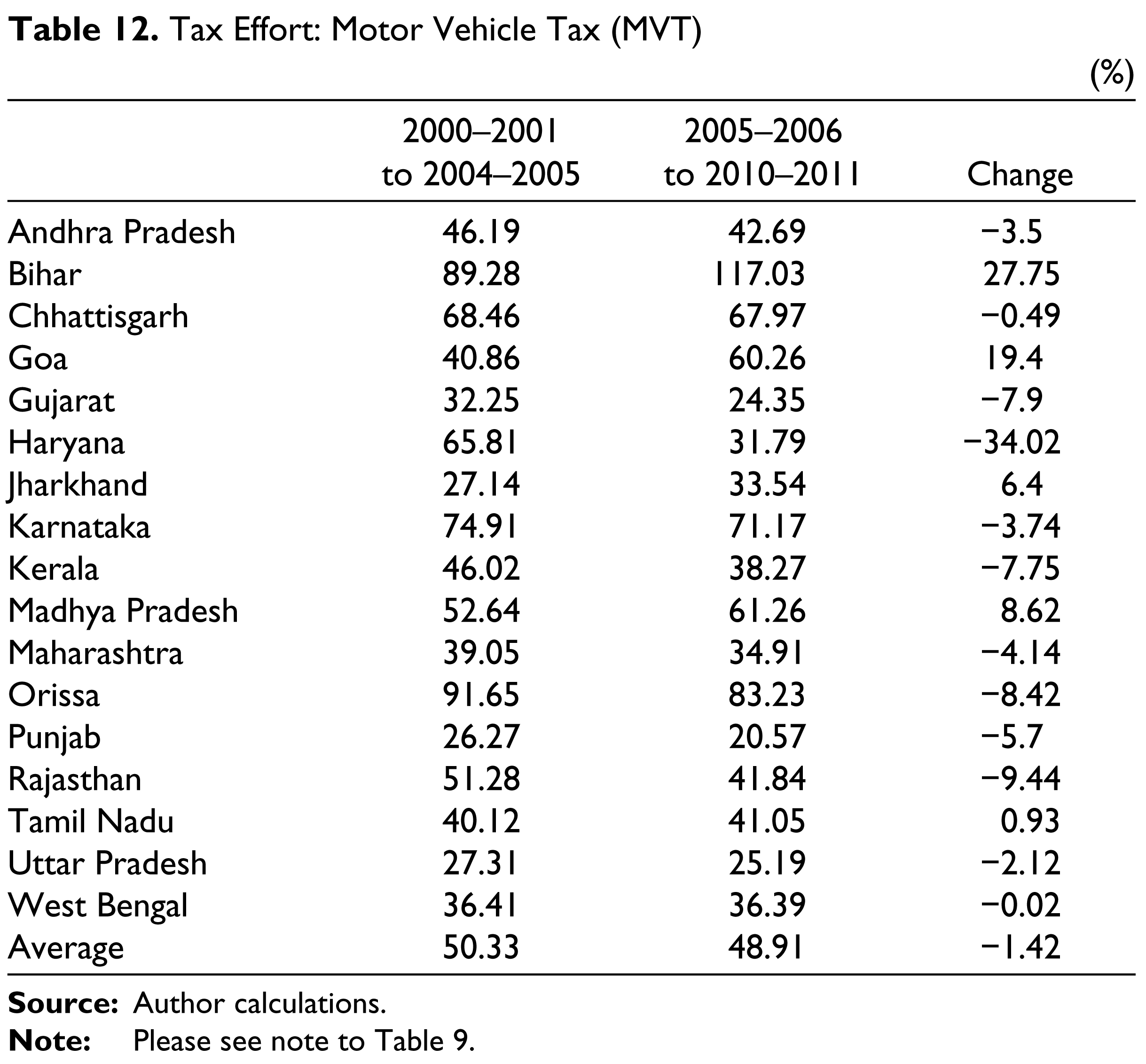
The average tax effort for MVT has declined marginally from 50 per cent in 2000–2001 to 2004–2005 to 48.91 per cent in 2005–2006 to 2010–2011. Of the 17 states, only five have shown an improvement in the second sub-period. Bihar, Chhattisgarh, Karnataka and Orissa have exploited more than 60 per cent of the tax potential while Uttar Pradesh and Punjab have exploited less than 30 per cent of the potential under this tax in both periods. Rao and Rao (2005) point out that for administrative convenience, many states have merged the tax on passengers and goods with the tax on vehicles. Also, the tax on private non-commercial vehicles has been converted into a lifetime tax by adding up ten years’ tax or by adopting a similar formula. Hence, the reform that has been suggested is to separate the tax on vehicles from the tax on passengers and goods and that the tax on passengers and goods should be a part of state VAT instead of a separate tax. Finally, Table 13 reports tax effort for OTR.

Table 13.

Tax Effort: Own-Tax Revenues (OTR) (%)

	2000–2001 to 2004–2005	2005–2006 to 2010–2011	Change
Andhra Pradesh	21.22	20.51	−0.71
Bihar	34.44	56.28	21.84
Chhattisgarh	7.98	7.87	−0.11
Goa	0.18	0.12	−0.06
Gujarat	14.92	8.10	−6.82
Haryana	10.42	3.68	−6.74
Jharkhand	8.27	8.20	−0.07
Karnataka	17.46	16.36	−1.1
Kerala	7.38	6.27	−1.11
Madhya Pradesh	30.33	30.89	0.56
Maharashtra	34.14	15.06	−19.08
Orissa	8.44	10.87	2.43
Punjab	7.68	4.77	−2.91
Rajasthan	31.71	20.60	−11.11
Tamil Nadu	14.22	13.26	−0.96
Uttar Pradesh	93.32	96.28	2.96
West Bengal	14.37	15.22	0.85
Average	20.97	19.67	−1.3

Source: Author calculations.

Note: Please see note to Table 9.

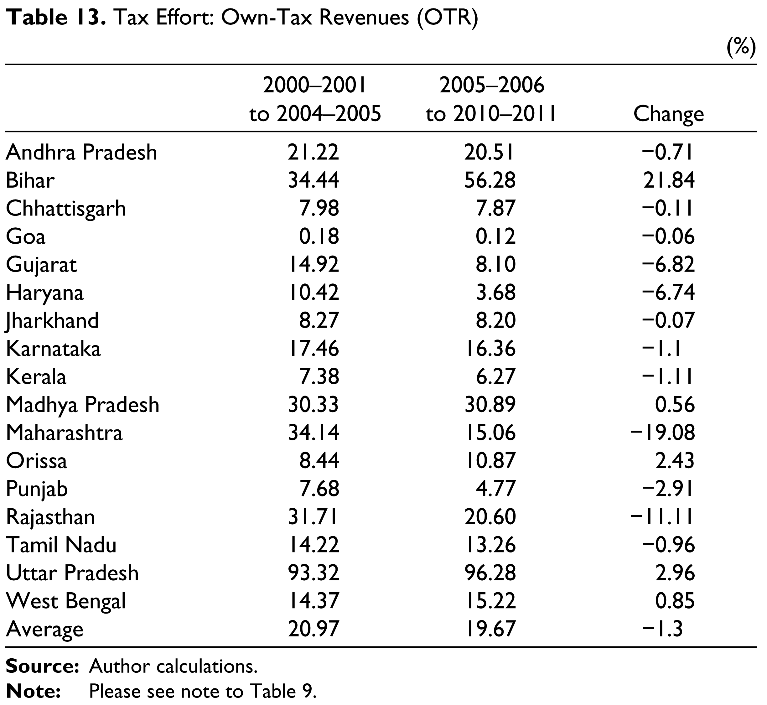
Tax effort for the totality of all taxes collected by the state, namely, own-tax revenues, is a significant cause for concern since, on average, states have exploited only about 20 per cent of the overall potential in the two sub-periods. Only five states—Andhra Pradesh, Bihar, Madhya Pradesh, Rajasthan and Uttar Pradesh—show above average performance. Comparing the two sub-periods, most states exhibit a change in performance that is negative or only marginally positive. Only Bihar shows an improvement of 21.84 percentage points.

The main finding to emerge from Table 13 is that states have not exploited their tax bases adequately and this is the reason for their excessive dependence on transfers from the federal government. While the performance has been very disappointing, the silver lining, if any, is that the low utilization of the tax potential suggests that there is great room available for improvement. This improvement in tax effort will be able to afford states a substantial increase in the fiscal space available to them. Quite clearly strengthening the tax administration and strict enforcement would help increase compliance and revenues of the states (Rao, 2002).

Conclusion

This article has explored the potential of 17 Indian states to generate fiscal space by studying the tax effort of these states. Using SFA, we have studied the revenue raising potential for four major taxes at the state level, namely, stamp duty and registration fees, state sales tax, state excise duty and motor vehicles tax as well as for own tax revenue. The choice of regressors, which proxied the tax base for each of these taxes, was determined by theory and by availability of data. The results indicate that for each of the taxes considered in the article, technical inefficiency (represented by the γ coefficient being close to unity for all the estimated equations) emerged as the primary reason for states not being able to generate revenues close to their potential.

The tax effort analysis highlighted the substantial decline over time in the average tax effort for two major state level taxes, state sales tax and state excise duty and a marginal decline in the tax effort for motor vehicles tax and own tax revenues. Tax effort for stamp duty and registration fee has shown an increase over the two periods. The tax effort analysis also points to the large budgetary room that states have in raising additional revenues from existing taxes. Analyzing the determinants for efficiency in tax collections we have found complementarity between vertical fiscal transfers received by states and their OTR revenues as also evidence that the decentralization of government expenditure helps improve efficiency of OTR collections. Inclusion of a measure of corruption highlights the inverse relationship between corruption and efficiency in OTR collections. Hence, a reduction in corruption is vital for improvements in OTR collections.

Efforts at enhancing internal fiscal capacity at the state level should focus on improving the ratio of OTR to GDP. The Fourteenth Finance Commission expects this ratio to reach an average level of about 8.5 per cent over the time period of its award, 2015–2016 to 2019–2020 (Government of India, 2015). The OTR–GSDP ratio can be improved by improving revenue buoyancy, better tax administration and plugging revenue leakages and thus reducing inefficiency. Given that many states have been lagging behind in their OTR performances, a major boost along these lines has become imperative.

Much hope has been placed on the introduction of the Goods and Services Tax (GST) for increasing revenue collection by the federal and state governments. It is seen as the next most important tax reform after the introduction of VAT in 2005 (Poddar & Ahmad, 2009). Two important factors have been adduced in justifying the significance of the GST: one, the traditional distinction between goods and services has become blurred in recent years and, hence, the sales tax, which is a tax on goods sold, has lost its bite; two, the exclusion of services from the taxing powers of state has had a negative effect on the buoyancy of state taxes. As per the recommendation of the Kelkar Committee (Government of India, 2004), both goods and services would be subject to concurrent taxation by the centre and the states. The state taxes and levies that will be subsumed under GST include VAT/sales tax, entertainment tax, luxury tax, taxes on lottery, betting and gambling, state cess and surcharges relating to the supply of goods and services and entry tax not in lieu of octroi (Government of India, 2015). The two most significant benefits of the GST are expected to be revenue generation apart from removal of distortions due to taxation and the creation of common market in India (Government of India, 2015; Rao, 2011). Apart from expanding the bases available for state taxation, it is felt that introduction of GST will change the incentive structure especially with respect to incentives to evade taxes. In view of the expected lower rate of tax and elimination of cascading effects, tax payers may be encouraged to pay their taxes to a greater extent than earlier.

If the touted benefits of the GST are, indeed, realized, the problems with inefficiency in tax collections that have been pointed out by this article may well cease to be relevant. However, just as problems with respect to implementation of VAT still persist 10 years after its introduction, the transition to a GST regime may well take considerable time and effort. In this context, Das-Gupta (2012) has sounded a note of caution bearing in mind the poor preparedness of tax administration in various states. Rao (2011) has also reminded us that a one-size-fits-all approach towards all states may well run up against state-specific problems. More importantly, doubts have been raised about the exact scale of revenue generation by the state. The Fourteenth Finance Commission (Government of India, 2015, p. 176) has stated ‘…we are unable to estimate revenue implications and quantify the amount of compensation in case of revenue loss to the states due to the introduction of GST’. Hence, given this uncertainty and the apprehensions of the states, the Commission has recommended that states should receive revenue compensation for five years as compared to the three years compensation that was provided to the states following the introduction of the VAT. Bearing in mind all these uncertainties surrounding the introduction and implementation of the GST, it is our belief that the results obtained in this paper are likely to remain relevant even during the post-GST regime.

Footnotes

Acknowledgements

The authors would like to thank an anonymous referee for making several important suggestions for improving the paper. Of course, the authors remain responsible for any errors that remain in the article.

Notes

Prevention of Corruption

The following data are reported by the National Crime Records Bureau (various issues):

Persons Reported for Regular Departmental Action

Persons Reported for Suitable Action

Persons Punished Departmentally

Dismissed from Service

Removed from Service

Awarded Other Major Punishment

Awarded Minor Punishment

Gazetted or Equal Status Officers in Public Sector Undertaking Involved

Group ‘A’ Officers

Group ‘B’ Officers

Non-Gazetted or Equal Status Officers in Public Undertaking Involved

Private Persons Involved

The absolute numbers of the items listed above have been transformed in two ways: (a) each item is expressed as share of each state out of the total for all states; (b) each item is expressed as a rate per million of population for each state.

Given the large number of heads under which data have been reported, we first aggregated the items under list item three above and those under list item four. After that, factor analysis was employed to create two factors:

Factor 1: Aggregating heads 4, 5 and 6. This translates into measures which we call CORRUPT(A)1 (computed as a share of each state) and CORRUPT(B)1 (computed as rate per million population)

Factor 2: Aggregating heads 1, 2 and 3. This translates into measures which we call CORRUPT(A)2 (computed as a share of each state) and CORRUPT(B)2 (computed as rate per million population).

Even though we have two ways of creating corruption factors, there is high correlation between CORRUPT(A)1 and CORRUPT(B)1 (0.8993) and between CORRUPT(A)2 and CORRUPT(B)2 (0.8725).

References

Aigner

D.J.

, Lovell

C.A.K.

, & Schmidt

(1977). Formulation and estimation of stochastic frontier production models. Journal of Econometrics, 6(1), 21–37.

Aizenman

, & Jinjarak

(2010). De facto fiscal space and fiscal stimulus: Definition and assessment. Working Paper 16539, NBER Working Paper Series.

Alfirman

(2003). Estimating stochastic frontier tax potential: Can Indonesian local governments increase tax revenues under decentralization? Center for Economic Analysis, Department of Economics, University of Colorado, Boulder, Working Paper No. 03-19, November 2003. Retrieved 11 May 2015 , from http://dirwww.colorado.edu/Economics/papers/WPs-03/wp03-19/wp03-19.pdf

Bagchi

, Rao

R.K.

, & Sen

(2005). Tax breaks for the small scale sector: An appraisal. NIPFP Working Paper 6, National Institute of Public Finance and Fiscal Policy, New Delhi. Retrieved 11 May 2015 , from http://www.nipfp.org.in/media/medialibrary/2013/04/wp06_nipfp_tr_042.pdf

Battese

G.E.

, & Coelli

T.J.

(1988). Prediction of firm level technical efficiencies with a generalized frontier production function and panel data. Journal of Econometrics, 38(3), 387–399.

Battese

G.E.

, & Corra

G.S.

(1977). Estimation of a production frontier model: With application to the pastoral zone of Eastern Australia. Australian Journal of Agricultural Economics, 21(3), 169–179.

Chatterjee

(2011). Resource allocation and efficiency in developing countries. A dissertation submitted for the degree of Doctor in Philosophy in Economics at the University of California, Berkeley. Retrieved 11 May 2015 , from http://digitalassets.lib.berkeley.edu/etd/ucb/text/Chatterjee_berkeley_0028E_12118.pdf

Coelli

T.J.

, Rao

D.S.P.

, O’Donell

C.J.

, & Battese

G.E.

(2005). An introduction to efficiency and productivity analysis (2nd ed.). New York: Springer.

Comptroller and Auditor General (CAG) of India. (2010). Implementation of value added tax in India: Lessons for transition to goods and services tax—A study report. Retrieved 11 May 2015 , from http://www.saiindia.gov.in/english/home/Our_Products/Other_Reports/Study_Reports/SRA-value-added-tax.pdf

10.

Coondoo

, Majumdar

, Mukherjee

, & Neogi

(2001). Relative tax performance: Analysis for selected states in India. Economic and Political Weekly, 36(40), 3869–3871.

11.

Çule

, & Fulton

(2009). Business culture and tax evasion: Why corruption and the unofficial economy can persist. Journal of Economic Behavior & Organization, 72(3), 811–822.

12.

Das-Gupta

(2012). An assessment of the revenue impact of state-level VAT in India. Economic and Political Weekly, 67(10), 55–64.

13.

Davoodi

H.R.

, & Grigorian

D.A.

(2007). Tax potential vs. tax effort: A cross-country analysis of Armenia’s stubbornly low tax collection, International Monetary Fund Working Paper, WP/07/106, May 2007.

14.

Dutta

, Kar

, & Roy

(2013). Corruption and persistent informality: An empirical investigation for Indian states. International Review of Economics and Finance, 27(C), 357–373.

15.

Fenochietto

, & Pessino

(2013). Understanding countries’ tax effort, International Monetary Fund Working Paper, WP/13/244, November 2013.

16.

Fox

W.F.

, & Gurley

(2005). An exploration of tax patterns around the world. Tax Notes International: Special Reports, 37(9), 793–807.

17.

Garg

, Goyal

, & Pal

(2014). Why tax effort falls short of capacity in Indian states: A stochastic frontier approach. Indira Gandhi Institute of Development Research Working Paper, WP-2014-032, August 2014.

18.

Goerke

(2006). Bureaucratic corruption and profit tax evasion. CESifo Working papers, No. 1666.

19.

Government of India. (2004). Report of the task force on implementation of the Fiscal Responsibility and Budget Management Act. Ministry of Finance, Government of India, New Delhi. Retrieved 11 May 2015 , from http://finmin.nic.in/reports/FRBM_report.pdf

20.

Government of India. (2015). Report of the Fourteenth Finance Commission, Finance Commission of India, Government of India, New Delhi. Retrieved 11 May 2015 , from http://finmin.nic.in/14fincomm/14thFinanceCommission.htm

21.

Government of Maharashtra. (2005). Schedule A, Department of Sales Tax, Government of Maharashtra. Retrieved 11 May 2015 , from http://mahavat.gov.in/Mahavat/MyFold/KNOWLEDGE%20CENTER/RATE%20SCHEDULE/KNOW_RATESCHEDULE/S%20C%20H%20E%20D%20U%20L%20E.pdf

22.

Heller

P.S.

(2005a). Back to basics—Fiscal space. What it is and how to get it. Finance and Development, 42(2).

23.

Heller

P.S.

(2005b). Understanding fiscal space, IMF Working Paper, PDP/05/4, International Monetary Fund.

24.

Mikesell

(2007). Changing fiscal capacity and tax effort in a era of devolving government, 1981–2003. Publius: The Journal of Federalism–, 37(4), 532–550.

25.

Mohan

, & Shyjan

(2009). Tax devolution and grant distribution to states in India: Analysis and roadmap for alternatives. Centre for Development Studies working Paper number 419. Retrieved 26 April 2015 , from http://www.esocialsciences.org/Download/repecDownload.aspx?fname=Document11522010460.4993097.pdf&fcategory=Articles&AId=2421&fref=repec

26.

National Crime Records Bureau. (various issues). Crime in India: Statistics. Ministry of Home Affairs, Government of India, New Delhi.

27.

Oommen

M.A.

(1987). Relative tax effort of states. Economic and Political Weekly, 22(11), 466–470.

28.

Ostry

J.D.

, Ghosh

A.R.

, Kim

I., & Qureshi

M.S.

(2010). Fiscal space, IMF staff position note, SPN/10/11. International Monetary Fund.

29.

Pitt

M.M.

, & Lee

(1981). The measurement and sources of technical inefficiency in the Indonesian weaving industry. Journal of Development Economics, 9(1), 43–64.

30.

Planning Commission. (1999). Medium-term fiscal reforms strategy for states. Planning Commission of India Draft Discussion Paper, Planning Commission of India, New Delhi. Retrieved 10 May 2015 , from http://planningcommission.nic.in/reports/articles/ncsxna/index.php?repts=fiscal.htm#10b

31.

Planning Commission. (2012). Report of the working group on state’s financial resources for the Twelfth Five Year Plan (2012–2017). Planning Commission of India, New Delhi. Retrieved 11 May 2015 , from http://planningcommission.gov.in/aboutus/committee/wrkgrp12/wg_state_finan0106.pdf

32.

Poddar

, & Ahmad

(2009). GST reforms and intergovernmental considerations in India. Working Paper No. 1/2009-DEA, Ministry of Finance, Government of India. Retrieved 11 May 2015 , from http://finmin.nic.in/workingpaper/gst%20reforms%20and%20intergovernmental%20considerations%20in%20india.pdf

33.

Purohit

M.C.

(2006). Tax efforts and taxable capacity of central and state governments. Economic and Political Weekly, 61(8), 747–754.

34.

Rajaraman

(2005). Taxing agriculture in a developing country: A possible approach. In Alm

J.R.

, Martinez-Vazquez

& Wallace

(Eds), Taxing the hard-to-tax: Lessons from theory and practice (Contributions to Economic Analysis, Volume 268) (pp. 245–268). Bingley, UK: Emerald Group Publishing Limited.

35.

Rao

M.G.

(2000). Fiscal decentralization in Indian federalism. Institute for Social and Economic Change, Bangalore. Retrieved 11 May 2015 , from https://www.imf.org/external/pubs/ft/seminar/2000/fiscal/rao.pdf

36.

Rao

M.G.

(2002). State finances in India: A critical review. Institute for Social and Economic Change Working Paper, No. 113, Bangalore.

37.

Rao

M.G.

(2005). Changing contours in federal fiscal arrangements in India. In Bagchi

(Ed.), Readings in public finance (pp. 437–464). New Delhi: Oxford University Press.

38.

Rao

M.G.

(2011). Goods and services tax: A gorilla, chimpanzee or a genus like ‘primates’? Economic and Political Weekly, XLVI(7), 43–48.

39.

Rao

M.G.

, & Rao

R.K.

(2005). Trends and issues in tax policy and reform in India. National Institute of Public Finance and Policy Tax Research Unit Working Paper, No. 1, October 2005.

40.

Reddy

K.N.

(1975). Inter-state tax effort. Economic and Political Weekly, 10(50), 1916–1924.

41.

Reserve Bank of India. (2010). Handbook of statistics on state government finances. July 2010, Reserve Bank of India, Mumbai. Retrieved 11 May 2015 , from https://rbi.org.in/scripts/OccasionalPublications.aspx?head=Handbook%20of%20Statistics%20on%20State%20Government%20Finances%20-%202010

42.

Reserve Bank of India. (2013). State finances: A study of state budgets of 2012–13. Mumbai: Reserve Bank of India.

43.

Rodden

(2002). The dilemma of fiscal federalism: Grants and fiscal performance around the world. American Journal of Political Science, 46(3), 670–687.

44.

Roy

, Heuty

, & Letouzé

(2007). Fiscal space for what? Analytical issues from a human development perspective. Paper for the G-20 Workshop on Fiscal Policy—Istanbul, 30 June 30–2 July 2007, UNDP. Retrieved 11 May 2015 , from http://www.undp.org/content/dam/aplaws/publication/en/publications/poverty-reduction/poverty-website/fiscal-space-for-what/FiscalSpaceforWhat.pdf

45.

Sakthivel

, & Joddar

(2006). Unorganised sector workforce in India: Trends, patterns and social security coverage. Economic and Political Weekly, 41(21), 2107–2114.

46.

Schik

(2009). Budgeting for fiscal space. OECD Journal on Budgeting, 2009(2): 1–18. Retrieved 11 May 2015 , from http://www.oecd.org/gov/budgeting/45361746.pdf

47.

Sen

(1997). Relative tax effort by Indian states, National Institute of Public Finance and Policy Working Paper No. 5.

48.

Singh

, & Plekhanov

(2005). How should sub-national government borrowing be regulated? Some cross-country empirical evidence. International Monetary Fund Working Paper, WP/05/54, March 2005.

49.

Sobarzo

(2004). Tax effort and tax potential of State governments in Mexico: A representative tax system. The Helen Kellogg Institute for International Studies Working Paper No. 315, October 2004. Retrieved 11 May 2015 , from https://kellogg.nd.edu/publications/workingpapers/WPS/315.pdf

50.

Stotsky

J.G.

, & Woldemariam

(1997). Tax effort in sub-Saharan Africa, International Monetary Fund Working Paper, WP/97/107, September 1997.

51.

Tran

T.B.

, Grafton

R.Q.

, & Kompas

(2008). Firm efficiency in a transitional economy: Evidence from Vietnam. Asian Economic Journal, 22(1), 47–66.

52.

Transparency International. (2005). India corruption study 2005. New Delhi: Transparency International India, Lajpat Bhawan, Lajpat Nagar IV.