India’s Balance of Payments,Growth and Fiscal Policy

Abstract

Following a dream run during 2003–2004 to 2010–2011, when India’s annual growth rate averaged close to 9 per cent in the midst of remarkable balance of payments (BOP) stability (except for the year 2008–2009), India has slumped into a recession accompanied by severe BOP difficulties and high rates of consumer price inflation. The Government of India (GoI) has responded to it by cutting down subsidies and hiking indirect tax rates. This article develops a simple Keynesian model to assess the policies noted above. It argues that the policies adopted so far by the GoI are likely to aggravate the problems of recession, BOP difficulties and inflation. It recommends hikes in personal income tax rates with a suitable expenditure policy to get out of the present macroeconomic instability.

JEL Classification: E12, E32, F41

Keywords

India growth net capital inflow Stagflation Indirect tax

Introduction

After a period of remarkably high growth unprecedented in India’s economic history in an environment of stable and favourable balance of payments (BOP) situation, India has entered into a phase of recession accompanied by a highly uncertain and adverse BOP situation and high rates of consumer price inflation. However, as we find from Table A1, India’s growth rate plummeted since 2011–2012. It dropped from 8.4 per cent in 2010–2011 to 6.5 per cent in 2011–2012 and further to 5 per cent and 4.5 per cent in 2012–2013 and 2013–2014, respectively. We also find from Table A2 that there is a strong correlation between the slide in India’s growth rate and the BOP difficulties. Table A2 shows that in 2008–2009, when the growth rate dipped, the exchange rate rose steadily from ₹40.0224 in April 2008 to ₹51.2887 in March 2009. Similarly, during recession years 2011–2012 and 2012–2013, the exchange rate increased unwaveringly from ₹44.4174 in July 2011 to 52.6769 in December 2011 and to ₹51.3992 in January 2012, and again from ₹51.8029 in April 2012 to ₹56.0302 and ₹55.4948 in June and July 2012, respectively. The inflation rate soared too during this period—see Table A3. The Government of India (GoI) sought to remove the macroeconomic instability noted above by raising indirect tax rates and reducing subsidies. The purpose of this article is to develop a model that can be used to explain India’s macroeconomic instability and assess the measures adopted by the GoI to resolve it. It also suggests a fiscal policy that can effectively counter the instability. Since our focus is on short-run fluctuations in growth rates, which are usually demand driven, we shall develop for our purpose a short-run Keynesian model, where aggregate demand determines GDP. We have to first identify which of the four components of aggregate demand, namely consumption, private investment, public consumption and investment and net export, is the main driver of growth. To identify the component of aggregate demand that was principally responsible for the fluctuations in recent growth rates, it may be helpful to focus on the jump in the growth rate in 2003–2004 from that in 2002–2003. Net export is not the reason for the jump. There did not take place any noticeable increase in the growth rate of exports in 2003–2004. The growth rate of export from 2002–2003 to 2003–2004 was 21.09 per cent. It was 20.29 per cent from 2001–2002 to 2002–2003 and 21.01 per cent from 1999–2000 to 2000–2001 (calculated from data on export from RBI, 2013a). Similarly, there did not take place any noticeable dip in the import growth either. Moreover, net exports may not constitute an autonomous component of demand in Indian context. Let us explain this. There is a general consensus that the foreign portfolio investment (FPI), which constitutes a large component of international capital flows in India (see Table A1), is speculative in nature, and, hence, it is highly volatile (see, in this context, Bhagwati, 1998; Rodrik, 1998). It is causing bubbles in asset prices and wreaking havoc in one country after another. Some of the examples are: Japan in the early 1990s, East Asian countries in the late 1990s and the recent global financial crisis, which is yet to recede fully (see, in this connection, Korinek, 2010). Obviously, the determinants of these flows are little understood. Otherwise, these crises could have been predicted and avoided. Thus, it is best to regard these flows as being exogenously given. The open economy macroeconomics literature (see RBI, 2013b; Romer, 1996) identifies the interest rate differential (the difference between the domestic and the foreign rate of interest) as one possible determinant of these flows. In fact, the recent episode of capital flight from India, which sent the exchange rate soaring by more than 17 per cent during May–August 2013, has been attributed by the RBI to a rumour that the Federal Reserve (FED) was about to taper off its quantitative easing programme engendering a rise in the US interest rates. To reverse the capital flight, the RBI took immediate steps to raise domestic interest rates. Since central banks all over the world use the interest rate as an instrument of stabilization, the interest rate differential may be regarded as policy variables of the domestic and foreign central banks. Given the preponderance of FPI in the total capital flows, the international capital flows may be reasonably regarded as being exogenously given. In contrast, exports and imports are quite well understood, and their variations are not attributed to speculative factors. The open economy macroeconomics literature universally identifies the real exchange rate and the domestic and foreign GDP as the major determinants of net export (see, e.g., Romer, 1996). In this scenario, where international capital flows are autonomous and net exports depend upon the real exchange rate and GDP, international capital flows will determine net exports in a flexible exchange rate regime. Thus, the volume of net exports in Indian context is likely to be determined by the net inflow of capital.

Except during 2008–2009–2009–2010, fiscal policy has been either neutral (or at least not avowedly or significantly expansionary) or contractionary. Keeping fiscal deficit in a tight leash has been an integral part of the New Economic Policy being pursued by the GoI since July 1991. In fact, we find from Table A1 that fiscal deficit as a percentage of GDP had been significantly lower during the high growth phase than that in the earlier period. Hence, we cannot attribute the remarkable jump in the growth rate in 2003–2004 to fiscal stimulus. Aggregate consumption demand, we believe, is driven principally by current disposable income, rather than the other way round. It is also an increasing function of wealth. However, there is no evidence that there took place any significant jump in households’ wealth in or immediately before 2003–2004. Unlike investment, consumption is normally quite stable, except in times of widespread economic crisis such as the one that happened in the US in 2007–2008, during which, asset prices collapsed suddenly bringing about a sharp increase in households’ indebtedness and bankruptcy, and thereby to a substantial decline in households’ wealth or net worth. Given the state of the Indian economy, there is no reason to believe that there took place any sudden significant increase in households’ wealth during or prior to 2003–2004 that can in any way account for the doubling of the growth rate in 2003–2004 from that in 2002–2003. There is a strong view—and we also subscribe to it—that investment is highly volatile. We think that the recent growth performance of the Indian economy is largely investment driven. The question that automatically arises is what happened in and around 2003–2004 to send investors’ confidence and thereby investment soaring. To this issue we now turn. From the relevant data of the Indian economy, we find that the only remarkable thing that happened in 2003–2004 is a very large increase in inflows of foreign investment, and these inflows remained at this high level all through the high growth phase of the Indian economy—see Table A1.

The question is that how these large inflows of foreign investment gave a boost to investor confidence. We get a clue regarding this from the data of the nominal exchange rates given in Table A2 (see also Figure 2). We find that in 2008–2009, when the growth rate dipped, the exchange rate rose steadily from ₹40.0224 in April 2008 to ₹51.2887 in March 2009. Similarly, during recession years 2011–2012 and 2012–2013, the exchange rate increased unwaveringly from ₹44.4174 in July 2011 to ₹52.6769 in December 2011 and to ₹51.3992 in January 2012, and again from ₹51.8029 in April 2012 to ₹56.0302 and ₹55.4948 in June and July 2012, respectively. Thus, it seems that the direction of change in the exchange rate is a crucial determinant of sentiments of domestic investors, who invest in domestic physical capital. It should be pointed out that a deterioration in domestic investors’ sentiments that brings about an exogenous decline in investment in domestic physical capital will lower GDP, demand driven as it is in the short run, and thereby will reduce import and the exchange rate. Thus, there is unlikely to be any reverse causality between deterioration of sentiments of the domestic investors referred to here and a rise in the exchange rate. An increase in the exchange rate indicates BOP deficit, and this seems to adversely affect investor morale and vice versa. The reasons are not far to seek. Note that India is heavily dependent on intermediate imports and imports of capital goods. Even its exports are highly import-intensive (RBI, 2012). Given India’s substantial import dependence, many of its domestic firms, which derive their income from domestic sources, have large external debts denominated in foreign currency. Thus, any BOP difficulty that exerts upward pressure on the exchange rate makes external debt servicing charges in domestic currency larger. As prices are sticky in the short-run on account of oligopolistic interdependence in the non-agricultural sector, an increase in the external debt servicing charges in domestic currency puts pressure on firms’ margins and erodes their net worth and credit worthiness. Imported capital goods become costlier, dampening, given expectations, profitability of investment. Imported intermediate inputs become dearer too, generating a cost-push, and thereby reducing margins and net worth of firms, as domestic prices tend to be sticky in the short run, given oligopolistic structures in a large number of markets. It stokes inflationary forces in many sectors such as agriculture, which, in turn, depresses demand through its distribution effects. It also creates the apprehension that expansion programmes will aggravate BOP situation leading to further depreciation of domestic currency, which, in turn, may engender cost escalation, derailment of investment projects, capital flight and currency crisis. All this may make the government and financial institutions nervous. Consequently, the former may sit on investment applications and the latter may tighten credit standards. The prospect of the above-mentioned scenario makes the investors extremely nervous too. Thus, BOP difficulties may depress investment through all the different routes mentioned above. Of course, the RBI intervenes regularly in the foreign exchange market to keep the exchange rate stable. But, since all its reserves are borrowed, it has extremely limited means to tackle adverse BOP situations. This should be clear from Table A2 (and Figure 2), where we, as we have already pointed out, find that both in 2008–2009 and in 2011–2012 and 2012–2013, exchange rate soared in the face of BOP difficulties.

The RBI regulates interest rates too through liquidity adjustment facility (LAF), monetary stabilization scheme (MSS) and open market operations (OMOs). Given RBI’s interest rate stance, the effect of influx of foreign capital may not operate through the interest rate route much. It affects investor confidence through other routes, which, though discussed earlier, may be worth repeating. Given India’s very substantial dependence on imports of intermediate and capital goods, the downward movement in the exchange rate and/or the accumulation of foreign exchange reserve with the RBI generate the belief that expansionary programmes will not put upward pressure on the exchange rate, and thereby derail investment projects. This kind of thought, we believe, improves investors’ morale and boosts growth. The kind of environment described above improves government’s confidence as well, leading to expeditious clearance of investment and external borrowing proposals, since the risk of higher rate of growth generating unsustainable BOP situation goes down. A fall in the exchange rate also reduces the excess of the market prices of essential imports and their administered prices, and thereby lowers subsidies. This point may be explained as follows. Suppose the international price of diesel is P* in foreign currency. Then, P* e, where e denotes the nominal exchange rate, is the international price of diesel in domestic currency. Clearly $(P^{*} e - \bar{P})$ , where $\bar{P}$ denotes the administered price of diesel, gives the subsidy per unit of diesel import. A fall in e reduces this subsidy. This may enable the government to raise spending on investment. The increase in public investment may also give a boost to private investment. The decline in the exchange rate also lowers foreign currency denominated debt servicing charges of domestic firms, and thereby improves their net worth. Improved BOP situation may also indicate strengthening of fundamentals, leading to loosening of credit standards by the foreign and domestic lenders reducing borrowing cost to domestic investors. In sum, an increase in the inflow of foreign investment may give a boost to the investor morale by making foreign goods cheaper relative to domestic goods and lowering the external debt burden of domestic firms. Even when the RBI keeps the exchange rate stable in the face of an increase in the net inflow of foreign capital, the accumulation of foreign exchange reserves with the RBI gives the government and the financial institutions the confidence to speed up clearances of investment proposals and to dilute credit standards respectively, since the availability of foreign exchange is the single most important factor constraining India’s growth. This confidence gets transmitted to the private investors. These factors, we believe, played a vital role in driving up investment, and thereby pushing up growth rate, following an increase in the influx of foreign investment since 2003–2004. From the above argument, it follows that the real terms of trade, which give the price of domestic goods in terms of foreign goods, external debt servicing charges in domestic currency of the domestic firms and foreign exchange reserves with the RBI are important determinants of investment in Indian context. Since foreign goods are used as essential imports and capital goods, an increase in the price of foreign goods relative to that of domestic goods leads to profit squeeze and raises the cost of investment. Given these observations, we are in a position to develop a model that, we hope, can throw light on the recent macroeconomic phenomena of the Indian economy.

In this connection, it should be noted that our present endeavour is necessary in the light of the existing literature as well. Even though there are empirical works that have studied India’s recent growth performance and pointed to the crucial importance of foreign financial inflows (see, e.g., Nagraj, 2013), there hardly exists any suitable theoretical model that can be used to explain India’s recent macroeconomic experiences and to assess the policies that the GoI has adopted to reverse the current slide in India’s growth rate.

The Model

The model we use here is the standard Keynesian model for an open economy with imperfect capital mobility as presented, for example, in Romer (1996). We make modifications to it to make it suitable for the Indian economy at the current juncture. We shall point to these modifications and give justifications for them as we proceed. The model consists of a real sector and a financial sector. We consider the real sector first.

The Real Sector

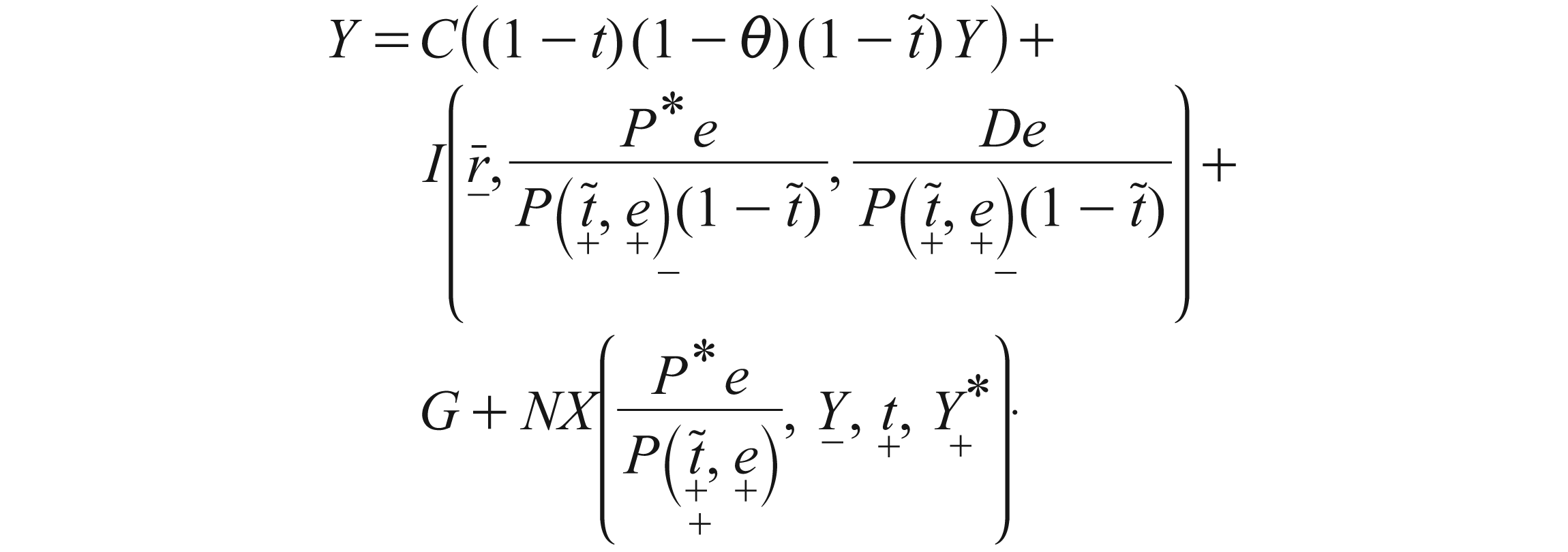
Following the Keynesian tradition, we assume that aggregate output is demand determined. It is given by

Y = C ((1 - t) (1 - θ) (1 - \tilde{t}) Y) + I (\underline{r}, \underline{p}, \underset{​}{\underline{\tilde{D}}}) + G + N X (\underset{+}{\tilde{P}}, \underline{Y}, \underset{+}{t}, \underset{+}{Y^{*}}) .

(1)

In Equation (1), Y is GDP, t is direct tax rate, θ is fixed share of Y that accrues to foreign investors, $\tilde{t}$ is net (of subsidy) indirect tax rate, I is investment, r is the interest rate, $p i s (P^{*} e / P (1 - \tilde{t}))$ , $\tilde{P} i s (P^{*} e / P)$ , P* is foreign price in foreign currency, e is nominal exchange rate and P is domestic price level, $\tilde{D} i s (D e / P (1 - \tilde{t}))$ , where D is stock of external debt of the domestic firms in foreign currency, NX is net export and Y* is GDP of the rest of the world. We assume P* to be given in Indian context. This is because India is a small player in the world market of produced goods and services and, therefore, cannot influence prices of foreign goods prevailing in the world market through its purchases and sales. For similar reasons, Y* is also assumed to be given. Since India is a small player in the world market, it cannot influence foreign GDP through its exports and imports. Incorporation of θ and $\tilde{t}$ in the consumption function, p and t in the investment and net export functions respectively are our innovations. Krugman (1999) identified D as an argument of the investment function. We justify these innovations below.

Let us explain Equation (1). It states that aggregate consumption is an increasing function of disposable income. PY denotes NDP at current market prices. Of this, $\tilde{t} P Y$ is paid out to the government in net indirect taxes. Thus, $(1 - \tilde{t}) P Y$ gives nominal NDP at factor cost and $(1 - \tilde{t}) Y$ gives real NDP at factor cost. Since, in the short run, the fraction of domestic financial and real assets held by foreign investors may be taken as given, it may be sensible to assume that a fixed fraction of non-wage income (which again we assume to be a fixed proportion of Y for simplicity) accrues to foreign investors. Thus, $(1 - θ)(1 - \tilde{t}) Y$ is the national income in real terms. Note that foreigners’ share in NDP at factor cost includes external debt servicing charges, $D {\tilde{r}}^{*} e$ , where ${\tilde{r}}^{*}$ denotes the given foreign rate of interest applicable to D. However, we ignore them for simplicity. If we had considered them explicitly here, θ would have been an increasing function of e, and that would have made our results stronger. Moreover, a bulk of foreign capital flows into domestic financial assets denominated in domestic currency. That is the reason why it is standard in the open economy macroeconomics literature to regard the interest rate differential (the difference between the domestic interest rate and foreign interest rate) and the expected rate of depreciation of domestic currency as the major determinants of foreign capital inflow.

We have already explained the investment function. We have, however, not put in the foreign exchange reserve as an argument in the investment function, since we shall assume a flexible exchange rate here, as it may be more appropriate at the current juncture. There is another important point to note. We have deflated both prices of foreign goods in domestic currency and debt servicing charges in domestic currency not by the domestic market price, but by the domestic price received by the domestic producers given by $(1 - \tilde{t}) P$ . When prices of foreign goods and debt servicing charges in domestic currency rise relative to the prices domestic producers receive (which is given by the market price net of the net indirect tax rate), there takes place profit squeeze and, consequently, erosion of net worth. In calculating firms’ profit, what we have to take into reckoning is not their total revenue in domestic currency, but their total revenue in domestic currency net of net indirect taxes.

The net export function in Equation (1) is standard and does not need any explanation except for the argument, t, and the reason why we have deflated the foreign price level by domestic market price, P. Regarding the first, we think that consumption of the relatively well-to-do sections of people is highly import-intensive, and an increase in the direct tax rate will improve trade balance. In respect of the latter, we must point out that prices relevant for foreign buyers of domestic goods and domestic buyers of foreign goods, that is, for export and import demand, are foreign and domestic market prices as given by P * e and P, respectively.

We assume that the domestic price level, P, is an increasing function of $\tilde{t}$ and e, as they are very important determinants of cost of production in Indian context. Let us explain this. It is common knowledge that in India, indirect taxes constitute a very important source of tax revenue (see GoI, 2014, p. 61) and imported intermediate inputs such as, to name only the most well-known ones, petroleum and petroleum products, fertiliser, electronic components, etc. are essential for production (see GoI, 2014, p. 160). P should also be an increasing function of the money wage rate, W. It may be sensible to assume W to be rigid (non-market clearing) and make it an increasing function of P as well as Y. However, here we assume W to be fixed and do not consider it explicitly as a determinant of P for simplicity and without any loss of generality. We also assume expected rate of inflation to be given and ignore it for analytical convenience. Thus,

P = P (\underset{+}{\tilde{t}}, \underset{+}{e}) \cdot

(2)

Note that here, $P (1 - \tilde{t})$ covers the factor cost including profit and the cost of imported intermediate inputs. An increase in $\tilde{t}$ or e raises P, but it is likely that the adjustment will only be imperfect. This is because most of the non-agricultural sectors are oligopolistic (characterized by the dominance of a few large producers), and oligopolistic interdependence (as captured in the kinked oligopoly model) makes prices sticky, and thereby prevents full pass-through of a cost-push in the short run. The implication of this assumption is that following a rise in $\tilde{t}$ , $(1 - \tilde{t}) P (\tilde{t}, e)$ falls, and an increase in e leads to a rise in $(P^{*} e / P (•) (1 - \tilde{t}))$ .

Using Equation (2), we write the values of p and $\tilde{D}$ as

p = \frac{P^{*} e}{P (\underset{+}{\tilde{t}}, \underset{+}{e}) (1 - \tilde{t})}

(3)

\tilde{D} = \frac{D e}{P (\underset{+}{\tilde{t}}, \underset{+}{e}) (1 - \tilde{t})} \cdot

(4)

Note that given the assumption that adjustments in P are only imperfect with respect to changes in $\tilde{t}$ and e, p and $\tilde{D}$ will rise following an increase in e.

Substituting Equations (3) and (4) into Equation (1), we find that there are three endogenous variables in Equation (1), namely Y, r and e. Let us now focus on the determinants of r and e. Let us consider r first. It is determined in the financial sector. We have made some innovations here too. We specify them below.

The Financial Sector

In the standard Keynesian model referred to above, the financial sector is captured by the money market equilibrium condition, represented by the LM curve. However, as we have already mentioned, the RBI seeks to regulate the interest rate though LAF (by fixing the policy rates such as the repo rate and the reverse repo rate), MSS and OMOs. Hence, following Romer (2000), instead of the LM, we incorporate here the following monetary policy rule or the monetary reaction function of the RBI:

r = \bar{r} \cdot

(5)

Let us explain Equation (5). The RBI regulates interest rates to achieve both growth and inflation targets. In other words, the RBI may follow some kind of a Taylor rule (see Taylor, 1993). However, here we choose not to make interest rate a function of growth rate and inflation (which Romer, 2000 makes) and simply treat it as a policy variable and fixed. The reason is that the RBI normally changes its policy rates after the growth rate and rate of inflation have deviated from their trend and target levels, respectively, and it does so after much deliberation. In other words, RBI’s policy responses are sluggish. Since our focus is on the short run, we consider it appropriate to treat the interest rate as fixed. This will also help us examine how a change in r will affect rates of growth and inflation in India at the current juncture.

Moreover, the RBI may face a policy dilemma in tackling recession—a point that we shall seek to develop in our subsequent research. If the RBI lowers the interest rate to counter recessionary forces, it may induce capital flight, and thereby an increase in the exchange rate, which will generate a cost-push stoking inflation. This may deter the RBI to change the interest rate in times of recession. This is also one reason why we have made interest rate fixed here. This line of reasoning may give a clue as to why the RBI kept its policy rates unchanged until 29 January 2013, even though the current recession had started in the second quarter of 2011–2012, despite immense pressure from the media representing the business lobby and also from the Finance Minister, GoI. Only as late as on 29 January 2013, it announced a modest cut in the repo rate by 25 basis points.

Another point to note here is that the central bank may not be able to control interest rates fully. In the US, for example, following the financial meltdown, borrowing costs to investors rose sharply despite aggressive rate cuts by the FED (see Mishkin, 2009, 2011 in this context). In times of recession, financial intermediaries and lenders become extremely cautious in their lending, credit standards tighten, risk premium on loans goes up sharply and there takes place flight to quality (see Bernanke, Gertler, & Gilchrist, 1996 in this context). However, we disregard this issue of RBI’s inability to regulate interest rate for simplicity. We think that if we incorporate these factors, our results will become stronger. Moreover, in India, the central bank has much stronger control over interest rates, since most of the banks are owned by the government. This is particularly so, since in India, the Ministry of Finance and the RBI act in consonance with one another.

Substituting equations (3), (4) and (5) into Equation (1), we write it as

\begin{array}{l} \begin{matrix} Y = C ((1 - t) (1 - θ) (1 - \tilde{t}) Y) + \end{matrix} \\ \begin{matrix} I (\underline{\bar{r}}, \underline{\frac{P^{*} e}{P (\underset{+}{\tilde{t}}, \underset{+}{e}) (1 - \tilde{t})}}, \underset{​}{\underline{\frac{D e}{P (\underset{+}{\tilde{t}}, \underset{+}{e}) (1 - \tilde{t})}}}) + \end{matrix} \\ \begin{matrix} G + N X (\underset{+}{\frac{P^{*} e}{P (\underset{+}{\tilde{t}}, \underset{+}{e})}}, \underline{Y}, \underset{+}{t}, \underset{+}{Y^{*}}) ​ \cdot \end{matrix} \end{array}

(6)

We find from Equation (6) that aggregate planned demand as given by the RHS of the equation and which we shall denote by E is a function of e and Y, given the exogenous variables such as $t, \tilde{t}, \bar{r}$ , and Y* among others. We thus rewrite Equation (6) as

Y = E (\underset{+}{Y}, \underline{e}; \underline{\tilde{t}}, \underline{\bar{r}}, \underline{t}, {\underset{+}{Y}}^{*}), 0 \leq E_{Y} \leq 1.

We can rewrite the above equation as

\begin{matrix} \tilde{E} = \tilde{E} (\underline{Y}, \underline{e}; \underline{\tilde{t}}, \underline{\bar{r}}, \underline{t}, {\underset{+}{Y}}^{*}) = 0 \\ \tilde{E} \equiv E - Y \Rightarrow \tilde{E} ​_{Y} = E ​_{Y} - 1 \leq 0 \cdot \end{matrix}

(7)

Let us explain Equation (7) using Equation (6). An increase in Y raises disposable income, improves capacity utilization and profit and thereby raises both C and I. It, however, reduces NX. In the net, we assume that, as standard, _EY lies between zero and unity. Hence, $\tilde{E} _{Y} \leq 0$ . An increase in e raises prices of foreign goods in terms of domestic currency. It also generates a cost-push, and thereby raises P. However, given the oligopolistic structures in most markets, there is unlikely to be a full pass-through of an increase in e in the short run, leading to an imperfect adjustment in P and a profit squeeze. Thus, it is reasonable to assume that both p and $\tilde{D}$ increase, following an increase in e. Since production and investment in India are heavily import dependent, an increase in e makes both government and business nervous, leading to policy paralysis and dampening of investor sentiment—a point which we have discussed in detail earlier. NX improves mainly owing to the reduction in investment demand, given very low price elasticity of both import and export (RBI, 2012). The latter is due to a very high import intensity of Indian export (RBI, 2012). Thus, even though an increase in e raises NX, in Indian context, which we have explained above, it is reasonable to assume that its demand depressing effect not only dominates, but it does so significantly. This explains the sign of the partial derivatives of E and $\tilde{E}$ with respect to e.

An increase in $\tilde{t}$ lowers C by reducing disposable income. It also decreases the price received by domestic producers, as there is unlikely to be a full pass-through of the increase in $\tilde{t}$ . Hence, both p and $\tilde{D}$ decline, producing a dampening effect on investment. It also reduces NX by making domestic goods dearer relative to foreign goods. Hence, an increase in $\tilde{t}$ lowers E and $\tilde{E}$ . Signs of other partial derivatives of Equation (7) are quite self-evident from Equation (6).

Let us now turn to the determination of e. The BOP consists of trade surplus and net inflow of foreign capital, which we shall denote by F. Given the restrictions on capital inflow in India, capital is imperfectly mobile. In open economy macroeconomics literature, see, for example, Romer (1996), it is standard to assume that F depends upon interest rate differential and expected rate of depreciation of the domestic currency. In Indian context, given recent experiences with foreign capital inflows, it may be appropriate to assume that the expected rate of depreciation of domestic currency depends crucially on the sovereign rating assigned by the credit rating agencies to the domestic economy. Let us elaborate this. In the Union Budget for the year 2012–2013 placed in the parliament at the end of February 2012, GoI introduced ‘general antiavoidance rule’ (GAAR). At the same time, it brought about a ‘retrospective amendment to the Income Tax Act pertaining to indirect transfer of Indian assets’. Both these measures implied an increase in the tax rate applicable to foreign investors’ income from their investments in India. Immediately, the credit rating agencies swung into action. Standard and Poor (S&P) downgraded India’s sovereign rating in April 2012 and threatened to downgrade it further to junk status. Other credit rating agencies such as Moody’s and Fitch also followed suit. Following this rating downgrade, there took place a drastic decline in the inflow of foreign capital in the first quarter of 2012–2013—see Table A4. In a press statement released on 15 May 2012 (GoI, Ministry of Finance, Press Information Bureau, 2012), GoI stated: ‘However, all the SCRAs (Sovereign Credit Rating Agencies such as Moody’s Investor Services, Standard & Poor’s, Fitch Ratings etc.) have not favourably commented on India’s fiscal deficit and debt’. In their April 2012 report, S&P had revised the outlook on the long-term rating on India from stable to negative. In its report, S&P also stated that the outlook has been revised ‘to reflect at least a one-in-three likelihood of a downgrade if the external position continues to deteriorate, growth prospects diminish, or progress on fiscal reforms remains slow’.

With the rating downgrade, there took place a large decline in capital inflow and, consequently, a shooting up of the exchange rate (from ₹49 in February 2012 to ₹56 in June and ₹55 in July 2012—see Table A1). GoI grew terribly nervous and started adopting since 12 September 2012 a slew of measures to appease the foreign investors and the credit rating agencies. On 12 September 2012, GoI allowed, for example, FDI in retail and promised more reforms on this line. It also brought about a steep increase in the administered prices of diesel and cooking gas. The measures were obviously so detrimental to the interest of the poor that it evoked a nation-wide protest. The protest was so true and forceful that the Prime Minister (PM) of India had to address the nation to explain why such harsh measures were necessary to reverse the economic slowdown. It may be instructive to quote a few portions of the speech the PM delivered on 21 September 2012.

We are at a point where we can reverse the slowdown in our growth. We need a revival in investor confidence domestically and globally. The decisions we have taken recently are necessary for this purpose. Let me begin with the rise in diesel prices and the cap on LPG cylinders….If we had not acted, it would have meant a higher fiscal deficit. If unchecked this would lead to…a loss of confidence in our country. The last time we faced this problem was in 1991. Nobody was willing to lend us even small amounts of money then…. I know what happened in 1991 and I would be failing in my duty as Prime Minister of this great country if I did not take strong preventive action.

The scenario delineated above clearly brings out the importance of the credit rating agencies at the current juncture. It follows from the above that their rating depends upon domestic government’s attitude towards foreign investors as reflected in the tax rate that it seeks to apply to foreign investors’ income, the level of restrictions it puts on foreign investments, etc. Denoting the sovereign rating assigned by the credit rating agencies to the domestic economy by ρ, we make it a decreasing function of the tax rate applied to foreign investors’ income (τ) and the level of restrictions on foreign investments (denoted R). An increase in R implies an increase in the level of such restrictions. Finally, there may be many exogenous factors that may influence F. We, therefore, incorporate an exogenous variable ϕ as a determinant of F. An increase in ϕ is assumed to imply an improvement in the perception of foreign investors regarding India for extraneous reasons, which may or may not be political in nature. Thus,

F = F ([{\underset{+}{\bar{r} - r}}^{*}], \underset{+}{ρ} (\underline{τ}, \underline{R}), \underset{+}{ϕ}) \cdot

(8)

Let us explain the meaning of R a little more. There are legal restrictions on both foreign direct investment (FDI) and FPI. There are legal barriers to entry into different sectors, such as, for example, multibrand retail. Similarly, there are legal caps. GoI and RBI have imposed restrictions on both FDI and FPI. There are sectoral ceilings or caps on FDI, and this cap varies across sectors. For details, one can go through GoI (2013). RBI also has imposed restrictions on FPI. There are caps on the amounts that Foreign Institutional Investment (FIIs) can invest in any Indian company. An increase in R means a relaxation of these caps or barriers to entry. Despite these caps, foreign capital inflows are sensitive to interest rate differential and other economic variables because these caps are not binding at least in some sector, that is, at least in some sectors, the levels of foreign investments considered optimal by foreigners are below their respective caps.

In Equation (8), the first determinant of F is the interest rate differential, $(\bar{r} - r^{*})$ , of which, r* denotes the foreign rate of interest, which is given to the domestic economy. Let us now specify the equilibrium condition in the foreign exchange market. We assume the exchange rate to be flexible for reasons we have already explained. The following BOP equilibrium condition determines the exchange rate:

N X (\underset{+}{\frac{P^{*} e}{P (\underset{+}{\tilde{t}}, \underset{+}{e})}}, \underline{Y}, {\underset{+}{Y}}^{*}, \underset{+}{t}) + F (\underset{+}{[\bar{r} - r^{*}]}, \underset{+}{ρ} (\underline{τ}, \underline{R}), \underset{+}{ϕ}) = 0 ​ \cdot

(9)

The LHS of Equation (9) gives the BOP, which we shall denote by B. We find from Equation (9) that it is a function of Y, e and the exogenous variables such as $\bar{r}, \tilde{t}, τ, Y^{*}$ and t, among others. We thus rewrite Equation (9) as

B (\underline{Y}, \underset{+}{e}; \underline{\tilde{t}}, \underset{+}{ϕ}, \underline{τ}, {\underset{+}{Y}}^{*}, \underset{+}{t}, \underset{+}{\bar{r}}, \underline{R}) = 0 ​ \cdot

(10)

Let us now explain Equation (10) using Equation (9). A ceteris paribus increase in Y reduces net exports, and thereby lowers B. Again, an increase in e, as we have pointed out earlier, raises $(P^{*} e / P)$ . As a result, for reasons we have already explained, NX and, therefore, B go up. An increase in $\tilde{t}$ reduces NX by making domestic goods dearer, and thereby reduces B. Signs of other partial derivatives of B(•) are quite self-evident from Equation (9).

The specification of our model is now complete. It contains two key equations, namely Equations (7) and (10) in two unknowns, namely Y and e. We can, therefore, solve these equations for the equilibrium values of the two endogenous variables. The solution of Equations (7) and (10) is shown in Figure 1, where e is measured on the vertical axis and Y on the horizontal axis. The lines YY and BB represent Equations (7) and (10), respectively, in Figure 1. The equilibrium corresponds to the point of intersection of the two lines. We are now in a position to use this simple model to shed light on India’s recent macroeconomic experiences.

Figure 1.

Determination of Y and e

Before proceeding further, it may be instructive to explain how the model we have developed can shed light on fluctuations in short-period or year-on-year growth rates. Actual short-period growth rates (annual, quarterly, etc.) usually deviate from their trend values. If in some years at a stretch, actual annual growth rates are perceptibly above (below) their trend values, they are referred to as years of boom (recession). Short-period macro models, micro-founded or otherwise, explain these deviations of actual short-period growth rates from their trend values. A short-period model determines macro variables such as Y and P of a given short period (year, quarter, etc.), which we may refer to as period t. Determination of Y and P in period t amount to the determination of the growth rate of Y and the rate of inflation from period t – 1 to period t, since in period t, the levels of Y and P that are obtained in period t – 1 are known and, therefore, given. A short-period Keynesian model, for example, which determines Y in any given short period as a function of, among others, the autonomous component of aggregate demand, explains fluctuations in the short-run growth rates of an economy in the following manner. It shows that if there occurs a favourable demand shock in period t, that is, if the autonomous component of aggregate demand (the component of aggregate demand that is independent of the values of the endogenous variables of the model) is above the level that would have made the actual growth rate of Y from period t-1 to period t equal to its trend value (charted out by the data of actual short-period growth rates of past periods), the value of Y in period t would be such that the actual growth rate from period t – 1 to period t will be above its trend value. Thus, the short-period model we have developed is used to explain why in India, the actual annual growth rate in 2003–2004 was higher than that in 2002–2003, that is, why the value of Y in 2003–2004 was above the level that would have made the annual growth rate in 2003–2004 equal to that in 2002–2003. In this context, a quote from Romer (2000, pp. 157–158) may be instructive. It says,

[I]n the traditional AD–AS approach, the aggregate demand curve relates the price level and output. One therefore has to explain that the model implies that a negative aggregate demand shock does not actually lead to a lower price level, but to a price level lower than it otherwise would have been. This point is omitted altogether in some treatments. Even when it is explained, it is sufficiently subtle that many students end up confused about the model’s predictions or about the distinction between the price level and inflation.

Spurt in the Growth Rate in 2003–2004

Let us first seek to explain the spurt in the growth rate in 2003–2004. This we do in terms of an exogenous increase in ϕ, which brings about an increase in F for extraneous reasons. In fact, Table A1 shows that there did take place almost trebling of foreign investment inflows in 2003–2004 for no apparent reasons, at least in Indian context. Our model yields the following theorem regarding the effect of an increase in ϕ on Y and e:

Theorem 1: An increase in ϕ will raise Y and lower e.

We prove this theorem in A.2 in the appendix. Let us illustrate the theorem graphically.

From Equation (9), it follows that an increase in F brought about by a rise in ϕ will lower B, given Y, e and all other exogenous variables. To keep BOP in equilibrium, e has to be lowered, given Y—see Equation (10). BB in Figure 1, therefore, shifts downwards. YY, however, stays unaffected—see Equation (7). Y will thus tend to rise and e will tend to fall. The increase in ϕ and the rise in F that it brings about improve OP situation and start lowering e making imported intermediate inputs and capital goods cheaper. External debt servicing charges decline too. This improves margins and also gives a boost to business and government confidence as regards sustainability of larger imports at lower cost and, therefore, higher growth. Credit standards loosen, there takes place speedier clearances of investment applications and investment goes up—see Equations (6) and (7). Thus, the decline in e induces an increase in Y. Thus, growth rate picks up.

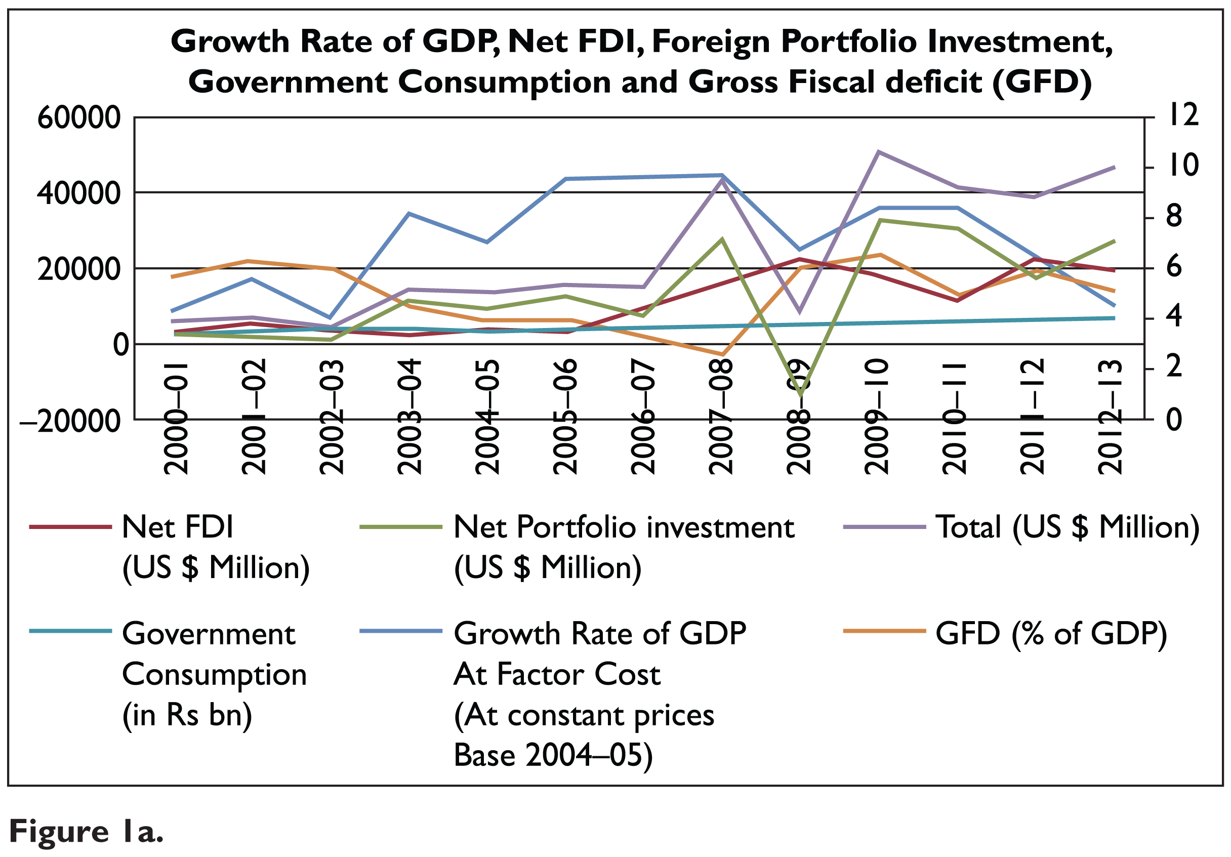
Our model also predicts—one can work it out quite easily—a decline in fiscal deficit as a proportion of GDP—since receipts rise in the same proportion as Y, but expenditures do not. This happens if fiscal policy is not avowedly expansionary, and it was not so during 2003–2004. Table A1 shows that gross fiscal deficit as a percentage of GDP did decline from 5.91 in 2002–2003 to 4.48 in 2003–2004.

Dip in the Growth Rate in 2008–2009 and the Recovery in 2009–2010

In 2008–2009, just the opposite happened. ϕ decreased, that is, for exogenous reasons, F declined—see Table A1. Accordingly, as predicted, there took place a rise in the exchange rate, a decline in growth rate and an increase in fiscal deficit as a proportion of GDP (of course, during this period, fiscal policy became avowedly expansionary)—see Tables A1 and A2 and also the adjoining Figures 1a and 2. Similarly, we can explain the experiences of 2009–2010 in terms of an increase in ϕ. In this case, fiscal deficit as a proportion of GDP increased, despite an increase in growth rate because of the expansionary fiscal policy pursued by the government.

Recession in 2011–2012

India entered into recession again since the second quarter of 2011–2012—see Table A1. The reason perhaps was different from that in 2008–2009. The recession, according to RBI (2012), was on account of a ‘slackening of export growth owing to a slowdown in external demand’. According to RBI, therefore, export declined (below its trend value) in 2011–2012 as a result of a fall in Y* (below its trend value). Let us see how it affects the macro variables using our model. Our model yields the following theorem:

Figure 1a.

Figure 3.

Theorem 2: A decline in Y* brings about a decline in Y and a rise in e.

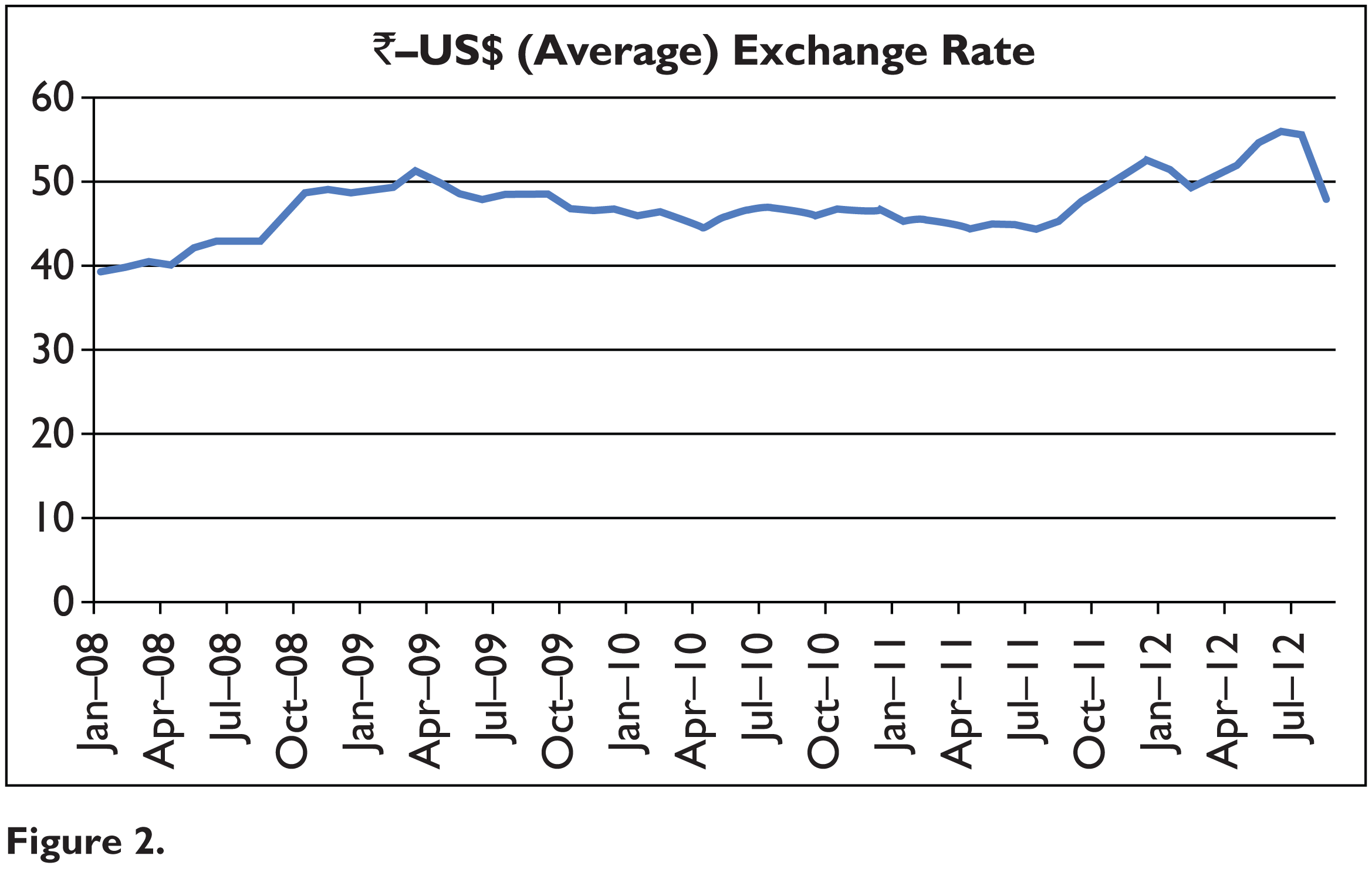
This theorem is proved in A.3 in the appendix. Let us illustrate this theorem graphically. A decline in Y* brings about a decrease in E, given Y, e and other exogenous variables—see Equation (7). Therefore, as follows from Equation (7), YY shifts leftward in Figure 1. B declines too, following a ceteris paribus fall in Y*, given Y, e and other exogenous variables—see Equation (10). Hence, as follows from Equation (10), BB in Figure 1 shifts leftward too. We have proved in A.3 in the appendix that the leftward shift in BB is larger than that in YY, so that in the new equilibrium, Y and, therefore, the growth rate are low, and e higher. The way the changes mentioned above happen may be the following. In the wake of the decline in Y* and the consequent decrease in net export, BOP deficit emerges sending e northward. The rise in e makes both the government and business jittery for reasons we have already explained dampening investment and thereby import demand. The excess supply in the goods market induces shrinkage in Y. This prediction is consistent with the data presented in Tables A1 and A2, where we find that the growth rate fell from 8.4 per cent in 2010–2011 to 6.5 per cent in 2011–2012, and the exchange rate in 2011–2012 rose from ₹44.9045 in May 2011 to ₹52.6769 in December 2011 and then fell to ₹49.1671 in February 2012. The decline in e from December to February may be explained as standard in terms of relative speeds of adjustments of e and Y. Initially, the burden of adjustment of the exogenous fall in NX was borne principally by e. It rose to correct the BOP deficit overshooting its new equilibrium value. Later, Y started declining, improving BOP situation, and thereby pulling down e towards its new equilibrium value. Finally, our model predicts an increase in fiscal deficit as a proportion of Y, with a fall in Y. In consonance with this prediction, as we find from Table A1, fiscal deficit did increase from 4.87 per cent of GDP in 2010–2011 to 5.89 per cent of GDP in 2011–2012 because of the slackening of the growth rate, despite efforts at fiscal correction. We can thus explain the changes in the major macro variables in 2011–2012 using our model.

The Deepening of Recession in 2012–2013 and the Impending Crisis

The recession deepened in 2012–2013. The growth rate declined from 6.5 per cent in 2011–2012 to 5 per cent in 2012–2013. The exchange rate resumed its upward journey. It rose from ₹49.1671 in February 2012 to ₹55.4948 in July 2012—see Table A2. Both Wholesale Price Inflation (WPI) inflation and Consumer Price Inflation (CPI) inflation rose up. Despite determined efforts at fiscal correction, fiscal deficit as a percentage of GDP went up. In our view, the deterioration in the macroeconomic performance of the Indian economy in 2012–2013 was to a large extent due to the GAAR announced in the Union Budget in February 2012 (GoI, 2012) along with the retrospective amendment to the income tax law pertaining to indirect transfer of Indian assets. In terms of our model, these measures led to an increase in τ. The rise in τ dealt a body blow to foreign investment inflows. There took place a substantial decline in F in the first quarter of 2012–2013—see Table A4. Let us now see whether we can attribute the deterioration in India’s economic performance to increases in τ using our model.

Theorem 3: An increase in τ will lower Y and raise e.

The theorem is proved in A.4 in the appendix. We illustrate the theorem graphically below. Following an increase in τ, as follows from Equation (10), B declines, corresponding to any given (Y, e). Hence, BOP will be in equilibrium at a higher e, corresponding to any given Y or at a lower Y, corresponding to any given e—see Equation (10). Thus, BB in Figure 1 will shift upwards or to the left. YY schedule, however, remains unaffected. Hence, in the new equilibrium, e will be higher and Y lower. This result can easily be derived mathematically. It is also perfectly in accord with what happened in the first quarter of 2012–2013. The result may be explained as follows. An increase in τ reduces capital inflow leading to a BOP deficit and, consequently, an upward movement in e. This rise in e through the channels mentioned earlier depresses demand for goods and services, and thereby exerts downward pressure on Y.

Foreign investors and the credit rating agencies responded sharply to the measures that brought about an increase in τ. S&P downgraded India’s sovereign rating in April, and again in June, it threatened to downgrade India’s sovereign rating to junk status. All other major credit rating agencies followed suit. Commensurately, there took place a very substantial decline in the net inflow of foreign investments in Q1 of 2012–13 (see Table A4). As predicted by our model, this very large decline in foreign investment brought about a significant decline in the growth rate and sent the exchange rate soaring. This unnerved the Union Government, as the possibility of an explosive currency crisis loomed large. It took steps to give strong signals to the foreign investors that it was going to reverse the anti-foreign investment measures. One signal, for example, went in the form of removal of the finance minister responsible for the 2012–2013 budget from the finance ministry. Besides this, since September 2012, GoI started adopting a slew of measures to restore foreign investors’ confidence, and thereby stabilizing foreign investment inflows. ‘These reforms include, inter alia, liberalized FDI norms for the retail, insurance and pension sectors, a road map for fiscal consolidation and an increase in FII limits in the corporate and government debt markets’ (RBI, 2013c). The major plank of fiscal consolidation consisted in a substantial hike in the administered price of diesel and cooking gas. GoI also declared that diesel price would be gradually raised further and subsidy would eventually be removed. GoI also postponed the implementation of GAAR and retrospective amendment of income tax laws. Buoyed by these signals, foreign investments bounced back in Q2 (see Table A4). But, despite the reversal in foreign capital inflow, rupee continued to depreciate (see Tables A5 and A6), and there was no let-up in recession—see Table A1. In sum, macroeconomic health of India continued to deteriorate, despite the reversal in the net foreign capital inflows. Why did this happen? The answer, in our view, lies in the measures adopted by the GoI to tackle the crisis created by the decline in the net inflow of foreign capital. We explain our position below.

Assessment of the Fiscal Measures Adopted by the Government to Resolve the Crisis

A hike in the administered prices of diesel and cooking gas reduced the rate of subsidy. In our model, these measures led to an increase in $\tilde{t}$ . In fact, in the budget for the financial year 2012–2013, the GoI also proposed to reduce subsidies and to raise excise and service tax rates by 2 per cent. In the rail budget in February 2012 (GoI, 2012), passenger fares and freight charges were raised. Electricity tariffs were also raised. All these measures in our model amount to a raising of $\tilde{t}$ . Relaxation of controls over foreign direct and portfolio investments implies a fall in R. Thus, since September 2012, $\tilde{t}$ was raised and τ and R were lowered. In what follows, we shall use our model to derive the impact of a rise in $\tilde{t}$ and a decline in R.

Let us now examine how an increase in $\tilde{t}$ is likely to affect the macro variables. Following a rise in $\tilde{t}$ , as follows from Equation (7), E goes down, corresponding to any given (Y, e), given all other exogenous variables. Therefore, the goods market will be in equilibrium at a lower Y, corresponding to any given e or to a smaller e, corresponding to any given Y—see Equation (7). Thus, YY shifts downwards or to the left. It also creates a BOP deficit, corresponding to any given (Y, e)—vide Equation (10). The BOP, as follows from Equation (10), will be in equilibrium at a lower Y, given e, or at a smaller e, given Y. Thus, BB in Figure 1 will also shift upwards or to the left. In the new equilibrium, therefore, Y will be less unambiguously, but e may change in either direction. However, we shall focus on the case, where e becomes higher in the new equilibrium, as it fits Indian data. It is quite clear from Figure 1 that if the magnitude of the horizontal shift in BB is larger than that in YY, e will rise. Otherwise it will either stay unchanged or fall. In A.4 in the appendix, we have derived this result mathematically and also the magnitudes of horizontal shifts in BB and YY—see (a.7) and (a.8). We find that if marginal propensities to save and invest are sufficiently large and small respectively, the dampening effect of a rise in $\tilde{t}$ on aggregate demand is not sufficiently strong and foreign capital inflow does not respond much to an increase in $\tilde{t}$ , the absolute value of the horizontal shift in BB will be larger than that in YY and e will rise. This yields the following theorem:

Theorem 4: An increase in $\tilde{t}$ lowers Y unambiguously, but its impact on e is ambiguous. It will raise e if the contractionary effect of an increase in $\tilde{t}$ on aggregate demand for goods and services is sufficiently small and the marginal propensity to save is sufficiently large.

This theorem, as we have already mentioned, is proved in A.5 in the appendix.

Intuitively, an increase in $\tilde{t}$ creates BOP deficit by making domestic goods dearer. However, it also directly reduces demand for Y, putting a downward pressure on Y. The consequent fall in Y will tend to improve the BOP situation. If the latter effect is not strong enough, there will emerge BOP deficit at the initial equilibrium exchange rate. Exchange rate will accordingly rise, depressing investment for reasons we have already explained. Thus, the rise in e puts downward pressure on Y. Thus, a rise in $\tilde{t}$ may lead to recession, a rise in the exchange rate. Moreover, both the increase in the exchange rate and the rise in $\tilde{t}$ will engender an increase in the inflation rate. Thus, the effects produced by the increase in τ may be reinforced by the rise in $\tilde{t}$ . Thus, the continuation of recession and the resumption of the northward journey of the exchange rate are of no surprise in the Q1 of 2012–2013. Propelled by the increases in $\tilde{t}$ and e, the price level also increased, generating inflationary pressure (see Table A3).

The Effect of a Decrease in R

As we have pointed out above, since September 2012, the GoI started relaxing controls over foreign direct and portfolio investments. This implies a decline in R in our model. Let us now examine how a reduction in R affects Y and e in our model. We have derived formally the following theorem in section A.6 in the appendix.

Theorem 5: A reduction in R will raise Y and lower e.

Here, we shall derive the above theorem graphically. Since R is not a parameter in the goods market equilibrium condition Equation (6), the YY schedule in Figure 1 remains unaffected. Let us now focus on the BB schedule. A reduction in R corresponding to any (Y, e) on the initial BB schedule will lead to an increase in F, and thereby engender BOP surplus. Therefore, corresponding to any given e, the BOP will be in equilibrium at a larger Y. Hence, the BB schedule in Figure 1 will shift to the right. Hence, in the new equilibrium, Y will be higher and e lower. The intuition of the result is quite easy to explain. Following a lowering of R, there takes place an increase in the net inflow of foreign capital generating a BOP surplus at the initial equilibrium (Y, e). Hence, e will begin to fall, putting an upward pressure on Y. This process of fall in e and increase in Y will continue until the BOP becomes zero again. The fall in e will also soften the inflation rate.

Let us now go back to India’s macroeconomic scenario in 2012–2013. Despite the favourable effects produced by the reduction in τ and R, the growth rate slid below the level of the previous fiscal; BOP situation deteriorated, bringing about a large increase in the exchange rate. There also took place a noticeable increase in the inflation rate. Our analysis of the effects that different policy parameters such as τ, R and $\tilde{t}$ produce strongly suggest that the deteriorating macroeconomic health of India was due to the steep increase in the net indirect tax rate $\tilde{t}$ that the GoI brought about in 2012–2013. It adversely affected both growth and BOP, and its unfavourable effects dominated the favourable effects of the reduction in R and τ.

It is clear from above that India’s macroeconomic health depends crucially on external factors. A global recession or a capital flight due to hostile domestic policies or favourable policies or prospects in foreign countries sends India into a recession with BOP difficulties that lead to a soaring of the exchange rate, which, in turn, generates inflationary pressure by producing a cost-push. We have seen above that a cut in subsidy through hikes in administered prices of crucial inputs or raising of indirect tax rates may reinforce the adverse effects, instead of countering them. This was perhaps the case in India in 2012–13. We have to, therefore, explore other policy options to counter the adverse effects produced by deterioration in the external environment. We shall now examine how a hike in the personal income tax rates along with a suitable expenditure policy affects Y and e in our model.

The Effect of an Increase in the Personal Income Tax Rate Combined with an Increase in G

Here, we consider a policy where the government raises personal income tax rate and also its consumption or investment expenditure in such a manner that the value of aggregate demand at the initial equilibrium values of Y and e remains unaffected. We have derived formally the impact of this policy on Y and e in section A.7 in the appendix. It yields the following theorem:

Theorem 6: A hike in the personal income tax rate t accompanied by such an increase in G that the level of aggregate demand for goods and services at the initial equilibrium (Y, e) remains unchanged will bring about an increase in Y and a fall in e.

Here, we derive this theorem graphically. Following a ceteris paribus increase in t by dt, the amount of consumption demand corresponding to any given (Y, e) falls by $C^{'} . (1 - θ) (1 - \tilde{t}) Y d t$ and net export rises by NX_tdt leading to a fall in aggregate demand by $C^{'} . (1 - θ) (1 - \tilde{t}) Y d t - N X _{t} d t$ . Hence, G has to increase by the same quantity to keep aggregate demand unaffected, corresponding to any given (Y, e). Obviously, this policy will leave the YY schedule unaffected. Let us now focus on the BB schedule. Following an increase in t by dt, net export rises, improving the BOP situation. Hence, corresponding to any (Y, e) on the initial BB schedule, there is now a BOP surplus. Hence, corresponding to any e, the BOP will be in equilibrium at a larger Y. Thus, the BB schedule in Figure 1 will shift to the right. Therefore, Y will rise and e will fall. This is the kind of impact that is necessary to counter the adverse effects produced by deterioration in the external environment. It will soften inflation rate and also reduce fiscal deficit.

Conclusion

This article argues on the basis of the available evidences that India’s recent growth performance is determined by external factors. After a careful scrutiny of data, this article attributes the remarkable increase in India’s growth rate in 2003–2004 to a sharp increase in the net inflow of foreign capital. It also identifies a noticeable decline in the net inflow of foreign capital as the cause for the dip in the growth rate in 2008–2009. It also explains the recession in the year 2011–2012 and in the first quarter of 2012–2013 in terms of a global recession induced decline in export demand and a large reduction in net capital inflow, respectively. The article also shows that a decline in export demand due to a global recession or a reduction in the net capital inflow not only reduces the growth rate, but also sends the exchange rate, and thereby soaring the inflation rate. In 2012–2013, the GoI cut down on subsidies and raised indirect tax rates to neutralize the adverse impact produced by the fall in the net inflow of foreign capital that occurred in the first quarter. The article shows that the impact of this kind of a policy may be stagflationary. For this reason, the article attributes the continuation of the stagflationary situation all through the rest of 2012–2013, despite the revival of net capital inflows since the second quarter of 2012–2013 to the policy of reduction in subsidies and raising of indirect tax rates. This naturally leads to the question as to which policy the government should adopt to counter the stagflationary forces produced by deterioration in the external environment. This question is of paramount importance at the current juncture, since external factors play a crucial role in determining India’s macroeconomic health. This article shows that a hike in the personal income tax rates coupled with a suitable increase in public consumption or investment expenditure will raise growth rate and lower exchange rate. The latter, in turn, will soften the inflation rate. Thus, this policy seems to be appropriate at the current juncture to revive Indian economy.

Footnotes

Appendix

References

Bernanke

, Gertler

, & Gilchrist

(1996, February). The financial accelerator and flight to quality. The Review of Economics and Statistics, 78(1), 1–15.

Bhagwati

N. J.

(1998). The capital myth: The difference between trade in widgets and dollars. Foreign Affairs, 77(3), 7–12.

GoI (Government of India). (2012). Press Note (May 15), Concern of Credit Rating Agencies on Indian Economy. New Delhi: Ministry of Finance, GoI.

GoI (Government of India). (2014). Union Budget of India 2012–13. New Delhi: Ministry of Finance, GoI.

Korinek

(2010, November 4–5). Hot money and serial crises. Paper presented at the 11th Jacques Pollack Annual Research Conference, Washington, DC.

Krugman

(1999). Balance sheets, the transfer problem, and financial crises. International Tax and Public Finance, 6(4), 459–472.

Mishkin

F. S.

(2009, January). Is monetary policy effective during financial crises? (NBER Working Paper No. 14678). Cambridge, MA: National Bureau of Economic Research.

Mishkin

F. S.

(2011). Over the cliff: From the subprime to the global financial crisis. Journal of Economic Perspectives, 25(1/Winter), 49–70.

Nagraj

(2013, May 18). India’s dream run—2003–08. Economic & Political Weekly, 48(20), 39–51.

10.

RBI (Reserve Bank of India). (2012). The external sector. Macroeconomic and Monetary Development Second Quarter Review (pp. 16–22).

11.

RBI (Reserve Bank of India). (2013a, September 16). India’s foreign trade (Table 127). In Handbook of statistics on Indian economy. India: RBI.

12.

RBI (Reserve Bank of India). (2013b, October 28). The external sector. Macroeconomic and Monetary Policy Review (pp. 14–19).

13.

RBI (Reserve Bank of India). (2013c). Macroeconomic and Monetary Development Third Quarter Review.

14.

Rodrik

(1998). Who needs capital account convertibility. In Kenen

(Ed.), Essays in international finance (pp. 55–65). Princeton, NJ: Princeton University Press.

15.

Romer

(1996). Advanced macroeconomics. New York: The McGraw-Hill Companies Inc.

16.

Romer

(2000). Keynesian macroeconomics without the LM curve. Journal of Economic Perspectives, 14(2/Spring), 1449–1469.

17.

Taylor

J. B.

(1993). Discretion versus policy rules in practice. Carnegie-Rochester Series on Public Policy, 39(1), 195–214.