A Macroeconomic Model with Price Flexibility

Abstract

A simple macroeconomic model is used to show that the market failure to maintain macroeconomic stability can be due to (a) price rigidity or (b) price flexibility that allows false and abnormal prices to prevail. The macroeconomic literature typically considers the first case only; this article focuses on the second case. Besides the Keynesian fiscal policy, this article considers a Pigouvian tax–subsidy scheme; the latter can be used to correct each false price individually (this use in macroeconomics resembles the more familiar use in public economics). This helps alleviate the scarcity of instruments with policymakers. As in the writings of Keynes, price stability (or rigidity) here is a policy target rather than an assumption in the model. There has been a general need to reconsider macroeconomic models since the Great Recession of 2008; this article contributes in this endeavour.

JEL: E12, E62, H20

Keywords

Macroeconomic fundamentals price rigidity false prices Pigouvian tax–subsidy

Introduction

There is a sense of disenchantment with the current state of macro-economic models. Consider the following quote,

Current core—by which I mainly mean the so-called dynamic stochastic general equilibrium [DSGE] approach—has become so mesmerized with its own internal logic that it has begun to confuse the precision it has achieved about its own world with the precision that it has about the real one. This is dangerous for both methodological and policy reasons. … we should be in “broad-exploration” mode. (Caballero, 2010)

This view was expressed after the financial crisis which occurred in and around the year 2007. So it is understandable that there was frustration with the macroeconomic literature. However, there were serious concerns with macroeconomic models even before the crisis. Mankiw (2006) wrote, ‘From the standpoint of macroeconomic engineering, the work of the past several decades looks like an unfortunate wrong turn.’ Some concern was shared by even a leading mainstream macro-economist, Michael Woodford. He wrote, ‘In fact they [DSGE models] have been put to use, only not with such radical consequences as had once been expected’ (Woodford, 2009).

Another expression of dismay was as follows: ‘Training in “state-of-the-art” macroeconomic modelling is “a privately and socially costly waste of time and resources”’ (Buiter, 2009). Consider yet another view: ‘I do not think that the currently popular DSGE models pass the smell test’ (Solow, 2010). Also, the macroeconomic models have not been found useful among the practitioners. Noha Smith expressed the view in 2014 that DSGE fails the market test. The title in Fair (2012) is ‘Has Macro progressed?’ and the author’s answer is, broadly speaking, in the negative.

Given the state of the macroeconomic literature, it is not surprising then that there is also some concern about the achievements of the Federal Reserve System (FED) in maintaining macroeconomic and financial stability. A strong comment was made by Milton Friedman, a Nobel laureate and author of the voluminous book, A Monetary History of the United States. He wrote, ‘No major institution in the U.S. has so poor a record of performance over so long a period, yet so high a public reputation’ (Friedman, 1988). It is interesting that this was written long before the Great Recession and the financial crisis in and around the year 2007. A more recent empirical study concludes that

the Federal Reserve System [in its nearly 100 years of existence] has … tended to err on the side of inflation … That deterioration has not been compensated for, to any substantial degree, by enhanced stability of real output. Although a genuine improvement did occur during … the “Great Moderation,” that improvement, besides having been temporary, appears to have been due mainly to factors other than improved monetary policy. Finally, the Fed cannot be credited with having reduced the frequency of banking panics …. (Selgin, Lastrapes, & White, 2012)

All this motivates a somewhat fresh look at macroeconomics. It may help to begin with first principles. The focus of this article will be on one aspect, namely, the treatment of prices in macroeconomic models. It appears that that there are four different views regarding prices in macroeconomics.

First, prices hardly matter in macroeconomics. This view is implicit in writings that emphasize aspects such as the role of animal spirits in determining investment, coordination failures and the Keynesian cross-diagram (the last one particularly in courses on principles of macro-economics). Second, prices matter but these can be downwards rigid. So, they cannot be an important part of the adjustment mechanism. Downwards rigidity can also take the form of the zero lower bound in case of the interest rate. Finally, it can take the form of fixed exchange rates in the case of open economy models. Third, prices are flexible. This can help but the flip side is that a big departure from prevailing prices or normal prices matters. This view is associated with Fisher (1933) and possibly Keynes (1925). In Lucas (1972) too, a departure from the prevailing prices matters. Fourth, prices are flexible and are sensitive to even transitory macroeconomic shocks; what is instead required is that prices should not respond to such shocks if these are transitory. Such flexibility can play a negative role. In what follows, the article will focus on the third view and the fourth view.

It is interesting that while there is a rich literature on wage (or price) rigidity in macroeconomics, Keynes himself did not assume such rigidity! Also, this author did not find price rigidity at all in the entry on ‘Macroeconomics, history and origin of’ in the New Palgrave Dictionary (Dimand, 2008). It is also important to keep in mind some facts. Patinkin (2008) wrote, ‘From 1925 to 1933, money wages had declined in Britain by 7 per cent, whereas in the United States they had declined over the much shorter period 1929 to 1933 by 28 per cent….’

Leijonhufvud wrote,

The emphasis on the ‘rigidity’ of wages, which one finds in the New Economics, reveals the judgement that wages did not fall enough in the early 1930’s. Keynes, in contrast, judged that they declined too much by far. It has been noted before that, to Keynes, wage rigidity was a policy recommendation and not a behavioural assumption. (1981, p. 5)

A distinction was often made between Keynesian economics and economics of Keynes (Leijonhufvud, 1981). It appears that price rigidity is not central to economics of Keynes even if it is central to Keynesian economics (including the relatively more recent New Keynesian model and including recent applied studies such as Mian and Sufi [2014]). It is worthwhile going back to, what was earlier referred to as, economics of Keynes.

Leijonhufvud was not alone in reconsidering economics of Keynes. In fact, by the mid-1960s itself, other (new) Keynesians emphasized that Keynes did not assume and that he did not need to assume wage rigidity (or any other form of price rigidity). It was explained that less than full employment is possible even if there is complete price flexibility (in this context, the literature includes some later writings such as Minsky [1978], Leijonhufvud [1981], Patinkin [2008] and Farmer [2010]). There is also some work that shows that price flexibility itself can be a source of macroeconomic difficulties. If wages and prices are flexible, then expectations of further fall can lead to a postponement of purchases and can thereby aggravate the shortage of aggregate demand in the economy. From this viewpoint, price flexibility is not good for macroeconomic stability. Later, a different argument was put forward against price flexibility (refer to De Long & Summers, 1986). However, despite all these writings, the bulk of the literature and the textbooks have considered and have continued to consider price rigidity as an important part of a macroeconomic model.

More recently, it turns out that the empirical evidence in support of nominal rigidities is not strong.² This has led some economists to look at real rigidities in lieu of or alongside nominal rigidities to explain some macroeconomic phenomena (Gopinath & Itskhoki, 2011). This article will take a different route. This article focuses on the case of price flexibility (though as a benchmark, the standard case of price rigidity is also dealt with for comparison).

This article will use the notion of false prices. Though this notion is not commonly used in macroeconomics, it is very important in other branches of economics like public economics. Externalities can lead to false prices in public economics. A similar idea is also used in development economics and behavioural finance though the nomenclature used can be different. The basic concepts like shadow prices in development economics and noise or sentiment in asset prices in behavioural finance are related to the notion of false prices. Such notions are not used in macroeconomics but the idea of false prices can be, as we will see, useful in macroeconomics as well. There is some work on this already (refer to Jeanne & Korinek, 2010a, 2010b).³ However, this work is not integrated with standard macroeconomic models. This article will bridge this gap as well.

Tinbergen (1955) clarified theoretically the need for policymakers to have adequate instruments to take care of several objectives. In practice, there are typically inadequate instruments with macroeconomic policymakers. It is true that in recent years, there have been some attempts at finding new monetary policy instruments. Refer to, for example, Palley (2004), and various writings on unconventional monetary policy in recent years. This is encouraging but this may not be adequate. This motivates an attempt to use ‘new’ fiscal policy instruments in this article. Though new to macroeconomics, these resemble instruments used in public economics to deal with externalities. The use of the Pigouvian tax–subsidy scheme alongside Keynesian fiscal policy paper will be referred to as extended fiscal policy. The article will consider the standard monetary policy as well.

The plan for the rest of the article is as follows. The next section presents the main model. This includes four subsections. The article will begin by considering a benchmark classical model. There is no market failure in this model (refer to subsection ‘The Benchmark Classical Model’). Then, the article will introduce market failure in two ways. First, market failure due to price rigidity is considered (refer to subsection ‘Market Failure Due to Rigid Prices’). Second, the article will consider market failure due to price flexibility that allows false and abnormal prices which are, in turn, due to macroeconomic disturbances. The article will first consider the case of false prices alone (refer to subsection ‘Market Failure Due to False Prices’). Thereafter, the article will consider the case of false and abnormal prices (refer to subsection ‘Market Failure Due to False and Abnormal Prices’). The purpose of the first two subsections is to provide the background for the main analysis which is covered in the subsequent two subsections in section ‘The Model’. Finally, the article will examine how government intervention can help in macroeconomic stability (refer to section ‘Policy including the Pigouvian Tax–Subsidy Scheme’). The article will end with some concluding remarks (refer to section ’Conclusion’).

The Model

A basic and simple macroeconomic model is used here. The article will consider different variants of the model as we move to using different assumptions in different subsections; a small change will be introduced to the basic model in each subsection. In each variant of the model, a system of simultaneous equations will be considered. The variants of the complete model will be referred to as system (1), system (2) and so on. There are five variants in all. It is assumed that the solution to each such system exists and that it is unique.

The model used in the article is static. However, shocks are in-corporated in the model in a simple way. There can be two types of disturbances—transitory and permanent. This article will consider transitory disturbances only; inclusion of permanent shocks is outside the scope of this article.

The model includes the LM curve or a relationship resembling the LM curve. The reason this article considers the LM-type curve instead of the relatively new MP type curve in recent works such as Romer (2012) is that this article will throughout treat the interest rate as a market-determined variable. In contrast, the MP-type curve treats interest rate as policy determined. Though this treatment can be very useful, it is not appropriate here. This is because in the model here the interest rate is, as mentioned earlier, market-determined. It can change considerably in response to transitory disturbances. It can be stabilized in the model here through a Pigouvian-type tax–subsidy scheme (instead of being fixed by the central bank). This analysis is not possible with an MP-type curve in our model. This will become clear in section ‘Policy including the Pigouvian Tax–Subsidy Scheme’.

Throughout the article will consider a closed economy model (the model can be extended to the case of an open economy).

The Benchmark Classical Model

The model in this subsection is a benchmark model. It is the standard and basic classical model. It has no price rigidity (there are, in this model, no false prices either). A model of the type shown in this subsection had come to represent the benchmark classical model soon after the publication of Keynes (1936). Indeed, the notion of full employment itself comes from a model of the type shown in this subsection.

The model has five endogenous variables (this is the case throughout the article). These are aggregate output (Y), price level (P), interest rate (i), money wage (w) and employment (N). The model also has one exogenous variable, namely, money (M). Money in the model is issued by the central bank (there is no commercial bank money as there are no commercial banks in the model). The model here consists of the following system of five simultaneous equations:

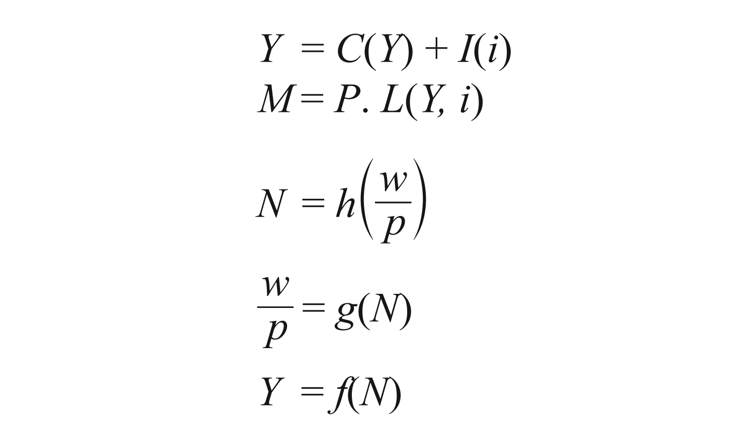
\begin{array}{l} Y = C (Y) + I (i) \\ M = P . L (Y, i) \\ N = h (\frac{w}{p}) \\ \frac{w}{p} = g (N) \\ Y = f (N) \end{array}

(1)

where C, I and L denote consumption, investment and demand for real money balances, respectively. These three variables are, in turn, functions of the endogenous variables. Let the solution to system (1) be (Y¹, P¹, i¹, w¹, N ¹). For later reference, let $\frac{w^{1}}{p^{1}} \equiv {(\frac{w}{p})}^{1}$ .

A brief description of the five equations in system (1) above is as follows. The first equation shows the output level at which the aggregate demand for goods equals the supply of goods. Aggregate demand includes consumption demand and investment demand. The first equation resembles the traditional IS curve, which shows equality between savings and investment (though savings are implicit here as the difference between income and consumption). The second equation shows the equality between supply of and demand for money. This resembles the traditional LM curve. Though the first two equations resemble the IS-LM equations, they are, in fact, different for the simple reason that in the above model P is flexible, which is not the case in the standard IS-LM model.

To complete the description of the model in system (1), the third equation shows that employment in equilibrium is equal to the demand for labour, which is a function of the real wage (w/P). The second last equation says that real wage is equal to the marginal disutility of labour. So, employment is equal to the supply of labour, which depends on the real wage. The last equation shows the standard production function ( f (N) with the properties f ' > 0 and f " < 0).

Money is neutral in this benchmark model but it will be seen in the later variants that this is not the case even where price flexibility is assumed.

As is standard in IS-LM-type models, throughout, it is assumed that the inflation rate is zero (though the model allows for possible changes in the price level in comparative statics exercises). This makes the analysis here comparable to the basic analysis in Keynes (1936) and in related writings.

The conclusion from the benchmark model in this subsection is well known in the literature. Given system (1), the outcome is full employment. This proposition is indeed what Keynes attacked at the beginning of his important book (Keynes, 1936). Given that the outcome in the model is full employment, there is no need for any macroeconomic stabilization by policymakers. However, this conclusion will change in the following subsections.

Market Failure Due to Rigid Prices

The model in the previous subsection has complete price flexibility. This subsection will consider price rigidity. This can take the form of a given price level, a given money wage or a floor on the interest rate. This article will consider the case of money wage rigidity. The case of price level rigidity can be considered somewhat similarly. The treatment of a floor on interest rate is different. This is, however, outside the scope of this article; this author has elsewhere dealt with that case separately.

Let $\bar{w}$ denote the exogenously given money wage. It is assumed that $\bar{w} > w^{1} .$

Recall that w¹ is the equilibrium money wage in system (1). The above inequality is required to allow for unemployment, given the standard Keynesian model with wage rigidity (refer system [2]).

Recall that system (1) had five endogenous variables. Now that the money wage is given, there are four endogenous variables. Accordingly, there is a need to have only four equations so that the system does not become over-determinate. This subsection will drop the second last equation in system (1) which says that the real wage is equal to the marginal disutility of labour (more on this later). The rest of the model is the same as before. So given that $w = \bar{w}$ , the revised model is as follows:

\begin{array}{l} Y = C (Y) + I (i) \\ M = P . L (Y, i) \\ N = h (\frac{\bar{w}}{p}) \\ Y = f (N) \end{array}

(2)

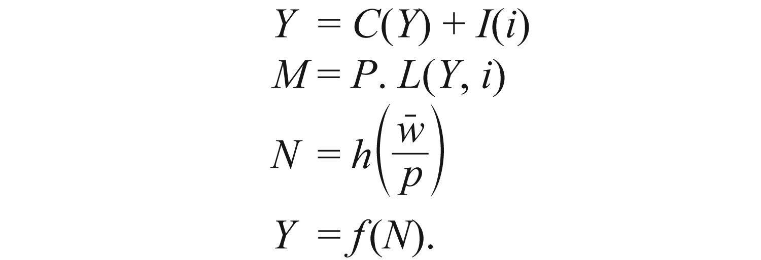
Let the solution to the four endogenous variables in system (2) be (Y ², P ², i ², N ²). Each of these endogenous variables is a function of ( $\bar{w}, M )$ . In this model, less than full employment is possible. In this model,

\frac{\bar{w}}{p^{2}} > g (N^{2}),

where the context for this inequality is the second last equation in system (1); that equation has been replaced by $w = \bar{w}$ in system (2). The inequality means that the real wage is more than the marginal disutility of labour in ‘equilibrium’ (there is a debate on the usage of the term equilibrium in this context in the literature; this issue is, however, outside the scope of this article).

Given the money wage, a policy solution to the problem of unemployment is that the central bank increases money supply. Let the new money supply be M'. Reconsider system (2) with M' instead of M. Let the new solution to the revised version of system (2) be $(Y^{2} (\bar{w}, M^{'}), P^{2} (\bar{w}, M^{'}), i^{2} (\bar{w}, M^{'}), N^{2} (\bar{w}, M^{'})) .$ It is possible to find M' such that

Y^{2} (\bar{w}, M^{'}) = Y^{1},

P^{2} (\bar{w}, M^{'}) = P^{1},

i^{2} (\bar{w}, M^{'}) = i^{1},

N^{2} (\bar{w}, M^{'}) = N^{1} a n d

\frac{\bar{w}}{p^{2} (\bar{w}, ​ M^{'})} = \frac{w^{1}}{p^{1}} .

Recall that be (Y¹, P¹, i¹, w¹, N¹) is the solution to system (1). M' instead of M leads to a vector of prices in equilibrium that are higher so that the prevailing money wage becomes market clearing and it ensures full employment.

To sum up the discussion on, what is sometimes referred to as, the fix-price model in this subsection, unemployment can arise due to money wage rigidity; there is need for government intervention in this model, unlike in, what is sometimes referred to as, the flex-price model in the previous subsection.

This subsection considered wage rigidity. The previous subsection considered price flexibility. Henceforth, unless otherwise specified, the article will return to the assumption that all prices are flexible. Though this assumption was made in the previous subsection as well, there is a difference between the model in the previous subsection and the models in the next two subsections. Also, though there is full employment in the model in the previous subsection, this is not always the case in the following subsections. So it will be seen that though the assumption of price rigidity is sufficient to ensure unemployment, it is not necessary.

Market Failure Due to False Prices

This subsection will reconsider the benchmark classical model in system (1) with flexible prices. However, transitory exogenous disturbances will be incorporated in that model; these now become the source of macroeconomic difficulty.

To see how transitory shocks are incorporated in the benchmark model, consider, for example, the first equation in system (1). Suppose that there is a transitory macroeconomic shock due to, say, a loss of confidence. Consequently, investment falls.⁴ Let us say that the new investment function is J(i) (this is distinct from the normal investment function I(i) as shown in the benchmark system [1]). The new investment function is given by J(i) = I(i) + S₁, where S₁ is a transitory macroeconomic shock. The first equation in system (1) now becomes YCYJiCYIiS₁

This method of incorporating shocks is to retain simplicity in the model. This method can be used more generally to include four other shocks. So, there are, in all, five different transitory shocks included in the model: S₁, S₂, S₃, S₄ and S₅. There is one shock appended to each of the five equations in system (1). Each of the shocks can be positive, zero or negative. So, the model allows for zero value for some shocks, which is the case of absence of a shock.

Recall that system (1) incorporated flexible prices. The revised model with price flexibility and transitory shocks is as follows.

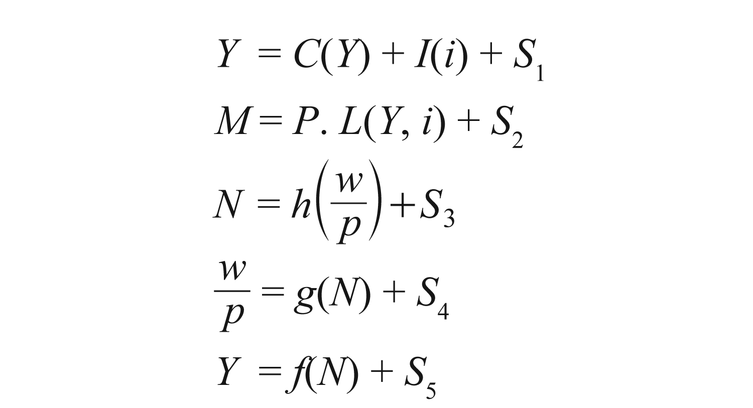
\begin{array}{l} Y = C (Y) + I (i) + S_{1} \\ M = P . L (Y, i) + S_{2} \\ N = h (\frac{w}{p}) + S_{3} \\ \frac{w}{p} = g (N) + S_{4} \\ Y = f (N) + S_{5} \end{array}

(3)

Henceforth, S₁ is interpreted as the transitory macroeconomic shock that affects aggregate demand generally (and not just investment demand) in the first equation in the system. S₂ represents shocks in the money market. Demand for money may shoot up suddenly due to a panic.⁵ S₃ is shock in the context of demand for labour. This article has included this more for the sake of completion than for any other reason. S₄ can represent factors like ‘labour unrest’ which can reduce supply of labour at the prevailing wage rate. (It can even be a change in preference for leisure which reduces the supply of labour; this assumption is sometimes used in the literature on real business cycles.) Finally, S₅ is attached to the production function. It may be identified with a shock that reduces output for a given amount of labour (we may think of a monsoon failure in an emerging economy like India where agriculture and agro-industries are important in one way or another).

There is no uncertainty in the benchmark model (1). To maintain consistency, there is no uncertainty in system (3) as well; it is assumed that the values of the shocks are known in the latter system.

Each of the shocks has a direct effect and an indirect effect. The direct effect works through the equation in which any one shock is included. The indirect effect is due to the system of simultaneous equations.

Let (Y³, P³, i³, w³, N ³) be the solution to system (3). Each of these values is a function of macroeconomic shocks (S₁, S₂, S₃, S₄, S₅).

Let us return to system (1). We will refer to the solution to system (1) as fundamental values of endogenous variables as these are determined by macroeconomic fundamentals and not by any transitory shocks. So (Y¹, P¹, i¹, w¹, N¹) are the fundamental values. On the other hand, the solution to system (3), that is, (Y³, P³, i³, w³, N ³), will be referred to as the set of market values. These incorporate the effects of transitory macro-economic shocks. In the special case in which S_K = 0 ∀k, the market values of variables are the same as the respective fundamental values (refer to system [1]). The usage of the terms fundamental values and market values in the macroeconomic model resembles the usage in the literature on financial markets; in both cases, there can be false prices.

Here the focus is on system (1) and system (3) as both these systems have flexible prices. Here, system (2) is not considered as the latter involves price rigidity. This is not the focus of the article.

Remark 1 on True Prices and False Prices

There are three prices in the model, namely, P, i and w. Let us compare these prices in system (3) with those in system (1). The vector (P¹, i¹, w¹) represents true prices in the sense that these are the outcome of a model that includes fundamentals only. Refer to system (1). In contrast, (P³, i³, w³) are false prices in the sense that these are the outcome of a model that includes macroeconomic shocks even though these are transitory. Refer to system (3).

It is important to stress that though the shocks considered are transitory, they can have considerable effects (in the absence of government intervention). It is also important to reiterate that though transitory shocks have been incorporated in the model, system (3) represents a static model just as system (1) represents a static model. The first result in the article may now be stated.

Proposition 1. Let system (3) represents the economy.

In the general case (transitory shocks S₁, S₂, S₃, S₄, S₅ can take any values), the solution (Y³, P³, i³, w³, N³) is different from (Y¹,P¹,i¹,w¹,N¹).

In the special case in which shocks S₃ = S₄ = S₅ =0 (and S₁, S₂ can take any values), Y ³ = Y ¹, N ³ = N ¹ and ${(\frac{w}{p})}^{3} = {(\frac{w}{p})}^{1}$ . However, the solution (P³, i³, w³) is different from the solution (P¹,i¹,w¹).

Proof: (a) System (1) includes no shocks while system (3) does. Now, the result is obvious. (b) For given values of S ₃, S ₄ and S ₅, the last three equations in system (3) form a self-contained subsystem with only three variables, namely, Y, N and w/P. So these three equations can be solved to get N, Y, and w/P (regardless of the remaining two equations in the entire system). Note that after taking S₃ = S₄ = S₅ = 0, the last three equations in system (3) are the same as the last three equations in system (1). We know that the solution to system (1) has Y¹, N¹ and $(\frac{w^{1}}{p^{1}})$ . So the solution for Y, N and w/P in case of system (3) is the same, given that S₃ = S₄ = S₅= 0. Since N¹ is full employment, it follows that there is full employment in system (3) as well. This is true for all values of S₁ and S₂.

The last three equations in system (3) may be replaced by the following three equations: NN¹YY¹

and

\frac{w}{p} = {(\frac{w}{p})}^{1} .

The first two equations in system (3) remain unchanged. This new system of five equations gives the complete solution. In general, the solutions to the variables i, w and P are not i¹, w¹ and P¹, respectively. The proof is by contradiction. Suppose not. Then i¹, w¹ and P¹ is the solution to system (3) as well. However, comparing system (1) and system (3), we must have S₁ = 0 and S₂ = 0 in system (3). This contradicts the assumption that shocks S₁ and S₂ can take any values. The required result follows.

The model in this subsection included transitory shocks. This subsection examined the effect of the shocks on the endogenous variables. It has been shown that there can be a deviation from full employment due to false prices. In the special case S₃ = S₄ = S₅ = 0, though the solution to the whole system can be different, we have full employment regardless of the values that S₁ and S₂ can take. In the next subsection, we will see that full employment does not prevail even in this special case.

Market Failure Due to False and Abnormal Prices

It has been already seen that price flexibility can lead to false prices. This subsection will now see that price flexibility can have another adverse effect. For this, the notion of the normal price level is introduced. This is the price level that agents in an economy are used to. In this sense, the price level is normal. If there are disturbances and the price level moves away from the normal level, there can be an adverse effect on the real sector in the economy.

The new variant of the model that follows needs to be motivated. For this purpose, there is a need to use a story that is consistent with the model though it is not part of the formal model here. Price flexibility can take the price level⁶ away from its ‘normal’ level. This can lead to a difficulty. The reason is simple. Money is used not just as a medium of exchange but also as a numeraire. Debts are fixed in terms of money. This fixing is after keeping in mind that the price level is at a given level (or the inflation rate is expected to be at a given rate in a model that allows for inflation).

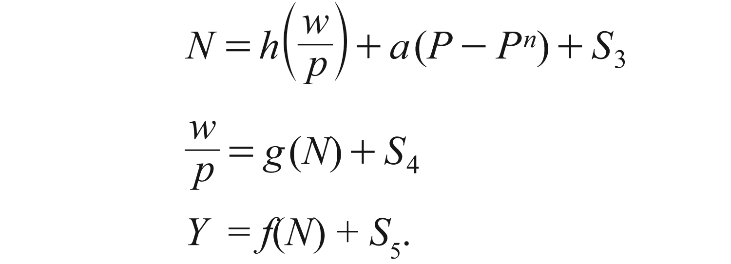
In the debt-deflation theory in Fisher (1933) (and, also in Keynes, 1925), some normal price level matters.⁷ If the actual price level is less than the normal price level, then the real debt of firms rises. This leads to financial stress, and to bankruptcy in extreme cases. So, the supply of output falls. Observe that this is different from the arguments in Keynes (1936), which is a case of fall in demand for output.⁸ In the opposite case where the actual price level is more than the normal price level, firms’ real debt falls. This can make it easier for firms to increase the supply of output. This can, in turn, increase the demand for labour by firms. This response to a gap between the actual price level and the normal price level is captured in the new term included in the demand for labour equation in the model. Refer the third equation in system (4), which includes the new term a(P–Pⁿ), where Pⁿ is the normal price level and a is a constant. The assumption that the new term is included in additive manner is for simplicity only. The rest of system (4) is the same as system (3).

To recapitulate systems with price flexibility in this article, system (1) includes price flexibility. System (3) includes price flexibility and transitory shocks. System (4) includes price flexibility, transitory shocks and effect of possible deviation of the price level from the normal price level. The complete revised model is as follows.

\begin{array}{l} Y = C (Y) + I (i) + S_{1} \\ M = P . L (Y, i) + S_{2} \\ N = h (\frac{w}{p}) + a (P - P^{n}) + S_{3} \\ \frac{w}{p} = g (N) + S_{4} \\ Y = f (N) + S_{5} \end{array}

(4)

If a = 0 in system (4), then the latter system is the same as system (3). The normal price level may be identified with P¹ (see the solution to the variable P in the benchmark system (1) in which shocks are absent). Let (Y⁴, P⁴, i⁴, w⁴, N⁴) denote the solution to system (4). The next result in the article can be stated now.

Proposition 2. Let system (4) represents the economy. Assume that a ≠ 0 and P ⁿ = P¹. The solution to system (4), that is, (Y⁴, P⁴, i⁴, w⁴, N⁴) is different from the solution to system (1), that is, (Y¹, P¹, i¹, w¹, N¹). This is true

in the general case (transitory shocks S ₁ , S ₂ , S ₃ , S ₄ , S ₅ can take any values), and

in the special case in which S₃ = S₄ = S₅ = 0 (and S₁, S₂ can take any values).

Proof: (a) The proof is obvious, given that system (4) includes shocks whereas system (1) does not.

(b) The proposition considers the case a ≠ 0. However, in the hypothetical case of a = 0, it is possible to carve out the last three equations as a separate subsystem in three variables Y, N and $(\frac{w}{p})$ , and solve this subsystem. In the special case S₃ = S₄ = S₅= 0, the subsystem in system (3) is the same as the subsystem of the last three equations in system (1). Accordingly, if and only if a = 0, then Y³ = Y¹, N³ = N¹ and (w/P)³ = (w/P)¹. It is now obvious that if a ≠ 0, the solution to system (4) is different from solution to system (1).

The significance of Proposition 2 is as follows. In the case of system (3) in previous subsection, it was seen that in the special case of S₃ = S₄ = S₅ = 0, there is full employment regardless of the shocks in the first two equations. This is no longer true if the model has system (4). It may be said that false and abnormal prices matter more than just false prices do.

In system (3), false prices are a consequence of transitory shocks. In system (4), false and abnormal prices are a consequence of transitory shocks. Recall that in the special case of S₃ = S₄ = S₅=0, there is full employment in system (3) but possible deviation from full employment in system (4). Refer Proposition 1(b) and Proposition 2(b).

Remark 2 on Price Rigidity as a Policy Target rather than as an Assumption

A deviation from full employment in system (4) is due to the term a(P – Pⁿ) = a(P–P¹) in the third equation; this is with the assumption that Pⁿ = P¹ If somehow policymakers can target and achieve P = P¹, then the effect of the term a (P – Pⁿ) can be avoided and full employment can be attained at least in the case of S₃ = S₄ = S₅. This can explain why Keynes was interested in price level stability as a policy target. In this analysis, there is no assumption of rigidity of the price level (or money wage).

It is true that all this is in the context of the special case S₃ = S₄ = S₅. However, the shocks considered by Keynes involved factors such as loss of confidence and fall in investment demand, or a panic which increases demand for money. These relate to shocks S₁ or S₂ and not to the other three possible shocks included in the model here.

The formal model has so far not considered any government intervention in the economy. The next section will include the policy instruments in the model.

Policy Including the Pigouvian Tax–Subsidy Scheme

It has been seen already that transitory disturbances can lead to a deviation from full employment. Though shocks are transitory in the model, they can last for a while. If there is no policy intervention, then there can be substantial loss to the economy during the period till the shocks go away and till the economy possibly returns to normalcy. In contrast, if there is policy intervention, then the economy can get closer to full employment more quickly and without much adverse effect. Though the time factor is not incorporated in the (static) model here, it is important as a motivation for government intervention.

This subsection will consider policy in the context of the system considered in the previous subsection, namely, system (4). This section will introduce five policy instruments, namely, change in money (ΔM), general government spending (G), taxes on income (T ), (indirect) subsidy/tax on interest cost on investment (z_i) and (indirect) subsidy/tax on labour hired by firms (z_w). The standard policies in macroeconomic models include the first three only, that is, ΔM, G and T. The other two instruments z_i and z_w are not commonly used. The instrument reflected in z_i is used to bring about a change in the market interest rate (i). The instrument reflected in z_i resembles the fiscal instrument used in Jeanne and Korinek (2010b) though the model there is different. The instrument reflected in z_w resembles that discussed informally in Phelps (1994).⁹ The purpose of the new instruments is to correct the false prices in the model (refer to subsection ‘Market Failure Due to False Prices’ for the origin of false prices).

Standard monetary policy here means that the central bank uses the instrument ΔM. Keynesian fiscal policy refers to the use of two instruments (G and T ). Extended fiscal policy means that the government uses Keynesian fiscal policy (G and T ) and ‘new’ fiscal instruments of a tax/subsidy scheme (z_i and z_w).

To provide a perspective on flex-price models in this article, system (1) includes price flexibility. System (3) includes price flexibility and transitory shocks. System (4) includes price flexibility, transitory shocks and effect of possible deviation of the price level from the normal price level. Compared to system (4), system (5) below includes also policy instruments. The complete model is as follows.

\begin{array}{l} Y = C (Y - T) + I (i - z_{i}) + G + S_{1} \\ M + Δ M = P . L (Y, i) + S_{2} \\ N = h (\frac{w - z_{w}}{p}) + a (P - P^{n}) + S_{3} \\ \frac{w}{p} = g (N) + S_{4} \\ Y = f (N) + S_{5} \end{array}

(5)

Compared to system (4), there is an additional component of demand in the economy in the form of government spending (G in the first equation in system [5]). Furthermore, consumption now depends on disposable income (Y – T). Previously, it depended on income (Y). In the second equation, we have M + ΔM in system (5) instead of M in the earlier variants of the model. The first and the third equations in system (4) have been modified to include a subsidy (or tax) on interest cost on investment, and a subsidy (or tax) on labour cost for firms.¹⁰

Note that i appears in the system twice—in the first equation and in the second equation. However, the instrument z_i is used in the first equation only. The reason is that the tax/subsidy applies to the interest cost on investment (in the real sector). It does not apply to interest rate per se in the financial/money market. It may be said that the policy to affect interest rate for varying investment demand is better targeted in this new model compared to what is done in the standard Keynesian model.

Let (Y⁵, P⁵, i⁵, w⁵, N⁵) denote the solution to system (5), given the policy instruments ΔM, G, T, z_i and z_w (and also shocks S₁, S₂, S₃, S₄, S₅).

The public authorities need to choose the optimal values of its instruments.¹¹ The objective is to reduce the deviation of X⁵ from X¹, where X ϵ {Y, P, i, w, N}. Let _p, _i, _w and _N denote the weights policymakers attach to minimization of square of deviations from optimal values (P⁵ – P¹)², (i⁵ – i¹)², (w⁵ – w¹)² and (N⁵ – N¹)², respectively. (The weight attached to (Y⁵ – Y¹)² is normalized at 1.) Consider now the following optimization exercise on the part of the policymakers.

Programme 1. Minimize

\begin{matrix} £ = {(Y^{5} - Y^{1})}^{2} + α_{p} {(P^{5} - P^{1})}^{2} + α_{i} {(i^{5} - i^{1})}^{2} + \\ α_{w} {(w^{5} - w^{1})}^{2} + α_{N} {(N^{5} - N^{1})}^{2} \end{matrix}

with respect to MGTz_iz_w

Recall that (Y⁵, P⁵, i⁵, w⁵, N⁵) are functions of the policy instruments ΔM, G, T, z_i and z_w. Denote these optimal values by $(Δ M^{*}, G^{*}, T^{*}, z_{i}^{*}, z_{w}^{*}) .$

The special case of Programme 1 is when _i = _w = _N = 0. This is the case which is more familiar in the macroeconomic literature. Here, the model will consider the general case.

The next result in this article is as follows:

Proposition 3. Given system (5), a ! 0 and Pⁿ = P¹,

policymakers cannot ensure the outcome (Y ¹ , P ¹ , i ¹ , w ¹ , N ¹ ), and

policymakers can ensure the outcome $X^{5} (Δ M^{*}, G^{*}, T^{*}, z_{i}^{*}, z_{w}^{*}) .$ where X d {Y, P, i, w, N}.

Proof: (a) The first part of the proposition is proved by contradiction. Suppose not. Then, (Y¹, P¹, i¹, w¹, N¹) satisfies system (5) for some values of ΔM, G, T, z_i and z_w. In particular, (P¹, w¹, N¹) will satisfy the fourth equation. But this implies that S₄ = 0 since (Y¹, P¹, i¹, w¹, N¹) is the solution to system (1) (refer the fourth equation in system [1]). However, S₄ = 0 contradicts the assumption that S₄ can take any value. This completes the proof.

(b) The proof is obvious.

Let us turn next to a corollary that follows from Proposition 3.

Corollary 1: The policy package that includes extended fiscal policy and standard monetary policy is more effective than the policy package that includes Keynesian fiscal policy and standard monetary policy.

Proof: In case of extended fiscal policy and standard monetary policy, ΔM, G, T, z_i and z_w can take any value in Programme 1. In contrast, in case of Keynesian fiscal policy and standard monetary policy, ΔM, G and T can take any value but z_i = z_w = 0. The result is now obvious.

Before the article is concluded, it is important to make some informal comments on the sustainability of extended fiscal policy. At present, the public authorities are expected to use Keynesian fiscal policy and the standard monetary policy to overcome a recession. Observe that this has two features. First, fiscal policy includes Keynesian fiscal policy only; it does not include the Pigouvian tax–subsidy scheme to correct false prices. Second, though it may have been thought that the stabilization policy will be used in both a recession and a boom, there is a much stronger requirement in practice in case of a recession only; there is hardly any compelling provision in case of a boom in practice. The result is that there are deficits in recessions but hardly any surpluses in booms. So, there is typically accumulation of debts incurred in recessions. In view of this, there is a need to make two changes. First, the fiscal policy for macroeconomic stabilization needs to include not only the Keynesian fiscal policy but also the Pigouvian tax–subsidy scheme. Observe that this is not a subsidy scheme or a tax scheme; it is instead a tax–subsidy scheme. So there can be a tax in one case and a subsidy in another case. This can help with keeping any imbalance in the budget for macroeconomic stabilization to the minimum. Second, it needs to be made mandatory that the policy for stabilization is used in not only a recession but also in a boom (though of course the policy needs to be used differently in the two cases). For this purpose, it is important to have the changes in the form of amendments to the constitution to ensure a commitment to policy in not only a recession but also in a boom.

The proposed tax–subsidy scheme can lead to an administrative burden for the tax department of the government. However, a close look shows that this apprehension is not very valid. Note that firms file tax returns anyway. Under the proposed policy, firms just need to include subsidy claims or tax obligations related to the tax–subsidy scheme proposed in the article. Furthermore, observe that the fixed cost of administration involved in tax returns is incurred anyway. It is only the variable cost which can go up. But in these days of information technology, these variable costs can be low and they can be falling over time (with technological improvements and increasing effective competition). So the administrative cost does not appear to be a major issue. More specifically, it is a matter of revising the software that is used for accounting and taxation purposes; the software includes the software used by firms and that used by the tax department. Thereafter, routine keeping of records and filing of returns takes care of the additional features proposed here.

In the model, the treasury can provide a subsidy in recession and can impose a tax in a boom. It may appear that there is hardly any net gain to firms inter-temporally. However, the value of a subsidy received in a recession can be more than the pain of a tax in a boom; this is because it is much harder to get funds in a recession than in a boom. So the Ricardian equivalence does not hold. Accordingly, the policy proposed in the article is effective. Also, if the subsidy on investment in a recession acts as a signal of good times that could be coming and that can raise the expectation of output and other such variables in the future, then Ricardian equivalence does not hold a fortiori and the proposed policy can be even more effective than it would be otherwise.

The comments here are confined to government budget as it relates to macroeconomic stabilization. It is true that in practice many more issues related to development economics and political economy are involved. These are important but these are outside the scope of this article.

Conclusion

The standard Keynesian models (including the New Keynesian model) assume that prices are rigid. However, it is interesting that Keynes himself did not make such an assumption and yet he argued that less than full employment can be an outcome in equilibrium. Following Keynes and other authors such as Leijonhufvud, Patinkin and Farmer, this article does not assume any price rigidity. So this is not the source of the macroeconomic problems in our model. The problem in our model lies elsewhere. There can be transitory macroeconomic shocks and these can lead to false prices and to abnormal prices. These can play a role in the deviation of output from its full employment level.

The conventional wisdom is that price flexibility can be useful in economics, which is indeed the case. However, price flexibility can at times play a negative role. It can accommodate effects of macroeconomic shocks even when these are transitory. It can also take the price level (or the exchange rate) away from the normal levels. Consequently, there can be adverse effects on output and employment. These novel elements (or their implications) were integrated in a very simple model in this article.

On the policy side, it was shown that a tax–subsidy scheme can be used to neutralize transitory shocks that affect prices, which are important in macroeconomics. Such a tax–subsidy scheme can be used alongside the standard Keynesian fiscal policy. There can be an optimal mix of the two different fiscal policies. This article referred to such a set of fiscal policies as the extended fiscal policy.

This article considered two (relative) prices, namely, interest rate and wage rate, which are important in macroeconomics as applied to a closed economy. The tax–subsidy scheme was considered as a corrective measure in the context of these two prices. However, the basic argument applies more generally and it can be applied to other prices that may be included in an open economy model or a more elaborate closed economy model.

The model in this article has incorporated transitory shocks, and Pigouvian type tax-subsidy scheme that can somewhat correct or neutralize the effects of transitory shocks. In doing so, the article has made the market failure in macroeconomics methodologically close to the market failure in public economics.

Footnotes

Acknowledgements

I thank Partha Sen for his valuable comments on the initial draft of the article. I also thank E. Somanathan for his feedback on the section on transitory macroeconomic disturbances and Pigouvian-type tax–subsidy scheme. The complete article was presented at the 9th Annual Conference on Economic Growth and Development, December 2014 at ISI, Delhi Centre. I thank the organizers and the seminar participants. The article in its current form is a thoroughly revised version of the earlier drafts. Last but not the least, I thank an anonymous referee for making some very useful suggestions on improving the article. Any errors are my responsibility.

Notes

References

Bernanke

, & Gertler

(1989). Agency costs, net worth, and business fluctuations. The American Economic Review, 79(1), 14–31.

Blinder

A. S.

(2013). After the music stopped—The financial crisis, the response, and the work ahead. New York, NY: Penguin.

Buiter

(2009, March 03). The unfortunate uselessness of most ‘state of the art’ academic monetary economics. Financial Times. Retrieved 23 July 2010, from ft.com/maverecon.

Caballero

R. J.

(2010). Macroeconomics after the crisis: Time to deal with the pretense-of-knowledge syndrome. Journal of Economic Perspectives, 24(4), 85–102.

De Long

J. B.

, & Summers

(1986). Is increased price flexibility stabilizing? The American Economic Review, 76(5), 1031–1044.

Dimand

R. W.

(2008). Macroeconomics, origins and history of. In Durlauf

S. N.

& Blume

L. E.

(Eds), The new Palgrave dictionary of economics (2nd ed., Vol. 5, pp. 236–244). New York, NY: Palgrave Macmillan.

Fair

R. C.

(2012). Has Macro progressed? Journal of Macroeconomics, 34(1), 2–10.

Farmer

(2010). Expectations, employment and prices. New York, NY: Oxford University Press.

Fisher

(1933). The debt deflation theory of great depressions. Econometrica, 1(4), 337–357.

10.

Friedman

(1988, April 15). The fed has no clothes. The Wall Street Journal.

11.

Friedman

, & Schwartz

A. J.

(1963). A monetary history of the United States, 1867–1960. Princeton, NJ: Princeton University Press.

12.

Gopinath

, & Itskhoki

(2011). In search of real rigidities. NBER Macroeconomics Annual 2010, 25, 261–310.

13.

Jeanne

, & Korinek

(2010a). Excessive volatility in capital flows: A Pigouvian taxation approach. The American Economic Review: Papers & Proceedings, 100(2), 403–407.

14.

Jeanne

, & Korinek

(2010b). Managing credit booms and busts: A Pigouvian taxation approach (NBER Working Paper, w16377). Cambridge, MA: National Bureau of Economic Research.

15.

Keynes

J. M.

(1925). The economic consequences of Mr. Churchill. London: L. and V. Woolf.

16.

Keynes

J. M.

(1936). The general theory of employment, interest, and money. London: Macmillan.

17.

Leijonhufvud

(1981). Information and coordination: Essays in macro-economic theory. New York, NY: Oxford University Press.

18.

Lucas

R. E.

Jr. (1972). Expectations and the neutrality of money. Journal of Economic Theory, 4 (April), 103–124.

19.

Mankiw

N. G.

(2006). The macroeconomist as scientist and engineer. The Journal of Economic Perspectives, 20(4), 29–46.

20.

Mian

, & Sufi

(2014). House of debt—how they (and you) caused the Great Recession, and how we can prevent it from happening again. Chicago, IL: University of Chicago Press.

21.

Minsky

(1978). The financial instability hypothesis—A restatement. Hyman P. Minsky Archive, 180. Retrieved from http://digitalcommons.bard.edu/hm_archive/180

22.

Mishkin

F. S.

(2004). The economics of money, banking, and financial markets (7th ed., Series in Economics). Boston, MA: The Addison-Wesley.

23.

Palley

T. I.

(2004). Asset-based reserve requirements: Reasserting domestic monetary control in an era of financial innovation and instability. Review of Political Economy, 16(1), 43–58.

24.

Patinkin

(2008). Keynes, John Maynard. In Durlauf

S. N.

& Blume

L. E.

(Eds), The New Palgrave Dictionary of Economics (2nd ed., Vol. 4, pp. 687–716). New York, NY: Palgrave Macmillan.

25.

Phelps

E. S.

(1994). Low-wage employment subsidies versus the welfare state. The American Economic Review, 84(2), 54–58.

26.

Romer

(2012, January). Short-run fluctuations. University of California, Berkeley. Retrieved from https://eml.berkeley.edu//~dromer/papers/Romer%20Short-Run%20Fluctuations%20January%202012.pdf

27.

Selgin

, Lastrapes

W. D.

, & White

L. H.

(2012). Has the FED been a failure? Journal of Macroeconomics, 34(3), 569–596.

28.

Solow

(2010). Building a science of economics for the real world. Prepared statement to the House Committee on Science and Technology, Subcommittee on Investigations and Oversight, July 20, 2010.

29.

The Economist (2016, January 10). Flexible figures. Retrieved 3 March 2018, from https://www.economist.com/news/business/21689541-growing-number-companies-are-using-dynamic-pricing-flexible-figures

30.

Tinbergen

(1955). On the theory of economic policy (2nd ed.). Amsterdam: North-Holland Publishing Company.

31.

Woodford

(2009). Convergence in macroeconomics: Elements of the new synthesis. American Economic Journal: Macroeconomics, 1(1), 267–279.