Gravity Models in International Trade: An Exploration in Econo-Physics

Abstract

Several strands of the static and dynamic theoretical constructs and the empirical applications in the subject of economics owe substantially to the well-known principles of physical sciences. The present article explores as to how the development of the popular gravity models in international trade can be traced back to Newton’s law of gravitation, and to both Ohm’s Law and Kirchhoff’s Law of current electricity, as well as to the pattern recognition techniques commonly deployed in scientific applications. In addition to surveying these theoretical analogies, the article also offers numerical applications for observed trade patterns between India and a set of countries.

JEL Classifications: F41, F42, C61, F47

Keywords

International trade gravity models Ohm’s Law cross-country India

Introduction

The general laws of economics and subsequently, numerous ramifications of the subject that offer firm bases for neoclassical and post-Keynesian analytical dimensions borrow copiously from the physical sciences. The present article offers a brief review of the commonalities between the Gravity Model used abundantly in the subject of international trade for multiple countries and those of the fundamental laws in physics. Since, the adaptation of the laws of physics into mainstream economics is both common and proven efficient, a number of compelling relations have found great acceptances and widespread applications. In the same vein, in 1954, Walter Isard was inspired by Newton’s law of gravitation and developed an analytical framework for the study of international trade between countries—one that is different from the celebrated Heckscher–Ohlin predictions about the patterns of trade along a much-less traversed territory in economics, namely, networks. The core idea, which requires little explanation, is based on the standard gravitational relation akin to the planetary motions and classifications according to the hub-and-spoke formations between countries. However, subsequently, Tinbergen (1962), Poyhonen (1963), and Linneman (1966) independently proposed analytical frameworks for the study of international trade similarly inspired by Newton’s law of gravity. The present structure of the Gravity Model is a mixture of these constructs with a number of additional attributes and factors since accommodated in order to lend better predictive abilities to the core model. In its more recent avatars, the model has found strong applications in the works of Anderson (1979), Bergstrand (1985), Markusen (1986), Helpman (1987), Bergstrand (1989), Dhar and Panagariya (1994), Davies (1995), Eaton and Kortum (1997), Deardorff (1998), Evenett and Keller (1998), Feenstra et al. (1999) as well as Anderson and Wincoop (2003, 2004), Baldwin and Taglioni (2006), Chaney (2008), etc. Note that, these constitute essentially theoretical reconstructions of the basic model and are obviously accompanied by a large number of country-studies, which do not automatically enter the present survey unless we take recourse to certain examples where the patterns of bilateral and multilateral trade display deeper connections with one or more laws of physics.

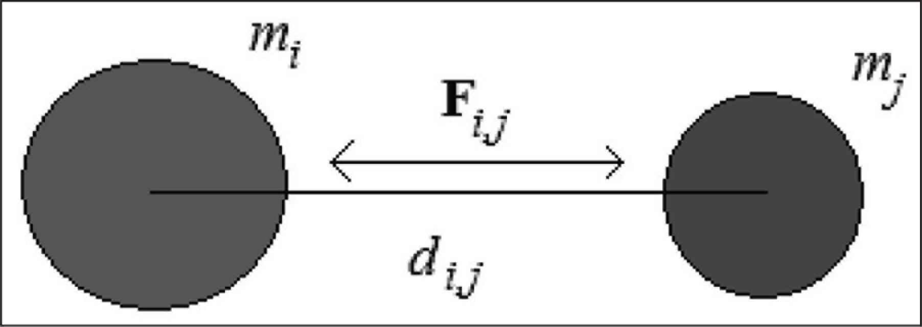
Indeed, in 1686 when Sir Isaac Newton postulated the law of universal gravitation in classical mechanics of physics, little was imagined that the prevailing mercantilist trade patterns soon-to-become instruments of pervasive colonial expansions, were intrinsically governed by the law of gravity also. This law, however, measures the force of attraction between two different bodies placed at a particular distance, as shown in Figure 1.

In order to define the scope and perspective of this research, let us reiterate Newton’s law of universal gravitation as follows: every particle attracts every other particle in the universe with a force which is directly proportional to the product of their masses and inversely proportional to the square of the distance between their centres. However, before we lay out the details of how Newton’s Law influences the gravity model in clearer terms, it might be useful to discuss the broad connections at the outset.

Figure 1.

Source: The authors.

It follows from the seminal work of Tinbergen (1962) that the size of bilateral trade flows between any two countries can be approximated by a law called the gravity equation, which as mentioned above is a derivative of the Newtonian theory of gravitation. Just as planets are mutually attracted in proportion to their sizes and proximity, countries trade in proportion to their respective GDPs and proximity (also see, Yotov et al., 2016). It is well-known that the gravity model in trade was initially considered merely as an empirical observation with little theoretical basis. Empirically speaking, the stable relationship between the size of trading economies, their distance and the amount of trade explained the creation and sustenance of networks successfully, but these did not seem to subscribe to the fundamental theorems of international trade relying heavily on the Ricardian structure highlighting differences in technology across countries to explain trade patterns, and the Heckscher–Ohlin model holding differences in factor endowments among countries as the basis for trade. It was believed that gravity equations introduced factors that were either (indirectly) subsumed under the explanations available in the classical models; or that the factors were too esoteric to have wider applicability. For example, country size has little to do with the structure of trade flows in classical models. Regardless, the extraordinary stability of the gravity equation and its power to explain bilateral trade flows prompted the search for a theoretical explanation for it. With regard to gravity models while empirical analysis predated theory, it presently appears that most trade models require gravity in order to work. In this connection, later modification to the trade theory a’la Krugman (1980) is more amenable to the empirical observations from the gravity model. In fact, Bergstrand (1985, 1989) also shows that a gravity model reflects trade due to monopolistic competition in the product market and that a preference for variety between identical countries influences the network formation. It argues that the presence of monopolistic competition and taste for variety within similar countries overcome the undesirable features of Armington models where goods are differentiated only by location of production. Consequently, firm location is endogenous rather than based on restrictive assumptions in other models and all trading countries could specialize in the production of different sets of goods. Notwithstanding, Deardorff (1998) showed that a gravity model can arise from differences in factor-proportions as part of traditional explanations. Further, Eaton and Kortum (2004) derived a gravity-type equation from a Ricardian model, while Helpman et al. (2008) and Chaney (2008) related the structure of gravity equations to models with differentiated goods and heterogeneous firms.

In conformity with the law of gravity, the gravity models in trade expects volume of trade to be positively affected by GDP (the economic mass) and negatively related to the distance - a pattern of trade that would not be directly predictable by the Heckscher–Ohlin model, unless of course, the importance of distance and trade costs proportional to it (Iceberg costs as in Dornbusch–Fischer–Samuelson, 1977) as extensions of the Ricardian structure are factored in. The success of the gravity model in empirical international economics may therefore be explained by the fact that it yields results that justify inclusion of non-trivial factors like distance between countries and trade costs as opposed to the frictionless world in Hekscher–Ohlin models and realistically predict the volume and direction of trade between countries. Notwithstanding, high trade costs may also be considered as a fixed ‘entry’ cost and the consequent trade pattern might collapse to Hekscher–Ohlin predictions if such costs are not compensated by large markets at destinations (see Marimoutou et al., 2010).

Given this background, the rest of the survey article is organized as follows. The next section discusses Newton’s Law in relation to the economic implications of the gravity model. The third section deals with the parametric specifications of the gravity equations, especially, distance, cost of transportation, common borders, trade barriers and agreements, climate, religion, etc. The fourth section deals with the question of remoteness and nearness between countries and offers indices that can ideally be part of the estimates based on gravity models. In this section we also invoke analogy with other applied models of physics, namely the electric circuits serving as networks. The fifth section discusses a unified gravity model, and the sixth section concludesthe article.

Newton’s Law of Gravitation in Economics

This law is mathematically described as follows.

Let

m_i = mass of a particle or body i,

m_j = mass of another particle or body j,

d_i,j = distance between the particle or body i with mass m_i and the particle or bodyj with mass m_j

(Note: The distance is measured between the centres of them)

F_i,j = force of attraction between the particle or body with mass m_i and the particle or body with mass m_j, and

G = a constant, known as Gravitational constant.

Then the model can be described mathematically, as

F_{i, j} \propto m_{i} m_{j},

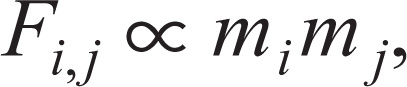
when d_i,j remains unchanged, and

F_{i, j} \propto \frac{1}{d_{i, j}^{2}},

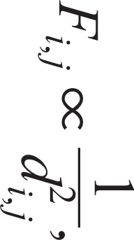
when m_i and m_j remain unchanged.

Now by joint variation

F_{i, j} \propto \frac{m_{i} \times m_{j}}{d_{i, j}^{2}},

(1)

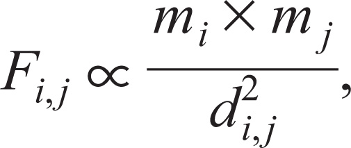
when m_i, m_j and d_i,j are variables.

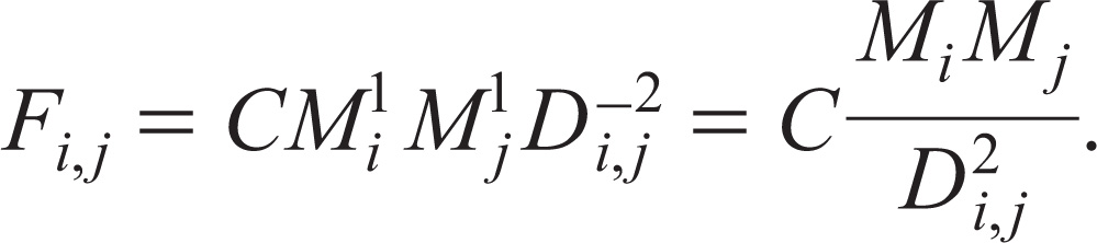
Therefore, the Newton’s law of gravitation is mathematically described by Equation (2).

F_{i, j} = G \frac{m_{i} \times m_{j}}{d_{i, j}^{2}},

(2)

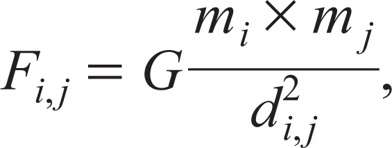
where, G = a constant, known as Gravitational constant.

Illustration 1. Suppose masses of two bodies are 5.5 × 10⁸ kg and 2.3 × 10¹⁵ kg respectively. They are separated by a distance 2000 m. Compute the force of attraction between the bodies. Assume Gravitational constant $G = 6.67 \times \frac{10^{- 11} N m^{2}}{k g^{2}}$ (where kg= kilogram, m=metre, N= newton are the units of measurement).

Here,

\begin{array}{l} m_{i} = 5.5 \times 10^{8} k g, \\ m_{j} = 2.3 \times 10^{15} k g, \\ d_{i j} = 2000 m a n d \\ G = 6.67 \times \frac{10^{- 11} N m^{2}}{k g^{2}} . \end{array}

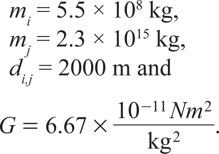
Then the force of attraction between m_i and m_j placed at distance d_i,j is

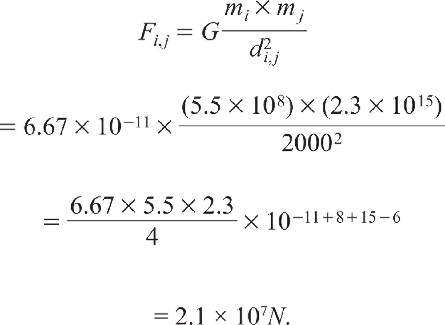
\begin{matrix} F_{i, j} = G \frac{m_{i} \times m_{j}}{d_{i, j}^{2}} \\ = 6.67 \times 10^{- 11} \times \frac{(5.5 \times 10^{8}) \times (2.3 \times 10^{15})}{2000^{2}} \\ = \frac{6.67 \times 5.5 \times 2.3}{4} \times 10^{- 11 + 8 + 15 - 6} \\ = 2.1 \times 10^{7} N . \end{matrix}

Ñ Force of attraction is 2.1 × 10⁷ N.

Analogy of Gravitation in Economics

Newton’s law of gravitation can be viewed in economics as follows.

Let

m_i = Economic mass for country i,

m_j = Economic mass for country j,

D_i,j = Geographical distance between country i and country j,

F_i,j = Force of trade flow between country i and country j.

Assume M_i and M_j are described in the same scale or unit.

The following hypothesis are the basis of international trade

Larger countries trade more than smaller ones, that means trade depends on the economic mass of the country, and

Geographical distance between two trade partners (i.e., countries) reduces trade force between them.

Intuitive Idea of Gravity Model in Economics

Newton’s law of gravitation is the inspiration for the design of an intuitive gravity model for trade.

The trade force depends on the economic mass of the countries. This says that the trade force is directly proportional to the economic mass of the countries.

Mathematically,

F_{i, j} \propto M_{i} M_{j},

when D_i,j remains unchanged.

Geographical distances between two trade partners (i.e., countries) reduce trade force between them. This says that the trade force is inversely proportional to the geographical distance between partner countries.

Mathematically,

F_{i, j} \propto \frac{1}{D_{i, j}^{2}},

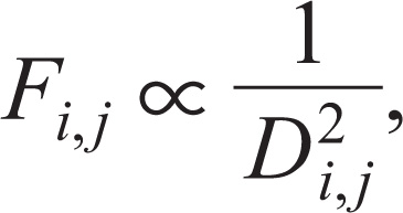
when M_i and M_j remain unchanged.

These may be combined and described as in Equation (3).

F_{i, j} = C \frac{M_{i} M_{j}}{D_{i, j}^{2}},

(3)

where, C = Constant of variations.

Here, we can assume that economic mass means, GDP (or export or import) of the country and distance means physical distance between two partner countries for trade. Intuitively export (or trade) between two countries depend on their economic masses and negatively related to the distance between them.

Illustration 2. In 1996 the GDP of India was $3.83 × 10¹¹ and the GDP of Australia was $4.01 × 10¹¹. The geographical distance between India and Australia is 10363.85 Km. Compute the trade force of attraction between the countries India and Australia. Assume constant C = 1

This is shown in Figure 2.

Here,

m_India = Economic mass, that is, GDP of India = $3.83 × 10¹¹,

m_Australia = Economic mass, that is, GDP of Australia = $4.01 × 10¹¹,

D_{India,Australia}

= Geographical distance between India, and Australia

= 10363.85 Km, and

C = 1.

Then, the trade force of attraction between India and Australia is

\begin{array}{l} F_{I n d i a, A u s t r a l i a} = C \times \frac{M_{I n d i a} \times M_{A u s t r a l i a}}{D_{I n d i a, A u s t r a l i a}^{2}} \\ \begin{array}{l} = 1 \times \frac{(3.83 \times 10^{11}) \times (4.01 \times 10^{11})}{{(10363.85)}^{2}} \\ = 1.43 \times 10^{15} . \end{array} \end{array}

Figure 2.

Source: www.printablee.com

Ñ Trade force of attraction is 1.43 × 10¹⁵ unit.

Gravity Model in International Trade

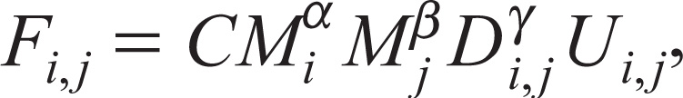
In Newton’s law of gravitation, Newton postulated and described mathematically that it strictly follows the rule defined in Equation (1) in case of earth science. But in case of international economics, the trade flow apparently follow the rule defined in Equation (3). It varies from case to case, in this context we define a generalized model for Equation (3) in Equation (6).

F_{i, j} = C M_{i}^{α} M_{j}^{β} D_{i, j}^{γ},

(4)

where,

m_i = Economic mass for country i,

m_j = Economic mass for country j,

D_i,j = Geographical distance between country i and country j,

F_i,j = Force of trade flow between country i and country j

α, β, γ = parameters of the model.

If we assume α, β are positive and γ is negative, then Equation (6) is a generalized version of Law of Gravity defined in Equation (2).

Illustration 3. If we choose α = 1, β = 1 and γ = –2 then Equation (6) can be written as

F_{i, j} = C M_{i}^{1} M_{j}^{1} D_{i, j}^{- 2} = C \frac{M_{i} M_{j}}{D_{i, j}^{2}} .

(5)

This is equivalent to Newton’s law of gravitation.

Empirical Gravity Model in Econometrics

An empirical gravity model is design based on the relation (6).

Now we introduce a random fluctuation U_i,j with Equation (6), then we can write as follows:

F_{i, j} = C M_{i}^{α} M_{j}^{β} D_{i, j}^{γ} U_{i, j},

(6)

when the expected value of U_i,j, that is, E(U_i,j) = 1.

By taking ‘ ln ’ that is, ’log’ operator on both sides of Equation (6), we get

\ln F_{i, j} = \ln C + α \ln M_{i} + β \ln M_{j} + γ \ln D_{i, j} + \ln U_{i, j} .

(7)

Therefore, an empirical equation for basic gravity model is described by relation (8) which is almost similar to Equation (7).

\ln X_{i, j} = b_{0} + b_{1} \ln Y_{i} + b_{2} \ln Y_{j} + b_{3} \ln D_{i, j} + e_{i, j},

(8)

where,

Y_i = Economic mass for country i,

Y_j = Economic mass for country j,

D_i,j = Distance between country i and country j,

X_i,j = Force of trade flow between country i and country j

e_i,j = Random error term when trade flow between country i and country j, that is, e_i,j:N(0,σ), that is, normal distribution with standard deviation σ and mean 0,

E(e_i,j) = expected value of e_i,j

= 0

b₀, b₁, = Parameters of the model.

b₂, b₃

Note that conditions b₁, b₂ > 0; b₃ < 0 says that it is similar to gravity model.

Constituents of the Gravity Model

The gravity models have a number of features that make it quite distinct.

The gravity model yields good results in explaining bilateral flows; and more fundamentally,

The gravity model helps identifying countries that would realistically engage in trade—a prediction that Heckscher–Ohlin model leaves unspecified (Marimoutou et al., 2010).

In addition,

The mass variables, such as, GDP, exports or imports, can be easily accommodated in the gravity model (Feenstra et al., 1999).

Since, geographical distance, as an indicator could approximate the cost of entry in a market (e.g., the greater the distance, the higher the entry cost) in a gravity model (see Egger, 2008).

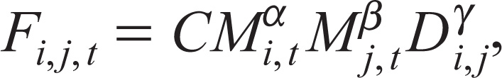
The geographical distance D_i,j between country i and country j is a fixed quantity in the gravity model, but the economic mass of a country changes with time t. So it is necessary to introduce the time variable t with the gravity model. In this context Equation (6) can be rewritten as Equation (9).

F_{i, j, t} = C M_{i, t}^{α} M_{j, t}^{β} D_{i, j}^{γ},

(9)

where,

M_i,t = Economic mass for country i at time t,

M_j,t = Economic mass for country j at time t,

D_i,j = Geographical distance between country i and country j,

(Note: this variable does not change with time t)

F_i,j,t = Force of trade flow between country i and country j at time t

α, β, γ = Parameters of the model.

Similarly, Equation (8) can be rewritten as Equation (10).

\ln X_{i, j, t} = b_{0} + b_{1} \ln Y_{i, t} + b_{2} \ln Y_{j, t} + b_{3} \ln D_{i, j} + e_{i, j},

(10)

where,

Y_i,t = Economic mass for country i at time t,

Y_j,t = Economic mass for country j at time t,

D_i,j = Distance between country i and country j,

X_i,j,t = Force of trade flow between country i and country j at time t,

e_i,j = Random error term when trade flow between country i and country j

E(e_i,j) = expected value of e_i,j

= 0

b₀, b₁, = Parameters of the model in which b₃ < 0

b₂, b₃ since ‘distance is negatively proportional to the trade force’.

At this point, further explanations about including distance as an indicator is given below.

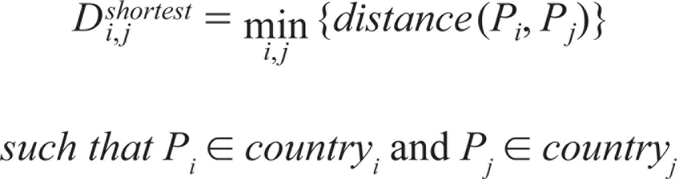
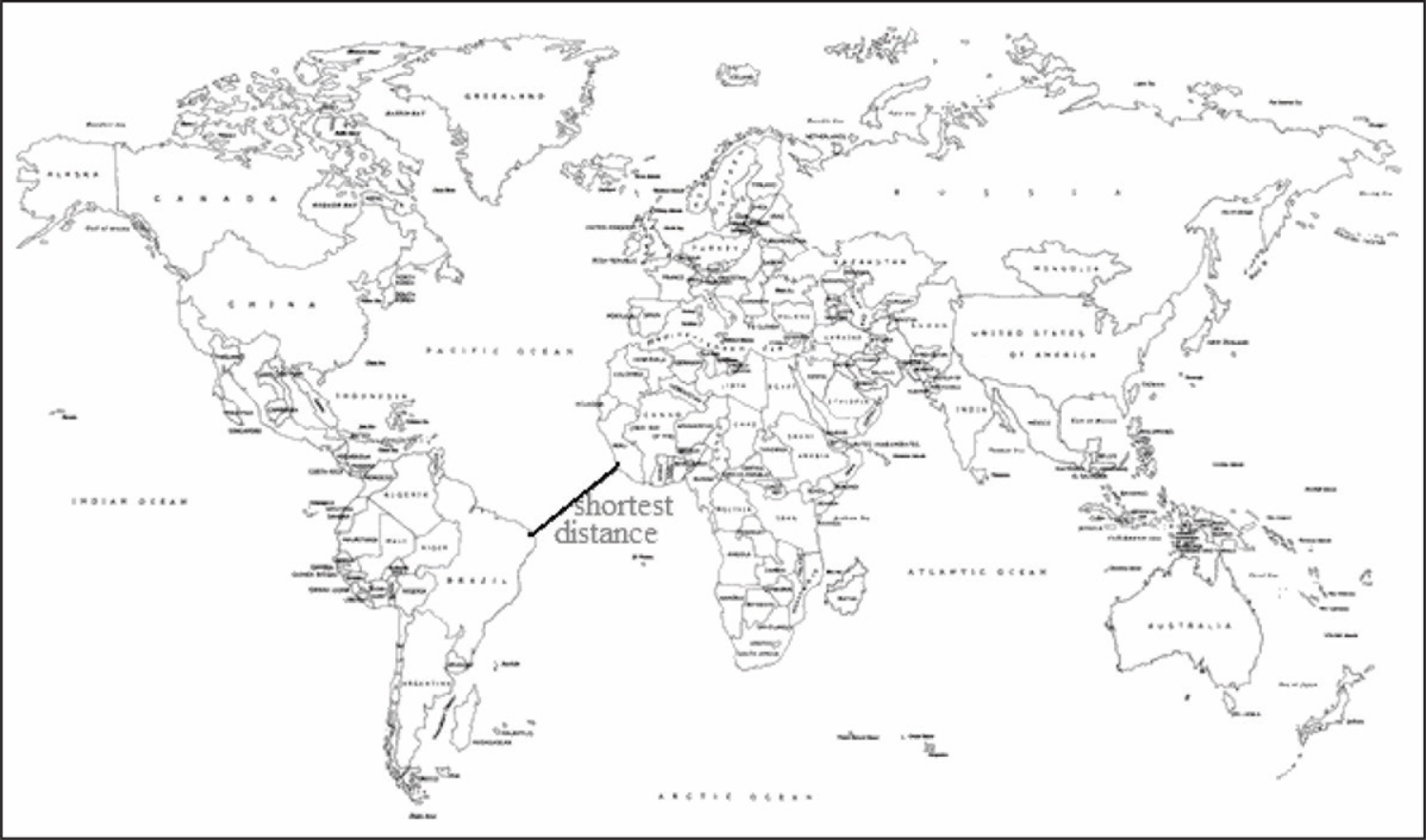
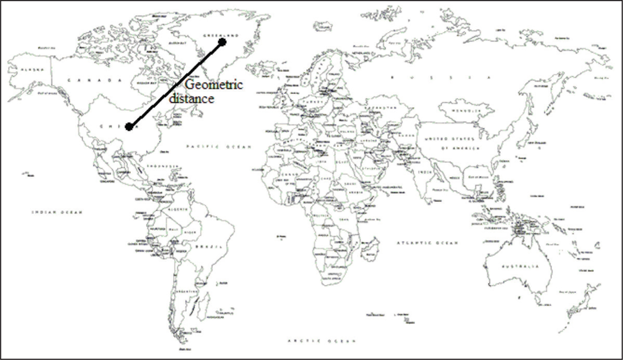
Shortest distance between two countries: It is the minimum distance, $D_{i, j}^{s h o r t e s t}$ , between two points P_i and P_j where P_i ∈ country i and P_j ∈ country j, that is,

\begin{array}{l} D_{i, j}^{s h o r t e s t} = \min_{i, j} {d i s ​ \tan ​ c e (P_{i}, P_{j})} \\ s u c h t h a t P_{i} \in c o u n t r y_{i} a n d P_{j} \in c o u n t r y_{j} \end{array}

Note that $D_{i, j}^{s h o r t e s t} = 0$ , when country i and country j are adjacent countries, and they have common borders.

Illustration 4. Shortest distance between two countries X and Y is shown in Figure 3.

Geometric distance between two countries: It is the distance, $D_{i, j}^{g e o m e t r i c}$ , between two points P_i and P_j in a straight line,

where,

P_i = centre of the area of country i,

P_j = centre of the area of country j.

Figure 3.

Source: www.printablee.com

Illustration 5. Geometric distance between two countries X and Y is shown in Figure 4.

Aerial distance between two countries: It is the distance, $D_{i, j}^{a i r}$ , between two points P_i and P_j in a straight line,

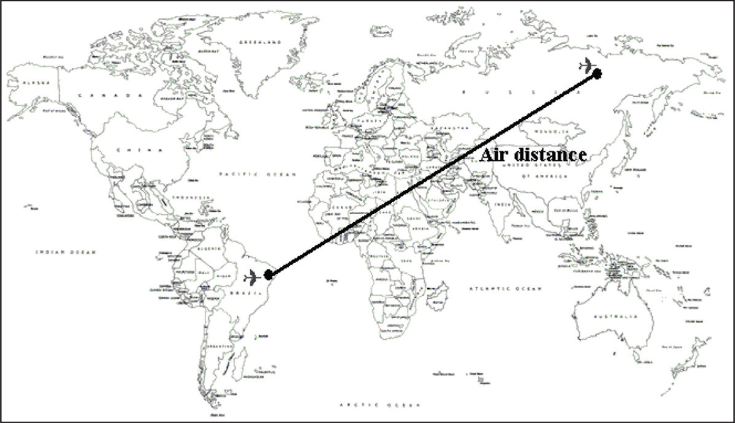
where,

P_i = an airport (e.g., source/ destination) of the country i,

P_j = an airport (e.g., destination/ source) of the country j.

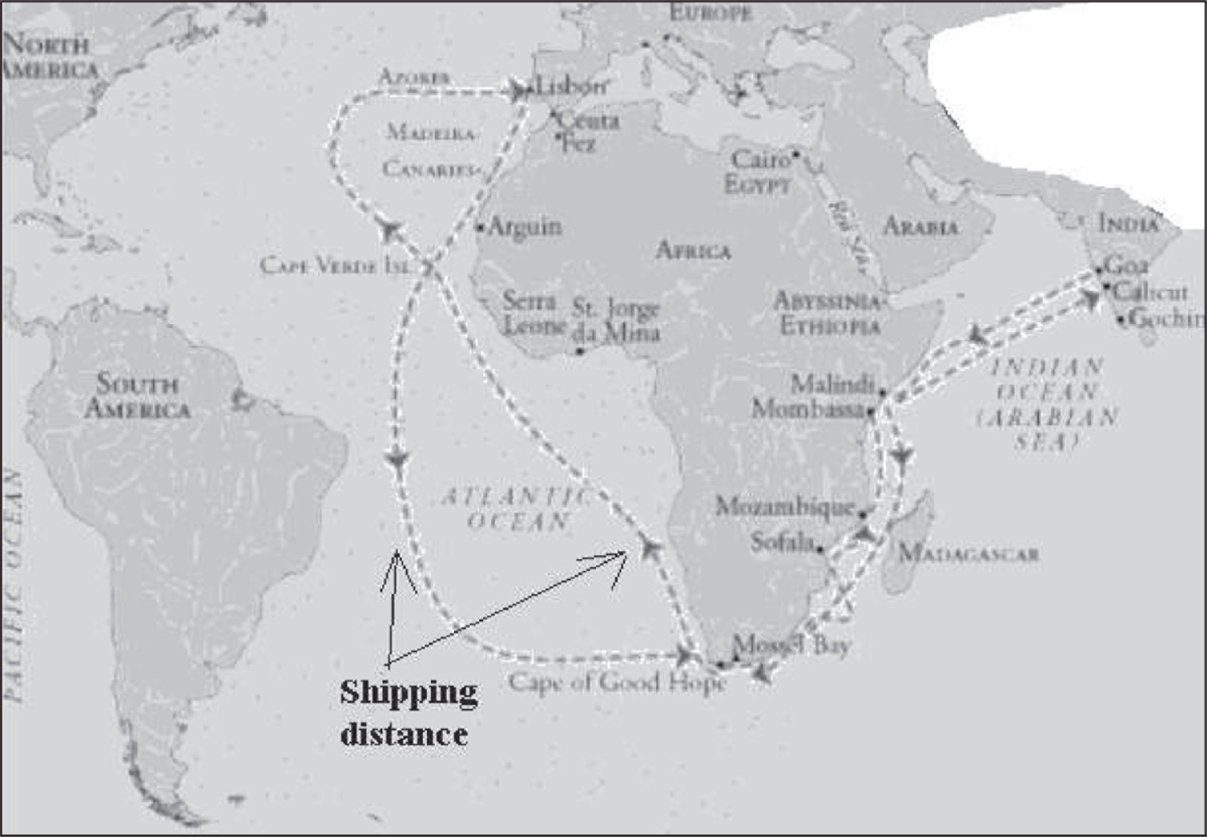
Illustration 6. Air distance between two countries X and Y is shown in Figure 5.

Shipping distance between two countries: It is the distance, $D_{i, j}^{s h i p}$ , between two points (basically, ports) P_i and P_j measured along a straight line or curved path or their mixed paths that is, along the path of movement of the ship,

where,

P_i = a port (e.g., source/destination) of the country i,

P_j = a port (e.g., destination/source) of the country j.

Illustration 7. Shipping distance between two countries X and Y is shown in Figure 6.

Figure 4.

Source: www.printablee.com

Figure 5.

Source: www.printablee.com

Figure 6.

Source: iasshiksha.blog

Road distance between two countries: It is the distance, $D_{i, j}^{r o a d}$ , between two connected points P_i and P_j by road and is measured along the road ways, that is, along the way the cargo moves,

where,

P_i = location of a transport (e.g., source/destination) of the country i,

P_j = location of a transport (e.g., destination/source) of the country j.

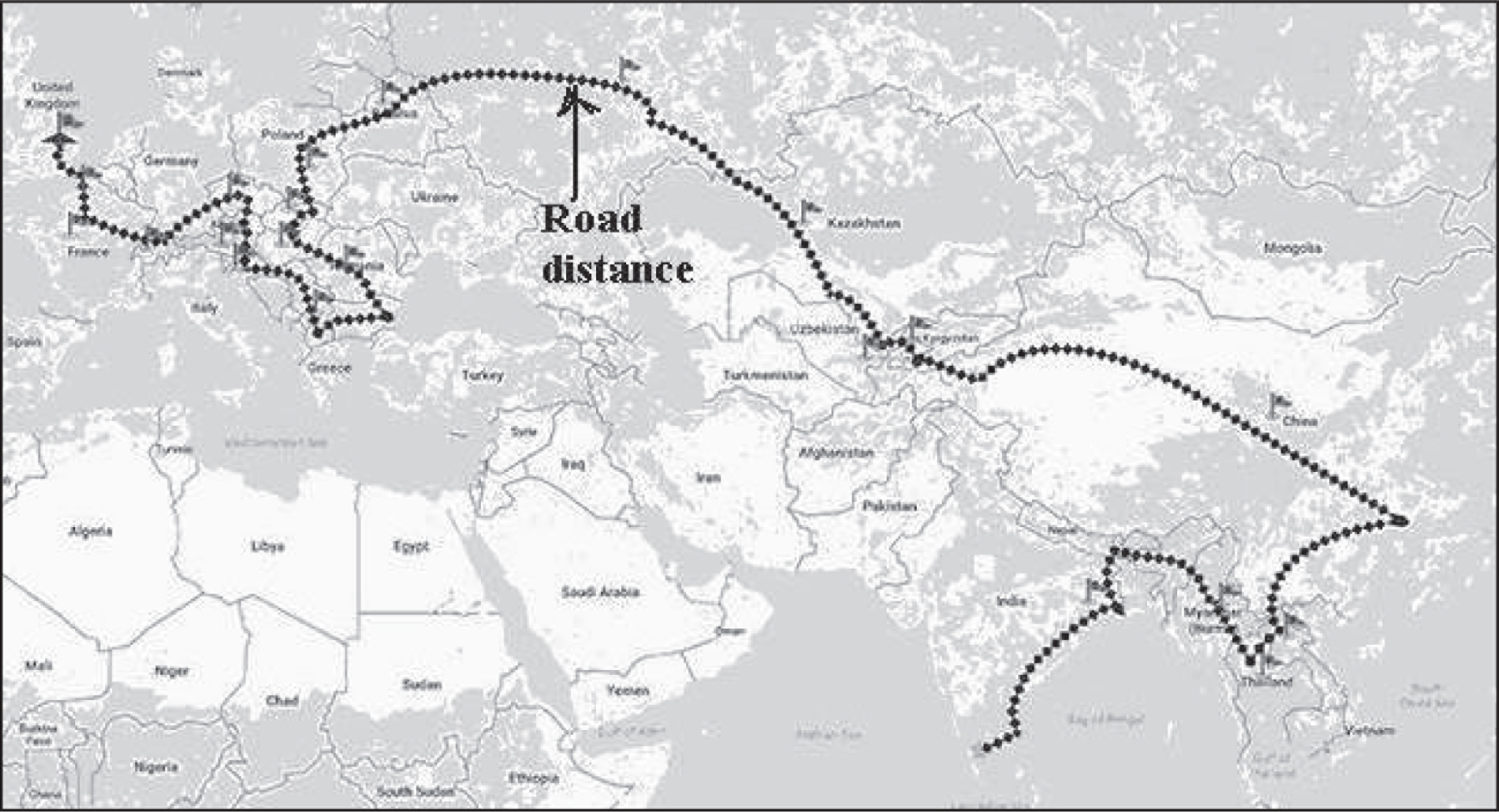
Illustration 8. Road distance between two countries X and Y is shown in Figure 7.

Geographical distance between two countries: In general it is any of the above distances measured along the path on the globe between two countries and is denoted by D_i,j, as distance between country i and country j. In standard gravity model analyses, the distance between the capital cities of both the countries are commonly used.

Role of Shipping Cost in Gravity Models

Primarily the shipping cost of goods between country i and country j directly depends on the distance D_i,j between them. Therefore the force of trade flow between country i and country j decreases as the shipping cost increases when the mode of shipping is same. Again, the shipping cost of goods depends on mode of transport and the size of the ship (e.g., small, medium, large) (Hummels, 1999) as well as the volume of goods to be transported.

Figure 7.

Source: www.thenewsminute.com

Illustration 9. Consider three countries such as country i, country j and country k where the distance D_i,j > D_i,k, and the economic mass M_j = M_k then by gravity model, the force of trade flow F_i,j < F_i,k. If we change the mode of shipping for the same volume of goods from country i to country j and from country i to country k in such a way that their shipping cost is same. Then, the gravity model also computes that the force of trade flow F_i,j < F_i,k. But in the true sense we feel that the expected force of trade flow $F_{i, j} ≅ F_{i, k}$ , provided the size of the ship.

\begin{matrix} Discussion: We know F_{i j} = \frac{M_{i} M_{j}}{D_{i j}^{2}} a n d F_{i k} = \frac{M_{i} M_{k}}{D_{i k}^{2}} \\ Therefore, \frac{F_{i j}}{F_{i k}} = \frac{M_{i} M_{j}}{D_{i j}^{2}} \frac{D_{i k}^{2}}{M_{i} M_{k}} \\ or, \frac{F_{i j}}{F_{i k}} = \frac{D_{i k}^{2}}{D_{i j}^{2}} \frac{M_{i} M_{j}}{M_{i} M_{k}} \end{matrix}

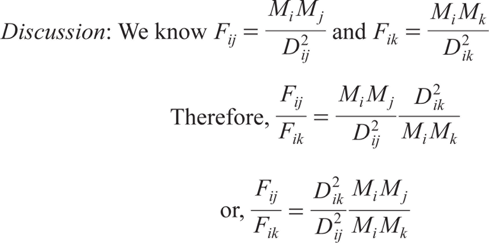
when M_j = M_k

\frac{F_{i j}}{F_{i k}} = \frac{D_{i k}^{2}}{D_{i j}^{2}} .

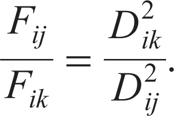
If D_ij > D_ik, that is, $\frac{D_{i k}}{D_{i j}} \leq 1$ , then $\frac{F_{i j}}{F_{i k}} \leq 1$ , that is, F_ij < F_ik.

Here M_j = M_k but the loading and unloading cost of goods in a ship is a major part of the cost other than cost of sea transport. If the distance is more and also the size of the ship is large, then there is not much effect on trade force of attraction. In this context, we can say that F_ij ≈ F_ikwhen M_j = M_k.

By Illustration 9, it is justified that shipping cost is more appropriate than physical distance in the gravity model of international trade. Now, if we replace D_i,j in the gravity model described in Equation (10) by the shipping cost T_i,j then, the modified gravity model can be described as in Equation (11).

\ln X_{i, j, t} = b_{0} + b_{1} \ln Y_{i, t} + b_{2} \ln Y_{j, t} + b_{3} \ln T_{i, j} + e_{i, j},

(11)

where,

Y_i,t = Economic mass for country i at time t,

Y_j,t = Economic mass for country j at time t,

T_i,j = Shipping cost from country i to country j,

X_i,j,t = Force of trade flow between country i and country j at time t,

e_i,j = Random error term when trade flow between country i and country j

E(e_i,j) = expected value of e_i,j

= 0

b₀, b₁, = Parameters of the model in

b₂, b₃ which b₃ < 0 since ‘distance is negatively proportional to the trade force’.

Effect of Common Border in Gravity Model

In case of two adjacent countries, with a common border, the shortest distance between them is zero but the geographical distance is not zero in the gravity model because the geographical distance is the length of path on which goods flow between the adjacent countries. Depending on whether the common border is land, or water body, the trade cost would be calculated according to the above specifications. The gravity model described in Equation (11) would suitably use the shipping cost as equivalent to distance.

Generally, in order to consider border as a factor in the gravity model, we introduce two dummy variables.

One for common border

Other border types

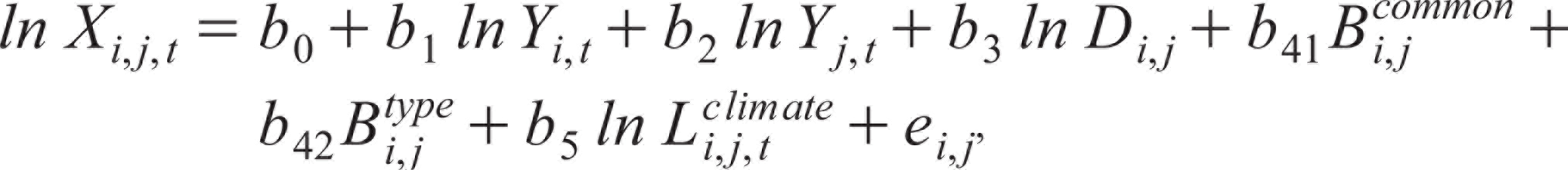
Then the gravity model in Equation (11) is modified and described in Equation (12).

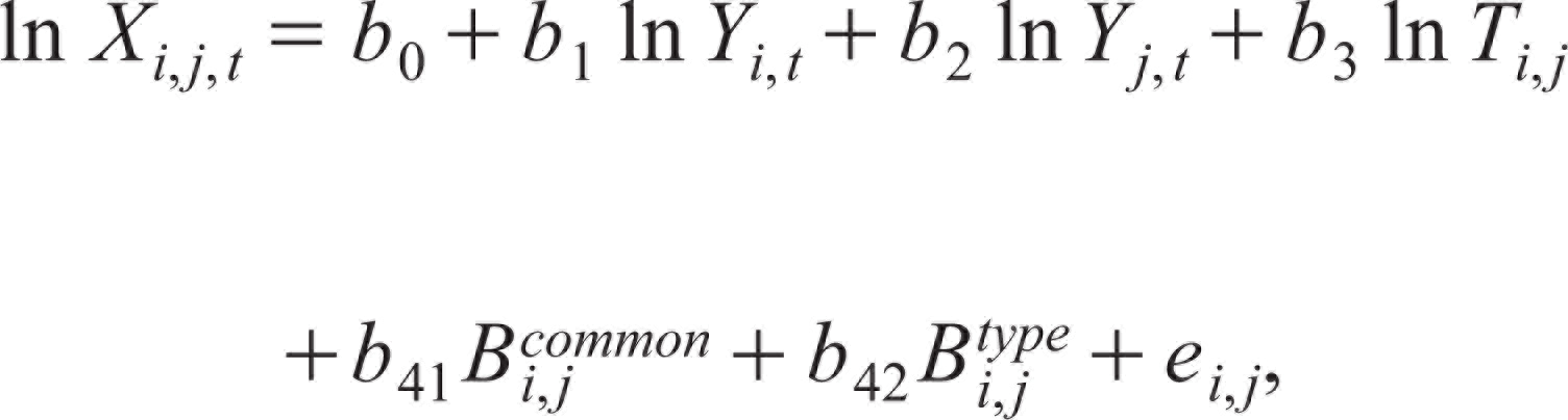
\begin{matrix} \ln X_{i, j, t} = b_{0} + b_{1} \ln Y_{i, t} + b_{2} \ln Y_{j, t} + b_{3} \ln T_{i, j} \\ + b_{41} B_{i, j}^{c o m m o n} + b_{42} B_{i, j}^{t y p e} + e_{i, j}, \end{matrix}

(12)

where,

$B_{i, j}^{c o m m o n} = {\begin{matrix} 1, & c o u n t r y_{i} a n d c o u n t r y_{j} w i t h c o m m o n b o r d e r \\ 0, & c o u n t r y_{i} a n d c o u n t r y_{j} w i t h n o c o m m o n b o r d e r \end{matrix}$

$B_{i, j}^{t y p e} = {\begin{matrix} 1, & c o u n t r y_{i} a n d c o u n t r y_{j} w i t h s e a b o r d e r \\ 0, & c o u n t r y_{i} a n d c o u n t r y_{j} w i t h n o s e a b o r d e r \end{matrix}$

b₄₁, b₄₂ = parameters related to border in the model

Role of Climate in Gravity Model

As the distance between the partner countries increases, the travelling time to transport of goods also increases. In other words, vessel carrying goods float longer time on the deep sea, often exposing these to adverse climatic conditions and increasing the probability of losses (introduced as a loss parameter) due to damages, delays and additional costs due to hold ups, etc. Despite access to well laid out insurance contracts for the freight, historically speaking, the distance poses a natural barrier to trade between far-off countries, especially via sea routes, automatically lowering the force of business attraction.

So, one can incorporate the climate variable in the gravity model. Subsequently, Equation (12) can be rewritten as Equation (13).

\begin{matrix} \ln X_{i, j, t} = b_{0} + b_{1} \ln Y_{i, t} + b_{2} \ln Y_{j, t} + b_{3} \ln D_{i, j} + b_{41} B_{i, j}^{c o m m o n} + \\ b_{42} B_{i, j}^{t y p e} + b_{5} \ln L_{i, j, t}^{c \lim a t e} + e_{i, j,} \end{matrix}

(13)

where,

D_ij = Distance between country i to country j along the path of shipping by the ship

$L_{i, j, t}^{c \lim a t e}$ = Economic loss during shipping of goods from country i to country j at time t

b₅ = a parameter of the model.

Role of Demography in Gravity Model

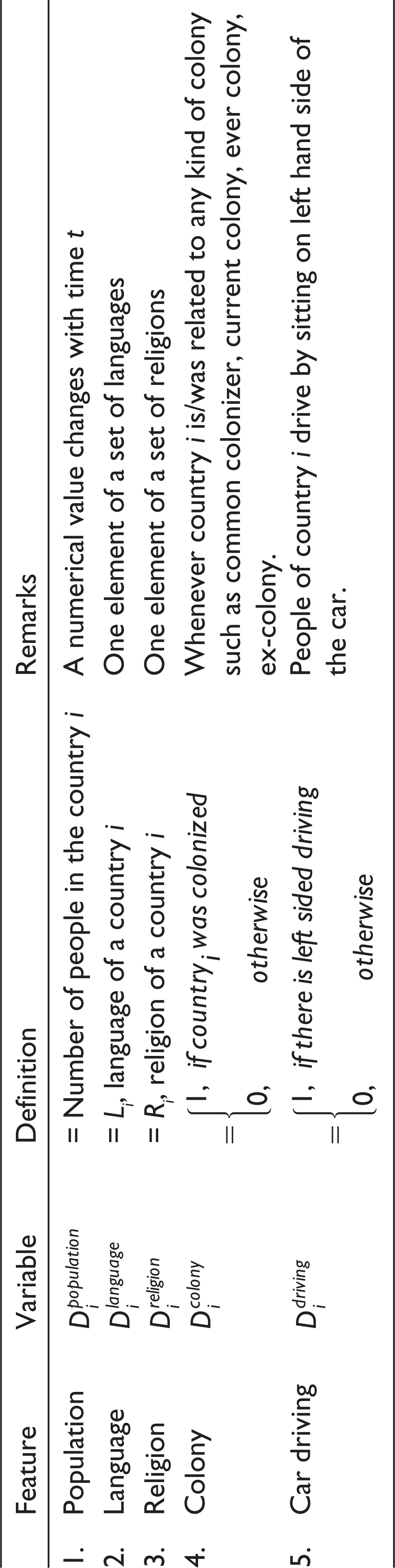
Demographic information of a country means population, language, religion, food habit, etc. Country-specific demographic features of a country are as follows:

Population

Language

Religion

Culture

Nation

Colonizer

Internal political tension

War

Car driving pattern, etc.

Now we briefly describe below some of these features or variables for a country, say country i and summarize it in Table 1.

While, the population size and language for communication are important considerations, for example trade with a sparsely populated country, or very difficult to communicate type of country would be low, common religion and culture have a mixed influence on the countries in international trade networks. It has been observed that the sharing of Buddhist, Confucian, Hindu, Eastern Orthodox Catholic, etc., religion in different countries have a significantly positive influence on bilateral trade. Moreover, religious openness has a strong positive effect on trade. Trade, in general, is influenced differently by every religious belief (Helble, 2006). For example Islam has stronger influence on trade than Christianity due to their indigenous religious beliefs. Similarly, Hindus trading among each other have a statistically insignificant relationship. Jews prefer trading among themselves, whereas Buddhists avoid trade with people of same religion (Helble, 2006). On a different note, war and war-like situations (see, Anderton & Carter, 2001; Bayer & Rupert, 2004; Misra & Choudhry, 2020) lead to loss of international trade.

Subsequently, the gravity model in Equation (13) can be modified by incorpating population, language and religion as shown in Equation (14).

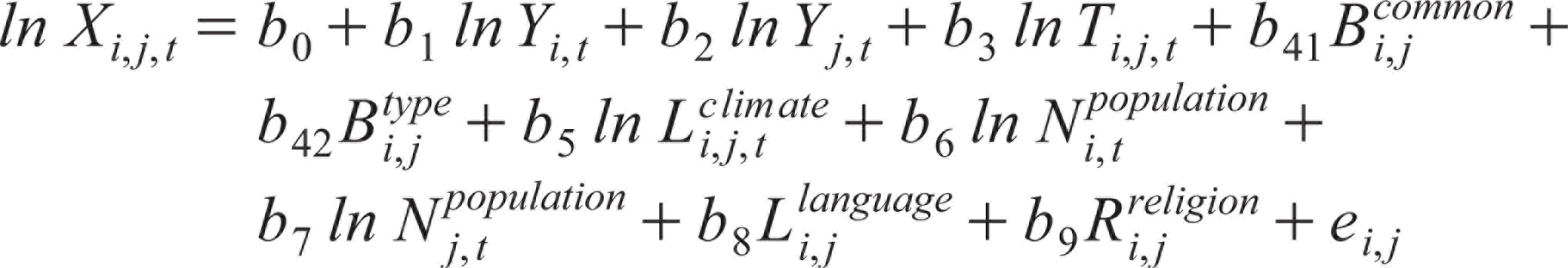
\begin{matrix} \ln X_{i, j, t} = b_{0} + b_{1} \ln Y_{i, t} + b_{2} \ln Y_{j, t} + b_{3} \ln T_{i, j, t} + b_{41} B_{i, j}^{c o m m o n} + \\ b_{42} B_{i, j}^{t y p e} + b_{5} \ln L_{i, j, t}^{c \lim a t e} + b_{6} \ln N_{i, t}^{p o p u l a t i o n} + \\ b_{7} \ln N_{j, t}^{p o p u l a t i o n} + b_{8} L_{i, j}^{l a n g u a g e} + b_{9} R_{i, j}^{r e l i g i o n} + e_{i, j} \end{matrix}

(14)

where,

$N_{i, t}^{p o p u l a t i o n}$ = Population of country i at time t,

L_i = Language of a country i

$L_{i, j}^{l a n g u a g e}$ = ${\begin{matrix} 1, & L_{i} = L_{j} \\ 0, & L_{i} \neq L_{j} \end{matrix}$

R_i = Religion of country i

$R_{i, j}^{r e l i g i o n} = {\begin{matrix} 1, R_{i} = R_{j}, \\ R_{i} = R_{j} ε S_{1} \\ 0, R_{i} = R_{j}, \\ R_{i} = R_{j} ε S_{2} \\ - 1, R_{i} = R_{j}, \\ R_{i} = R_{j} ε S_{3} \end{matrix}$

b₉ = Parameter of the model related to religion and culture,

Table 1.

Country-specific Demographical Features for the Country i

	Feature	Variable	Definition	Remarks
1.	Population	$D_{i}^{p o p u l a t i o n}$	= Number of people in the country i	A numerical value changes with time t
2.	Language	$D_{i}^{l a n g u a g e}$	= L_i, language of a country i	One element of a set of languages
3.	Religion	$D_{i}^{r e l i g i o n}$	= R_i, religion of a country i	One element of a set of religions
4.	Colony	$D_{i}^{c o l o n y}$	$= {\begin{matrix} 1, & i f c o u n t r y_{i} w a s c o l o n i z e d \\ 0, & o t h e r w i s e \end{matrix}$	Whenever country i is/was related to any kind of colony such as common colonizer, current colony, ever colony, ex-colony.
5.	Car driving	$D_{i}^{d r i v i n g}$	$= {\begin{matrix} 1, & i f t h e r e i s l e f t s i d e d d r i v i n g \\ 0, & o t h e r w i s e \end{matrix}$	People of country i drive by sitting on left hand side of the car.

Source: The authors.

where, for example,

S₁ = {Buddhist, Confucian, Hinduism, Eastern Orthodox Catholic}

S₂ = {Islam, Judaism}

S₃ = {Roman Catholic}.

Measures of Remoteness (or Nearness) in Gravity Models

Some features are computed based on the present trading (international) position of a country. A country i is trading with her partner countries at time t. That means country i is trading with a set of countries at time t but at time t + 1 the set of country may not be the same. Country-specific dynamic dependent features are the features of a country which depends on other countries and it also changes from time to time. Some features of this kind are listed below.

Remoteness (Nearness)

Similarity

Similarity in country size

Similarity between countries

Similarity in income

Similarity in economic sizes

Relative factors

Average tariffs

Differences in per capita income

Trade orientation, trade imbalance, economies of scale

Level of infrastructure

Multilateral trade resistance

Information costs

Remoteness

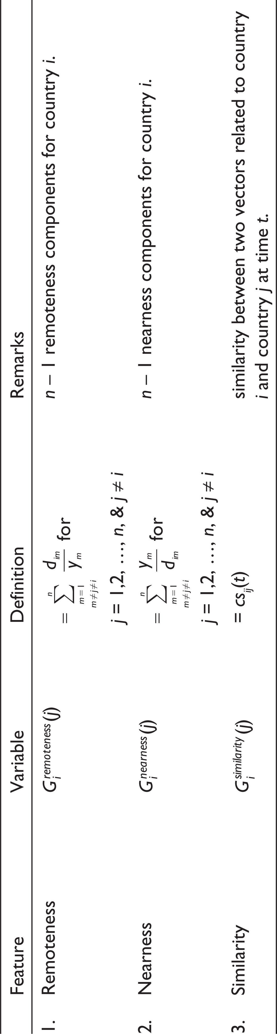
Remoteness as a factor is introduced by Anderson and Wincoop (2003) and is related to the study of gravity model of international trade. Remoteness is defined as follows.

It is a competitive feature/factor between two partner countries with respect to other partner countries in international trade. This is an indicator of willingness of trade flow between two countries in their trading network. The remoteness of country i with respect to country j is defined as follows:

R E M_{i} = \sum_{m \neq j} \frac{d_{i m}}{y_{m}},

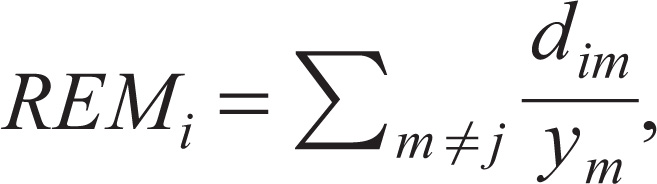
where

y_m = GDP of country m, for m = 1,2,…,n

D_im = Distance of country m from country i for m = 1,2,…,n, & m  i

So the remoteness variable is intended to reflect the average distance of country i from all trading partners other than country j.

Computation of Remoteness

Suppose there are n countries in a trade network. We want to compute remoteness for country i with respect to country j for j = 1,2, …,n and j  i. In this situation country i has n – 1 partner countries for trading. So country i has n – 1 remoteness values for its partner countries. Therefore remoteness of country i is a vector of size n – 1. Computational formula of remoteness of country i is given in Equation (15).

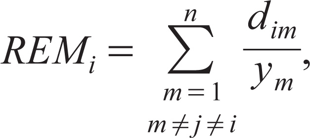
R E M_{i} = \sum_{\begin{matrix} m = 1 \\ m \neq j \neq i \end{matrix}}^{n} \frac{d_{i m}}{y_{m}},

(15)

for j = 1,2, …, n, & j  i

where

y_m = GDP of country_m, for m = 1,2, …, n

D_im = Distance of country_m from country i for m = 1,2, …, n, & m  i

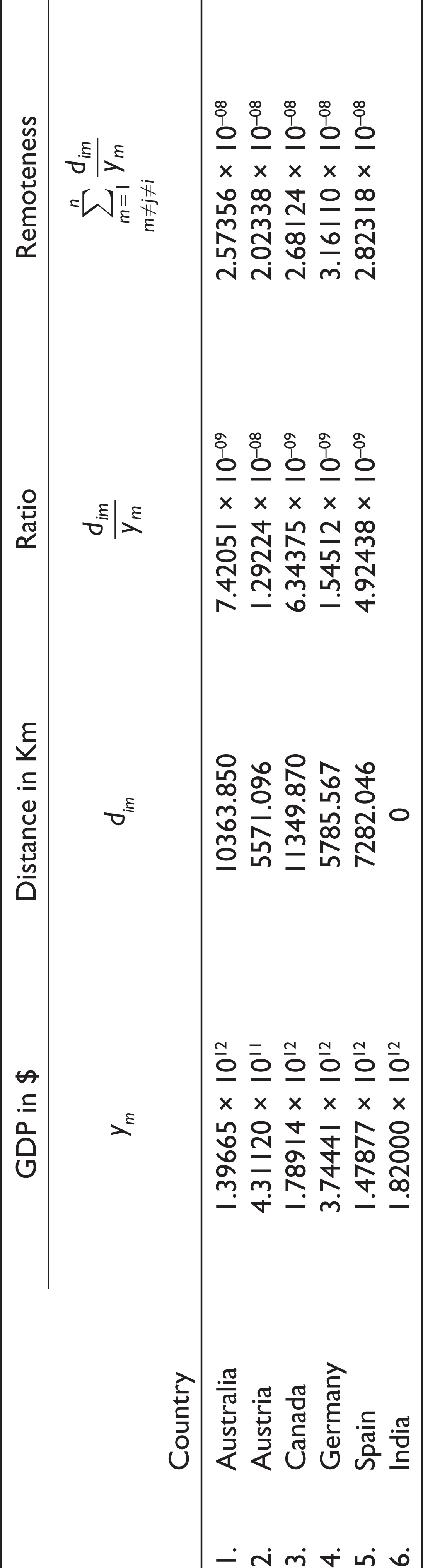
A numerical example for the computation of remoteness for a country is given in Illustration 10.

Illustration 10. In 2011, the partner countries of India were Australia, Austria, Canada, Germany, and Spain. The GDP of each country in international trade for the year 2011 and their distance from India are given in Table 2. Now the computation of remoteness variable of India for a country such as Australia, Austria, Canada, Germany or Spain is given in Table 2.

Now the remoteness of India for Australia is ^–08^–09^–09^–09^–08

Similarly the remoteness of India for Austria is ^–09^–09^–09^–09^–08

Remoteness of India for Canada is ^–08^–09^–09^–09^–08

Ñ The remoteness of India is a vector as ^–08^–08^–08^–08^–08

Illustration 11. In 2011, the partner countries of Spain were Australia, Austria, Canada, Germany, and India. The GDP of each country in the international trade for the year 2011 and their distance from Spain are given in Table 3. The computation of remoteness variable of Spain for a country such as Austria, Canada, Germany or India is given in Table 3.

Table 2.

GDP and Distance from India for 2011

	Country	GDP in $	Distance in Km	Ratio	Remoteness
	Country	y_m	d_im	$\frac{d_{i m}}{y_{m}}$	$\begin{matrix} \sum_{m =1}^{n} \frac{d_{i m}}{y_{m}} \\ m \neq j \neq i \end{matrix}$
1.	Australia	1.39665 × 10¹²	10363.850	7.42051 × 10^–09	2.57356 × 10^–08
2.	Austria	4.31120 × 10¹¹	5571.096	1.29224 × 10^–08	2.02338 × 10^–08
3.	Canada	1.78914 × 10¹²	11349.870	6.34375 × 10^–09	2.68124 × 10^–08
4.	Germany	3.74441 × 10¹²	5785.567	1.54512 × 10^–09	3.16110 × 10^–08
5.	Spain	1.47877 × 10¹²	7282.046	4.92438 × 10^–09	2.82318 × 10^–08
6.	India	1.82000 × 10¹²	0

Source: The authors.

Table 3.

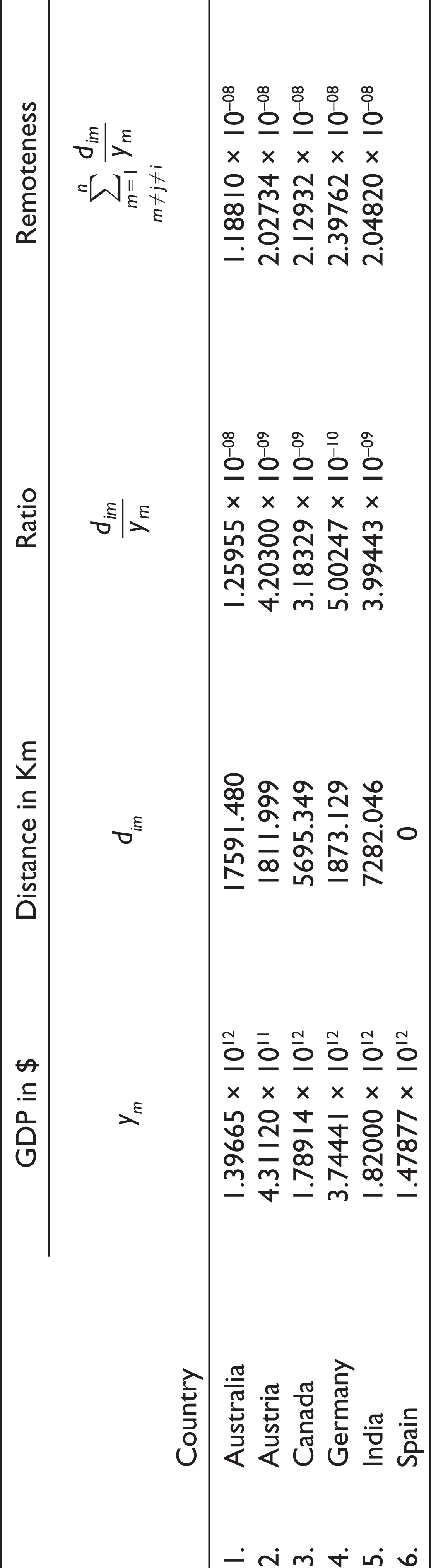
GDP and Distance from Spain for 2011

	Country	GDP in $	Distance in Km	Ratio	Remoteness
	Country	y_m	d_im	$\frac{d_{i m}}{y_{m}}$	$\begin{matrix} \sum_{m =1}^{n} \frac{d_{i m}}{y_{m}} \\ m \neq j \neq i \end{matrix}$
1.	Australia	1.39665 × 10¹²	17591.480	1.25955 × 10^–08	1.18810 × 10^–08
2.	Austria	4.31120 × 10¹¹	1811.999	4.20300 × 10^–09	2.02734 × 10^–08
3.	Canada	1.78914 × 10¹²	5695.349	3.18329 × 10^–09	2.12932 × 10^–08
4.	Germany	3.74441 × 10¹²	1873.129	5.00247 × 10^–10	2.39762 × 10^–08
5.	India	1.82000 × 10¹²	7282.046	3.99443 × 10^–09	2.04820 × 10^–08
6.	Spain	1.47877 × 10¹²	0
Ñ The remoteness of Spain is a vector as
(1.18810 × 10^–08, 2.02734 × 10^–08, 2.12932 × 10^–08, 2.39762 × 10^–08, 2.04820 × 10^–08)

Source: The authors.

Note: The remoteness of India for Spain is 2.82318 × 10^–08 (Illustration 10) and remoteness of Spain for India is 2.04820 × 10^–08 (Illustration 11).

Anderson and Wincoop (2003) stated that commonly used remoteness variables are entirely disconnected from the theory. They showed that adding remoteness indices for both country i and country j changes the border coefficient estimates very little and also has very little additional explanatory power.

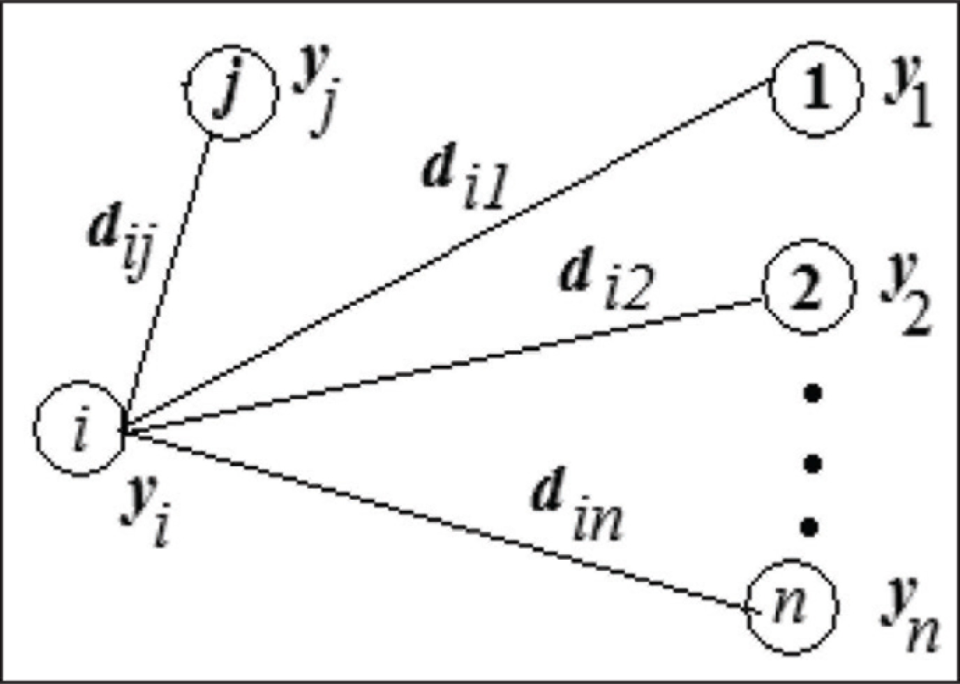
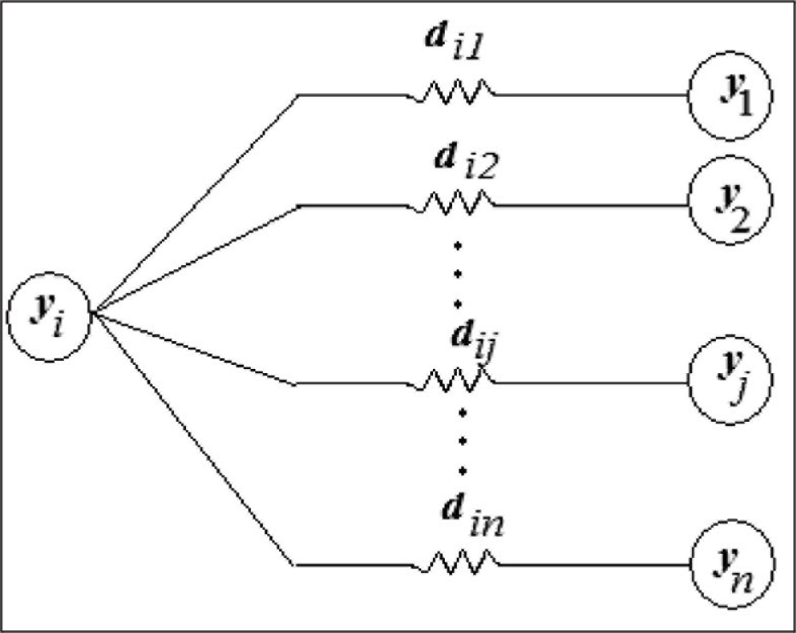
Given that country i is a member of a trading network with n countries, country i has n – 1 partner countries. The relation of country i with other n – 1 partner countries is shown in Figure 8.

In Figure 8,

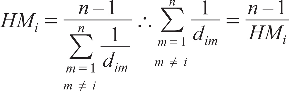
y_m = GDP of country m, for m = 1,2,…, n

d_im = Distance of country m from country i for m = 1,2,…, n, & m  i

HM_i = Harmonic mean of distances for country i

By the definition of harmonic mean (HM) for the quantities (x₁,x₂,…, x_n) we can write

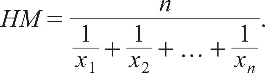
H M = \frac{n}{\frac{1}{x_{1}} + \frac{1}{x_{2}} + \dots + \frac{1}{x_{n}}} .

Now we apply the definition of harmonic mean (HM) for the distances d_im for m = 1,2,…, n, m  i then

\begin{matrix} H M_{i} = \frac{n - 1}{\sum_{m = 1}^{n} \frac{1}{d_{i m}}} ∴ \sum_{m = 1}^{n} \frac{1}{d_{i m}} = \frac{n - 1}{H M_{i}} \\ m \neq i ​ ​ ​ ​ ​ ​ ​ ​ ​ ​ ​ ​ ​ ​ ​ ​ ​ ​ ​ ​ ​ ​ ​ ​ ​ ​ ​ ​ ​ ​ m \neq i \end{matrix}

(16)

Figure 8.

Source: The authors.

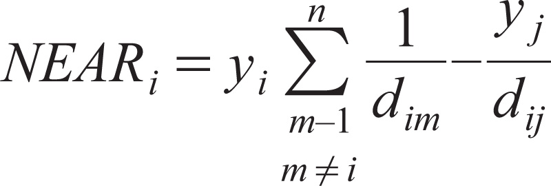
As opposed to the Remoteness of a country, the following definition serves as a measure of the Nearness for country i with respect to country 1 as:

N E A R_{i} (1) = \sum_{m = 2}^{n} \frac{y_{m}}{d_{i m}} .

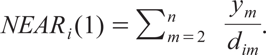
Similarly, value of nearness for country i with respect to country j is

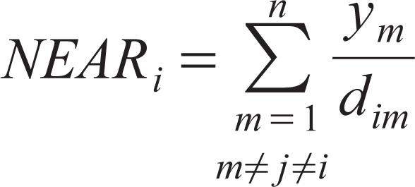
\begin{matrix} N E A R_{i} = \sum_{m = 1}^{n} \frac{y_{m}}{d_{i m}} \\ m ​ \neq ​ j ​ \neq ​ i \end{matrix}

(17)

for j = 1,2, …,n & j  i.

However, this neraness network has a strong analogy with the electrical network. The following sub-section elaborates on this relation.

An Analogy with Electrical Network

Each country of a trade network may be considered as a node of an electrical network. The GDP of a country is equivalent to a voltage of that node, that is, voltage potential of the node. Similarly, the distance between two countries is equivalent to resistance between the corresponding nodes. The equivalent electrical circuit corresponding to the part of trade network (Figure 8) is shown in Figure 9.

Figure 9.

Source: The authors.

Now we analyse the ith node whose potential is y_i. Here, we consider the following.

Current is always flowing from higher potential to lower potential.

If current is negative then it flows in the reverse direction.

Ohm’s Law:

c u r r e n t = \frac{p o t e n t i a l d i f f e r e n c e}{r e s i s ​ \tan ​ c e}

Consider the node i and node 1 where resistance between the nodes is d_i₁ and assume that y₁ is higher voltage than y_i. Therefore, the potential difference = y₁ – y_i

Now by Ohms law we get

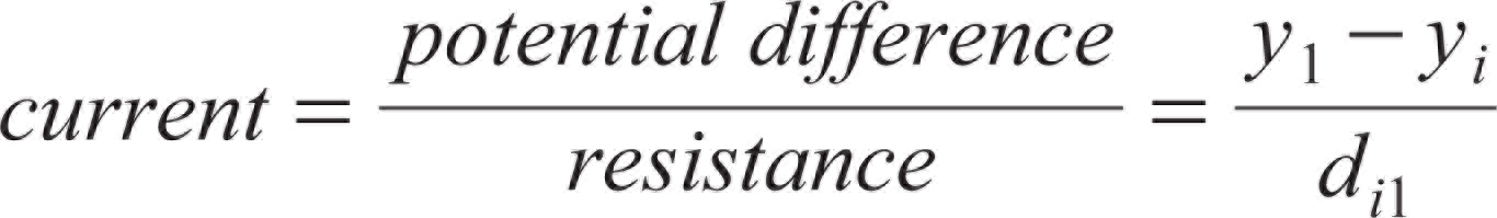
c u r r e n t = \frac{p o t e n t i a l d i f f e r e n c e}{r e s i s ​ \tan ​ c e} = \frac{y_{1} - y_{i}}{d_{i 1}}

is flowing from node 1 to node i .

In addition, Kirchhoff’s current law says that

In an electrical network, the algebraic sum of currents meeting at a point (i.e., node) is zero.

Therefore, we can write as

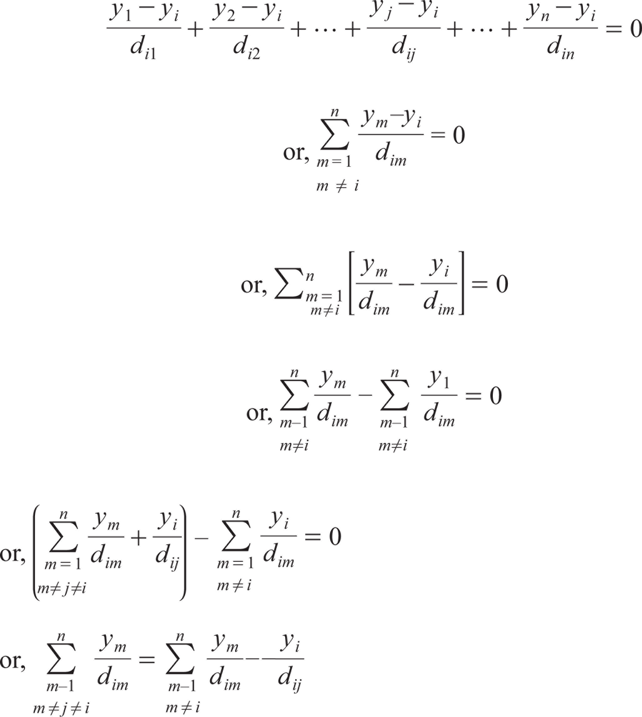
\begin{matrix} \frac{y_{1} - y_{i}}{d_{i 1}} + \frac{y_{2} - y_{i}}{d_{i 2}} + \dots + \frac{y_{j} - y_{i}}{d_{i j}} + \dots + \frac{y_{n} - y_{i}}{d_{i n}} = 0 \\ o r, \begin{matrix} {\sum^{​}}_{n}^{m = 1} \frac{y_{m} - y_{i}}{d_{i m}} = 0 \\ m \neq i \end{matrix} \\ o r, {\sum^{​}}_{n}^{\underset{m \neq i}{m = 1}} [\frac{y_{m}}{d_{i m}} - \frac{y_{i}}{d_{i m}}] = 0 \\ o r, \begin{matrix} {\sum^{​}}_{n}^{m - 1} \frac{y_{m}}{d_{i m}} ​ ​ ​ - {\sum^{​}}_{n}^{m - 1} \frac{y_{1}}{d_{i m}} = 0 \\ m ​ \neq ​ i ​ ​ ​ ​ ​ ​ ​ ​ ​ ​ ​ ​ ​ ​ ​ ​ ​ ​ ​ ​ ​ ​ ​ ​ ​ ​ ​ ​ m ​ \neq ​ i ​ \end{matrix} \\ o r, (\begin{matrix} {\sum^{​}}_{n}^{m = 1} \frac{y_{m}}{d_{i m}} + \frac{y_{i}}{d_{i j}} \\ m ​ \neq ​ j ​ \neq ​ i \end{matrix}) - {\sum^{​}}_{n}^{\begin{matrix} m = 1 \\ m \neq i \end{matrix}} \frac{y_{i}}{d_{i m}} = 0 \\ o r, {\sum^{​}}_{n}^{\begin{matrix} m - 1 \\ m \neq j \neq i \end{matrix}} \frac{y_{m}}{d_{i m}} = {\sum^{​}}_{n}^{\begin{matrix} m - 1 \\ m \neq i \end{matrix}} \frac{y_{m}}{d_{i m}} - - \frac{y_{i}}{d_{i j}} \end{matrix}

Now by using Equation (16), we get

\begin{matrix} N E A R_{i} = y_{i} {\sum^{​}}_{n}^{\begin{matrix} m - 1 \\ m \neq i \end{matrix}} \frac{1}{d_{i m}} - \frac{y_{j}}{d_{i j}} \\ o r, N E A R_{i} = y_{​} \frac{n - 1}{H M_{i}} - \frac{y_{j}}{d_{i j}} [u \sin g E q u a t i o n (17)] \end{matrix}

\begin{matrix} ∴ N E A R_{i} = \frac{(n - 1) y_{i}}{H M,} - \frac{y_{j}}{d_{i j}} \\ ∴ N E A R_{i} = \frac{(n - 1) y_{i}}{H M_{i}} - \frac{y_{j}}{d_{i j}} \end{matrix}

(18)

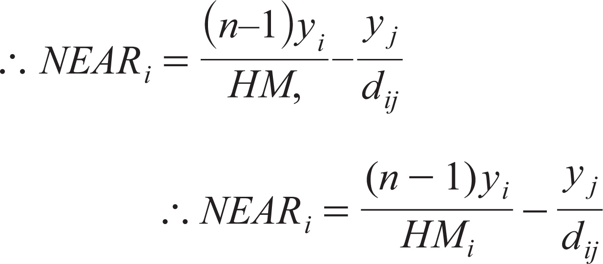
Now using Equations (17) and (18) we get

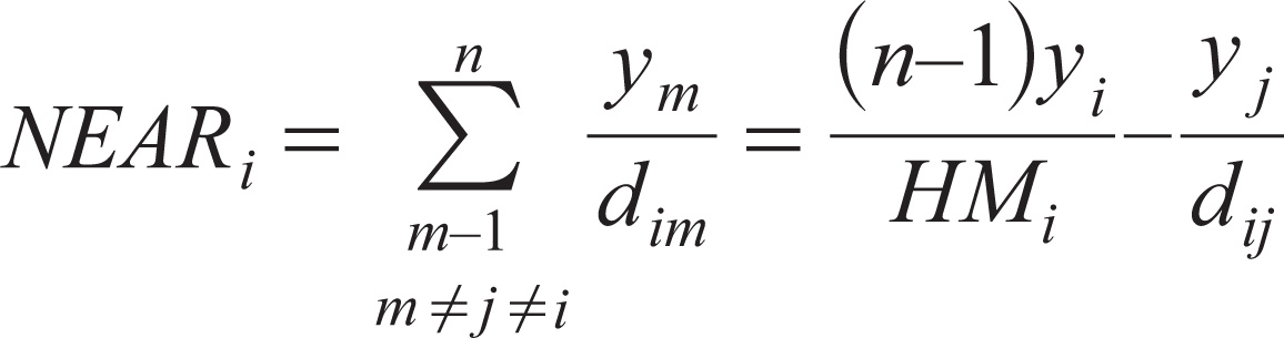
N E A R_{i} = \sum_{\begin{matrix} m - 1 \\ m \neq j \neq i \end{matrix}}^{n} \frac{y_{m}}{d_{i m}} = \frac{(n - 1 ​) y_{i}}{H M_{i}} - \frac{y_{j}}{d_{i j}}

for j = 1,2, …,n, & j  i

Finally, in international economics, the similarity factor in country size or country size related similarity are used by different researchers such as Egger (2002, 2004), Pridy (2005), Antonucci and Manzocchi (2006), and others. The measure of similarity between countries is an explanatory variable in the models and a country can be represented by a l -dimensional vector, where each component of this vector belongs to any of the following domains (a) geographical parameters, (b) demographical parameters, (c) economic parameters, etc., even some computed parameters in a time frame.

Table 4.

Country-specific Dynamic Dependent Features for Country i at Time t

	Feature	Variable	Definition	Remarks
1.	Remoteness	$G_{i}^{r e m o t e n e s s} (j)$	$= \sum_{\begin{matrix} m =1 \\ m \neq j \neq i \end{matrix}}^{n} \frac{d_{i m}}{y_{m}} for$ j = 1,2, …, n, & j ¹ i	n – 1 remoteness components for country i.
2.	Nearness	$G_{i}^{n e a r n e s s} (j)$	$= \sum_{\begin{matrix} m =1 \\ m \neq j \neq i \end{matrix}}^{n} \frac{y_{m}}{d_{i m}} for$ j = 1,2, …, n, & j ¹ i	n – 1 nearness components for country i.
3.	Similarity	$G_{i}^{s i m i l a r i t y} (j)$	= cs_ij(t)	similarity between two vectors related to country i and country j at time t.

Source: The authors.

Summary of Country-specific Dynamic Dependent Features

In this section, we have summarized various country-specific dynamic dependent features/factors as shown in Table 4.

Conclusion

The present article is a selective review of the relation between the laws of physics and those adopted by the theory and applications of gravity models in international trade. We tried to exemplify through various possible angles, the overarching relations between Newton’s Law and the structure constructed for understanding the scope and dimensions of bilateral trade between countries that differ according to a host of criteria.

To begin with, we drew parallels between the core components of the two theories and subsequently panned out the constituent elements that keep the gravity equations in international trade in close resemblance to the celebrated natural laws. Indeed, the classical and time-tested theories in international trade do not usually engage with factors that offer salient characteristics to the gravity model. Components such as the size of countries engaging in trade, the distance between the countries—which we subsequently comprehend into a discussion on remoteness and nearness—and the cultural, religious and even colonial relations developed over centuries provide crucial ingredients to re-estimate the observed patterns of trade at bilateral and multilateral levels.

We used the indices of remoteness and nearness to reflect on trade between India and some of the European countries and generally tried to offer a unified treatment of the early gravity models and the more recent versions, where, as we have also pointed out clearly, the empirical realities find explanations in product differentiated models of trade, in love for variety and in differences between factor proportions across countries. Overall, it is perhaps not surprising that Newton’s Law or Ohm’s Law have a lot of commonality with the theoretical predictions in trade models, but to the extent these principles find empirical validity and generate a much bigger appeal beyond the limited applications, is useful for the conceptual sphere of the subject in an increasingly multidisciplinary research environment.

Footnotes

Acknowledgements

The authors thank an anonymous reviewer for very useful suggestions. The remaining errors are our own.

Declaration of Conflicting Interests

The authors declared no potential conflicts of interest with respect to the research, authorship and/or publication of this article.

Funding

The authors received no financial support for the research, authorship and/or publication of this article.

References

Anderson

J. E.

(1979). A theoretical foundation of the gravity model. American Economic Review, 69(1), 106–116.

Anderson

J. E.

, & Wincoop

E. V.

(2003). Gravity with gravitas: A solution to the border puzzle. American Economic Review, 93(1), 170–192. https://doi.org/10.1257/000282803321455214.hdl:10532/3989

Anderson

J. E.

, & Wincoop

E. V.

(2004). Trade costs. Journal of Economic Literature, 42(3), 691–751.

Anderton

C. H.

, & Carter

J. R.

(2001). The impact of war on trade: An interrupted time-series study. Journal of Peace Research. http://doi.org/10.1177/0022343301038004003

Antonucci

, & Manzocchi

(2006). Does Turkey have a special trade relation with the EU? A gravity model approach. Economic Systems, 30(2), 157–169.

Baldwin

, & Taglioni

(2006). Gravity for dummies and dummies for gravity equations. (NBER Working Paper No. 12516). NBER.

Bergstrand

J. H.

(1985). The gravity equation in international trade: Some microeconomic foundations and empirical evidence. The Review of Economics and Statistics, 67(3), 474–481. https://doi.org/10.2307/1925976.JSTOR1925976

Bergstrand

(1989). The generalized gravity equation, monopolistic competition, and the factor-proportions theory in international trade. The Review of Economics and Statistics, 71, 143–153.

Chaney

(2008). Distorted gravity: The intensive and extensive margins of international trade. American Economic Review, 98(4), 1707–1721.

10.

Davies

(1995). Local economies and globalization (Note Book N 20). OECD.

11.

Deardorff

A. V.

(1998). Determinants of bilateral trade: Does gravity work in a neoclassical world? In Frankel

J. A.

(Eds.), The regionalization of the world economy (p. 21). University of Chicago Press.

12.

Dhar

, & Panagariya

(1994). Predictions of bilateral trade and the gravity equation (Working Paper). International Trade Division, World Bank.

13.

Eaton

, & Kortum

(1997). Technology and bilateral trade (NBER Working Paper, No. W6253). NBER.

14.

Eaton

, & Kortum

(2004). Technology, geography and trade. Econometrica, 70(5). http://doi.org/10.1111/1468-0262.00352

15.

Egger

(2002). An econometric view on the estimation of gravity models and the calculation of trade potentials. The World Economics, 25(2), 297–312.

16.

Egger

(2004). Estimating regional trading bloc effects with panel data. Review of World Economics, 140(1), 151–166.

17.

Egger

(2008). On the role of distance for bilateral trade. The World Economics, 31(5), 653–662.

18.

Evenett

S. J.

, & Keller

(1998). On theories explaining the success of the gravity equation (NBER Working Papers 6529). NBER.

19.

Feenstra

R. C.

, Markusen

J. A.

, & Rose

A. K.

(1999). Understanding the home market effect and the gravity equation: The role of differentiating goods (NBER Working Papers 6804). NBER.

20.

Helble

(2006). On the influence of world religions on international trade. Journal of Public and International Affairs, 17(11), 279–288.

21.

Helpman

(1987). Imperfect competition and international trade: Evidence from fourteen industrial countries. Journal of the Japanese and International Economies, 1(1), 62–81.

22.

Helpman

, Rubinstein

, & Melitz

M. J.

(2008). Estimating trade flows: Trading partners and trading volumes. Quarterly Journal of Economies, 123(2), 441–487. https://doi.org/10.1162/qjec.2008.123.2.441

23.

Hummels

D. L.

(1999). Toward a geography of trade costs. SSRN. https://dx.doi.org/10.2139/ssrn.160533

24.

Isard

(1954). Location theory and trade theory: Short-run analysis. Quarterly Journal of Economics, 68(2), 305–320. https://doi.org/10.2307/1884452.JSTOR1884452

25.

Krugman

(1980). Scale economics, product differentiation, and the pattern of trade. American Economic Review, 70(5), 950–959.

26.

Linneman

(1966). An econometric study of international trade flows. North-Holland Publishing Co.

27.

Marimoutou

, Peguin

, & Peguin-Feissolle

(2010). The ‘distance-varying’ gravity model in international economics: Is the distance an obstacle to trade? https://halshs.archives-ouvertes.fr/halshs-00536127/document

28.

Markusen

J. A.

(1986). Explaining the volume of trade: An eclectic approach. American Economic Review, 76(3), 1002–1011.

29.

Misra

, & Choudhry

(2020) Trade war: Likely impact on India. Foreign Trade Review. http://doi.org/10.1177/0015732519886793

30.

Poyhonen

(1963). A tentative model for the volume of trade between countries. Weltwirschaltliches Archiv, 90, 93–100.

31.

Tinbergen

(1962). Shaping the world economy: Suggestions for an international economic policy. The Twentieth Century Fund.

32.

Yotov

Y. V.

, Piermartini

, Monteiro

J. A.

, & Larch

(2016). An advanced guide to trade policy analysis: The structural gravity model. https://doi.org/10.30875/abc0167e-en