Understanding the COVID Economic Crisis: A Short- Run General Equilibrium Framework

Introduction

The COVID-19 pandemic, which has had a devastating effect on health and medical well-being of individuals in countries all over the world, has been no less devastating for the concerned economies. The effects, both medical and economic, have been particularly distressful for densely populated countries like India. This is for two reasons. First, a high concentration of population has led to a faster spread of the epidemic. Second, a significant part of the population of these countries being poor, vulnerable and without individual and social insurance, the effects of job losses have been especially severe. The purpose of this article is to lay out a simple general equilibrium framework in terms of which the effects of the pandemic on employment and output can be identified.

To understand the economic effects of the pandemic in a less developed country like India, a couple of key features are embedded into the structure. First, the framework specifically accommodates an informal sector coexisting with a formal sector. In the informal sector, a homogeneous good is produced under perfect competition. In the formal sector, a number of variety goods are produced under imperfect competition. Each variety good is produced by a single firm. Second, the economy is assumed to consist of a number of regions, some advanced and some backward, the advanced regions producing more variety goods than the backward. There could be several reasons as to why an advanced region will produce more varieties and, hence, has a higher number of firms operating than a backward region. Some of them are differences in regional entrepreneurial talents who feel comfortable to stay in their own regions, differences in regional government policies favouring the formal sector, differences in capital—both human and physical, which cannot move easily from one region to another—and differences in the regional industrial climates in general. Since more firms are operating in an advanced region, demand for labour is also higher there. In response to this demand, before the pandemic labour freely migrates from a backward region to an advanced region. The pandemic generates demand and supply shocks directly on variety goods consumption and production and indirectly through restrictions on migration. The article looks at the effects of such shocks on aggregate employment, its distribution between the formal and informal sectors and on the size of the informal sector.

I first consider the effects of restrictions on free interregional migration. The pandemic restricts free internal migration. Labour is forced to come back to its region of origin. This creates excess supply of labour in backward regions and excess demand in advanced regions. The set-up is one of short run where money wages are rigid leading to rigid prices. Therefore, relative demands for variety goods, which are functions of the relative prices, remain pegged at their pre-pandemic levels. So are relative production of variety goods. The absolute levels of production is determined by the region which has least labour in comparison with the demand for the variety goods it produces. While labour is fully employed in this region, in all other regions some labour remains unemployed. In other words, price rigidity makes variety goods strictly complementary from the demand side. The supply side, on the other hand, is directly hit by the pandemic and no migration. When migration stops and migratory labour is forced to come back to its place of residence, the supply of commodities is constrained by the availability of regional labour. Due to complementarity from the demand side, demand for each good and, hence, the scale of production of variety goods in each region is determined by that region which is the most labour constrained. This leads to unemployment in other regions where opportunities for local labour are less. Informal employment being proportional to that of the local formal sector also shrinks.

Next, ignoring the problem of restrictions on migration, the country as a whole is considered. When there is a direct supply shock—restricting employment and production in each variety, albeit in varying degrees, given complementarity of demand—the scale of production of each variety is determined by that variety where the shock is the most severe. This results in unemployment in other varieties as well as in the informal sector. Direct demand shocks are shown to lead to further fall in employment. However, demand shocks have to be combined with supply shocks to lead to an aggregate contraction of employment. Direct demand shocks alone are shown to be much less severe. They reduce total formal employment and increase informal employment, keeping total employment unchanged. In fact, in the case of demand shocks only, employment in some varieties can actually go up. In this sense, supply shocks are shown to be the main forces behind the fall in employment.

It is important to note that in the no-migration equilibrium, as well as in the equilibrium with direct supply shocks, secondary demand constraints generated through the supply shock in the best or worst affected region are dominating direct supply shocks and, therefore, are binding. So one main result of the article is that supply shock in one sector or region can generate binding demand shocks in other sectors or regions. This is demonstrated first through the no-migration equilibrium and then through the equilibrium with direct supply shocks.

The other main result is that government intervention can indeed improve the situation of unemployment. Unemployment is due to price rigidity. Prices are downward rigid, but they are upward flexible. As the government makes money transfers, wages and prices increase, though not in the same proportion in all sectors, and this increases the level of employment. In other words, the government can push the economy to a second-best equilibrium where employment is higher but prices are higher too.

By now, quite a bit of literature has piled up on the economic impacts of the ongoing pandemic. To mention a few, Guerrieri et al. (2020) have demonstrated in a multisector model that supply shocks triggered by the pandemic in one sector can generate aggregate demand shocks, provided intertemporal substitution elasticities are high and contemporaneous substitution elasticities between goods are low. Baqaee and Farhi (2020) have analysed how in an input–output network set-up supply and demand shocks can cause Keynesian unemployment. Bigio et al. (2020) have looked at optimal policies in response to the pandemic in a two-sector Keynesian model. Fornaro and Wolf (2020) studied the pandemic where it has persistent effect lowering productivity growth in future. The present article is an addition to this literature. It shows that even in a static set-up, supply shocks in one sector or region can generate demand shocks in others, provided prices are rigid. It demonstrates the general equilibrium effects of the pandemic in a simple manner without compromising on the basics. The basic structure has some similarity with that of Chakraborty and Sarkar (2015).

In what follows, I develop the model without pandemic in the second section. In the third section, effects of restrictions on migration on employment and output are analysed. The fourth section ignores the migration problem. Instead, it looks at sectoral demand and supply shocks and how they trigger aggregate shocks. The fifth section discusses government intervention, and the sixth section concludes the article.

The Scenario Before Pandemic

I consider an economy which consists of n + 1 regions. There are two sectors: an informal sector—where labour is unorganized, producing a homogeneous good x—and a formal sector, where labour is organized, producing variety goods which are clubbed together as a composite good y. Good x is produced under perfect competition. The variety goods y_i, i = 1, 2, … n, which are clubbed together as a composite good y, are produced under monopolistic competition. Each variety is produced by a single firm. In region j, n ^j varieties are produced with ∑ ​ n j = n . I assume that though each firm in the formal sector makes non-negative profits, there is no entry of new firms. ¹ This means that the number of varieties is fixed. ² There is a single factor of production which is called labour. Each agent is endowed with one unit of labour, and there are L ^j agents in the jth region with ∑ ​ L ​ j = L . Hence, there are L workers in the economy. Variety goods are freely traded and workers are freely mobile across regions. In this section, I talk about the integrated economy prevailing before the pandemic.

Each unit of labour produces one unit of good x. To produce each unit of a variety good, α units of labour is required. Let nominal wage in the informal sector be w, which is fixed by the choice of numeraire. Nominal wage in the formal sector is rigid and equals μw with μ > 1. Though formal sector wage is higher than that of the informal sector, because of labour unions in the formal sector, the former wage rate does not fall. ³ Those who can find work in the formal sector work there. The rest of the labour force is employed in the informal sector.

The demand side is represented by a quasi-linear utility function. Utility of a representative consumer is given by

U = ( C x ) β + C y ,

(1)

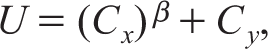
where C_x denotes consumption of the homogeneous good x, C_y denotes consumption of the composite good y consisting of n + 1 varieties and the constant β satisfies 0 < β < 1.

The quasi-linear utility function implies that while the marginal utility of good x is falling, that of good y is constant. This, in turn, ascribes a degree of ‘essentiality’ to good x, its marginal utility being very high for low levels of consumption. But beyond a certain level of consumption, the marginal utility becomes lower than that of the y good and income elasticity becomes zero. Food, produced in the agricultural sector, is a prominent example which fits into this description. It may be noted that for economies like India, which I am trying to model here, agriculture is in the informal sector. So x sector contains the agricultural good. Other traditional manufactures, for which income elasticity is high for low income and low for high income, are also included in the x sector. Sector y, on the other hand, represents modern industrial goods.

Consumption C_y of the composite commodity y is given by the aggregation

C y = [ ∑ i = 0 n λ i 1 − ρ c i ρ ] 1 ρ

(2)

where c_i is consumption of the ith variety good, λ_i > 0 is a parameter representing the relative importance of good i in the commodity basket, and ρ, the elasticity of substitution between two varieties, satisfies 0 < ρ < 1.

At given income and prices, utility is maximized in two stages. In stage 1, the consumer decides how his income is to be divided between consumption of good x and good y so as to maximize Equation (1). In stage 2, he decides how expenditure on good y, as obtained from stage 1 maximization, is to be divided between the different varieties.

I start with stage 2 maximization which involves maximization of Equation (2) by choosing {c_i} subject to

∑ i = 0 n q i c i = I ,

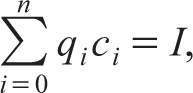
where q_i is the price of the ith variety and I is the expenditure allotted to the purchase of variety goods.

The maximization exercise yields the following demand function for the ith variety good

c i = λ i q i − 1 1 − ρ [ ∑ i = 0 n λ i 1 − ρ c i ρ − 1 ∑ i = 0 n q i ] 1 ρ − 1

(3)

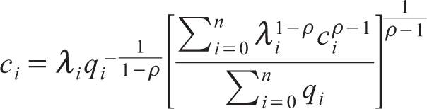
I assume that the number of varieties is large so that a change in q_i keeps the term within the square brackets unchanged. Therefore, own price elasticity of demand for the ith variety good is 1 1 − ρ ≡ σ . Since 0 < ρ < 1, σ > 1. Also,

c i c j = λ i λ j [ q i q j ] − σ

(4)

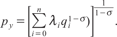
Before I go to the first stage of utility maximization, it is necessary to get an expression for the price of the composite good y. Let p_y be the price of the composite good y. Then, noting that p y = ∑ i = 0 n q i c i and using Equation (4), I get

p y = [ ∑ i = 0 n λ i q i 1 − σ ) ] 1 1 − σ .

(5)

Stage 1 utility maximization involves maximizing Equation (1) subject to the budget constraint

p x C x + p y C y = I ¯ ,

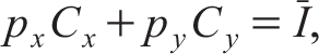
where p_x is the price of the homogeneous good and Ī is total expenditure of the consumer. Assuming that there is no corner solution, ⁴ the maximization exercise yields

p x p y = β ( C x ) β − 1

(6)

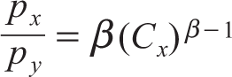
Therefore, consumption of good x is determined by the relative price and the parameter β, which represents the extent of diminishing utility of x, but is independent of the consumption of good y.

A couple of comments are necessary in this context. First, in this model, there are three types of income—formal wage, informal wage and profit, ⁵ which are generated in the formal sector. I assume that a subset of workers employed in the formal sector have ownership of formal sector firms, and, hence, profits are distributed between them.

It follows from the quasi-linear utility function that each type of income earner must necessarily consume the homogeneous good. But to make the model workable, all consumers must consume the variety goods as well, that is, there cannot be a corner solution for any consumer. To see why, let us suppose the contrary that informal sector workers consume only the homogeneous good. But in that case, they do not sell any homogeneous good because they do not have any demand for variety goods (see footnote 5). This, in turn, implies that formal sector workers do not consume any homogeneous good which is not possible because of the quasi-linear utility function. If informal sector workers consume some composite good, the more affluent formal sector workers must necessarily do so. Second, from Equation (6), it is clear that all consumers, irrespective of income, must consume the same amount of good x. It is the level of consumption of the variety goods where consumers will differ.

Let me now turn to the production side. Production of each unit of variety good requires α units of labour, while production of one unit of homogeneous good requires one unit of labour. Since the homogeneous good is produced under perfect competition, in equilibrium, price must be equal to average cost, that is,

p x = w .

(7)

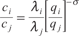
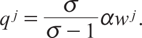
Variety goods, on the other hand, are produced under monopolistic competition, so that profit maximization in each variety good yields

q i = σ σ − 1 α μ w .

(8)

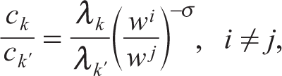
Since the right-hand side of Equation (7) is independent of i, price of each variety good must be the same. I denote this price by q. Again, q_i = q_j implies from Equation (4) that

c i c j = λ i λ j

(9)

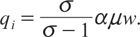
Similarly, using q_i = q_j, Equation (5) yields

p y = q λ 1 1 − σ

(10)

where λ = ∑ i = 0 n λ i .

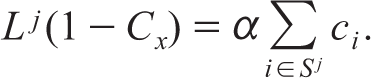
Using Equations (6), (7), (8) and (10), consumption of good x of each consumer can be written as

C x = [ σ λ 1 1 − σ σ − 1 α β μ ] 1 1 − β .

(11)

I assume that initially, that is, before the pandemic, labour is fully employed. ⁶ Since production of each unit of good x requires one unit of labour, total labour requirement in the x sector is LC_x so that labour available for the y sector is L(1 – C_x) ≡ L_y. ⁷

Let c i λ i = γ . Then full employment implies

L y = α ∑ ​ c i = α γ λ ​ .

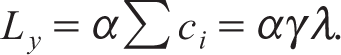
It is then straight-forward to show that

c i = λ i λ L y α = λ i λ L ( 1 − C x ) α

(12)

This completes my description of pre-pandemic equilibrium.

Pandemic and Restrictions on Internal Migration

In a country like India where development is uneven and where labour migrates from the backward to the advanced regions, one of the major problems following the outbreak of the crisis was that of reverse movement of migratory labour to its original place of residence. Restriction on migration was triggered directly by restrictions on free movement of labour across regions and indirectly by lack of transportation, both imposed by the lockdown. Restriction on migration created serious imbalances between demand and supply of labour in each region disrupting production and giving rise to unemployment. To capture the effect of this forced reverse migration due to the pandemic, I divide the economy into m + 1 regions with region j, j = 0, 1, 2, …, m, having L ^j units of units of labour. After the outbreak of the pandemic, labour of each region comes back and remains confined to its original boundaries of residence, that is, there is complete absence of migration. ⁸ To start with, I further assume that the homogeneous good is produced and consumed locally. Therefore, the homogeneous good is perceived to be consisting of services or goods of low value which are not worthwhile to sell in distant regions because the transportation cost involved would be prohibitive, especially due to the pandemic, relative to the value of the good. ⁹ The variety goods, on the other hand, are freely traded across regions, the transportation cost being negligible relative to the value of these goods and, hence, can be ignored. Region j has n ^j firms each producing a different variety. Since there is no labour movement across regions, in each region, the varieties are to be produced with regional labour. To start with, I assume that there is no exit of firms after the pandemic so that ∑n ^j = n.

Since I am looking at the short run, I assume that wage rates in the two sectors temporarily remain unchanged after the pandemic, even if there is unemployment. The wage rates and the number of firms remaining the same, it is straightforward to verify that per capita consumption of x, that is, C_x also remains unchanged. Similarly, relative demand for any two variety goods is given by Equation (9) as before. Let me denote equilibrium variables after the crisis by a ‘tilde’. Then ∀ i

c ˜ i = γ λ ˜ i .

(13)

Clearly, the higher the value of γ ˜ , higher is the value of c ˜ i . Let N ^j be the level of employment in region j after reverse migration. Obviously, N ^j ≤ L ^j. Let S ^j denote the set of varieties produced in region j. Let λ j = ∑ i ∈ S j λ i . Since λ_j subsumes the number of varieties produced in region j as well as their desirability, it is natural to assume that for any two regions j and k, λ ^j > λ^k implies region j is more advanced than region k. Let N x j a n d N y j be employment in sector x and sector y, respectively, in region j. Since each unit of labour employed in the informal sector produces a surplus (over and above its own consumption) of (1 – C_x) to feed formal labour, and since each formal labour consumes C_x units of informal good, I have N y j C x = N x j ( 1 − C x ) . Hence,

N j = N x j + N y j = N y j ( 1 − C x ) = α ( 1 − C x ) ∑ i ∈ S j c ˜ i = α λ j γ ˜ ( 1 − C x ) .

(14)

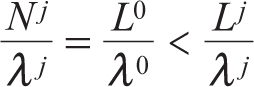
Since N ^j ≤ L ^j, I can write, using Equation (14), ∀ j

γ ˜ ≤ L ​ ​ j λ j 1 − C x α

(15)

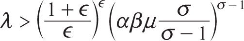
Suppose, without loss of generality, L 0 λ 0 = min { L ​ ​ j λ j } . Also, suppose that the minimum is unique. It is straightforward to see that satisfying Equation (15), γ ˜ reaches its maximum when

γ ˜ = L 0 λ 0 1 − C x α

(16)

This value of γ ˜ maximizes output of each variety, given the no-migration constraint, and in the subsequent analysis, I shall assume this constrained maximum to hold. Therefore, in the equilibrium that follows, output and employment in each region are determined by the parameters of the most labour-constrained region, the region where endowment of labour is minimum relative to the demand for labour. Substituting the value of γ ˜ from Equation (16) in Equations (13) and (14), I get for any region j, j ≠ 0,

N j λ j = L 0 λ 0 < L j λ j

(17)

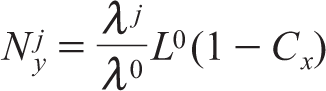
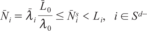
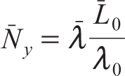
and for any variety good i

c ˜ i = λ i L 0 λ 0 ( 1 − C x ) α

(18)

From Equation (17), it immediately follows that N ^j < L ^j, j ≠ 0, that is except for region 0, total employment goes down in each region. Before the crisis, C_x L ^j of the total labour endowment L ^j of region j was engaged in the informal sector and (1 − C_x)L ^j in the formal sector, though not necessarily in the formal sector of region j itself. After the crisis, the employment levels in the informal and formal sectors go down to N ^jC_x and N ^j(1 − C_x), respectively.

Moreover, I may write

L λ = ∑ ​ L ​ j λ j λ j ∑ ​ λ j > L 0 λ 0 .

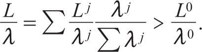
The first equality says that L λ may be expressed as a weighted average of { L ​ j λ j } , and the last inequality follows from the fact that a weighted average of { L ​ ​ j λ ​ ​ j } must be greater than the minimum of { L ​ ​ j λ j } . Therefore, comparing Equation (12) with Equation (18), I can conclude c ˜ i < c i ​ .

The following proposition is immediate.

Proposition 1. When migration of labour across regions is totally restricted, in region j, j = 1, 2, …, m, j ≠ 0 some labour remains unemployed and the extent of unemployment is increasing in { L ​ j λ j } . In each of these regions, both formal and informal employment goes down. Also, production and consumption of all variety goods, including those produced in region 0, go down in the post-pandemic equilibrium.

Employment in the formal sector is structural, while employment in the informal sector is demand-driven. In any region, informal employment is proportional to formal sector employment. ¹⁰ Consider any region j ≠ 0. Employment in the formal sector of this region is

N y j = α λ j γ ˜ .

Higher number of firms operating in region j and higher valuation of consumers of the varieties produced in region j (i.e., higher values of λ i , i ∈ S j ) contribute to a higher value of λ ^j . A higher value of λ ^j , in turn, leads to a higher level of employment in the formal sector of region j. So regional employment in the formal sector depends on the strength of the regional formal sector in terms of number of varieties and desirability of those varieties. But formal employment in region j also depends on the value of γ ˜ which, in turn, is determined by the most labour constrained region, that is, the region which has minimum labour relative to the size of its formal sector. The size of the formal sector in region j, λ ^j , depends upon the number of varieties produced in that region as well as the preferences of the consumers towards these varieties. Given that prices of varieties are constant in the short run, varieties are consumed in fixed proportions. Hence, varieties which are most constrained by labour supply determine output and employment in the other regions. In this sense, unemployment in the formal sector is structural.

To understand further the intuition behind the nature of unemployment, suppose λ_i = 1 for all i. Then, in equilibrium, c ˜ i = c ˜ j = c for all i, j. Formal employment in the jth region is αn ^jc which cannot exceed L ^j (1 – C_x). Clearly, the common consumption c is determined by that region where L ​ ​ j n j is the minimum. This is the maximum c that can be produced satisfying the labour constraint in each region. For the region where L ​ ​ j n j is minimum, labour will be fully employed and for all other regions some unemployment will prevail. This unemployment is partly due to restrictions on labour movement and partly due to the fact that prices are not adjusting in the short run.

Next consider the informal sector. Since each unit of employed labour in the formal sector demands C_x units of informal good and since to produce one unit of surplus of the x good (net of consumption of x good of labour which produces it) 1 1 − C x of labour needs to be employed in the informal sector, informal employment in region j is given by

N x j = N y j C x 1 − C x .

Clearly, employment in the informal sector is driven by employment in the formal sector. Adding N y j and N x j I get total employment

N j = α λ j γ ˜ 1 − C x ,

which is nothing but Equation (14). Here, α λ j γ ˜ can be interpreted as the autonomous part of demand for labour and the term 1 1 − C x as the employment multiplier. ¹¹

It is necessary to delve further into the comparison of the no- migration equilibrium with migration equilibrium. From Equation (12), it is straight-forward to see that in region j, total formal employment in migration equilibrium is λ j λ L ( 1 − C x ) and, hence, informal employment is λ j λ L C x so that total employment is λ j λ L . If λ j λ L > L ​ j , there is migration into region j and if the inequality is reversed, there is migration out of region j. Suppose region j was a net receiver of labour before the pandemic broke out. It experienced a supply shock when migrants went back to their respective regions. If this were the only shock, it could have employed L ^j(1 − C_x) of its labour in its formal sector and L ^jC_x of its labour in the informal sector. But if it does that, it will be producing λ i λ j L j ( 1 − C x ) α units of the ith variety good, i ∈ S ^j. This is less than what it was producing before the pandemic, as is clear from Equation (12). This indicates a supply constraint. But in the post- pandemic situation, if the supply constrained output is produced, it will exceed demand which is given by Equation (18). This means that regions which received net inflow of labour before the pandemic experience a supply shock as well as a demand shock after the pandemic. The demand shock, however, dominates the supply shock and, hence, emerges as the binding constraint. Only the most supply-constrained region, region 0, produces according to its supply shock, and this generates demand shocks in other regions. On the other hand, regions which were net exporters of labour before the pandemic face excess supply in the labour market after the migrants come back. This situation of excess supply is further aggravated by the demand shock generated by production in region 0. To summarize, supply shock in region 0 generate constraining demand shocks in all other regions.

It is worthwhile to make a few observations at this point. First, the informal wage w is fixed by the choice of numeraire and, therefore, unemployment in this model does not depend upon the rigidity of this nominal wage. Suppose, due to unemployment, there is a fall in the nominal wages in the two sectors, keeping the relative wage μ constant. This will lead to proportionate fall in nominal prices of all goods, keeping real output and employment unchanged.

Second, suppose there is a fall in μ, indicating a fall in the relative wage of the formal sector. This can happen if the unions controlling the formal labour market yield to the pressure of unemployment and agree to reduce the formal wage rate. Now, if μ uniformly falls in all regions, this can happen if the same unions control the entire labour market of the country, the relative prices of the varieties remain unchanged keeping formal employment unaffected. The only change in this case takes place in the value of C_X, which falls, leading to a fall in the value of the multiplier and a fall in informal employment as well as total employment. These two observations can be summarized in the following proposition.

Proposition 2. A proportionate fall in the nominal wage in the formal and informal sector keeps real output and employment in each sector unchanged. A fall in the relative wage of the formal sector keeps formal employment and output unchanged, but reduces informal employment and, hence, total employment. ¹²

Third, suppose, production of each variety good involves a fixed cost, in addition to the variable cost. To keep the model simple, suppose β units of ‘skilled’ labour, the cost of which is βw_s, are required to produce each variety. The skilled wage w_s is different from the wage paid to ordinary labour. w_s is rigid and some skilled labour possibly remains unemployed at this wage. ¹³

Now, before the pandemic, gross profit of the ith variety producing firm was given by

π i = μ w λ i σ − 1 L ( 1 − C x ) λ

Similarly post-pandemic gross profit of the ith firm is given by

π ˜ i = μ w λ i σ − 1 L 0 ( 1 − C x ) λ 0

This, in turn, implies that π ˜ i < π i , that is, gross profit of each firm goes down after the pandemic. Net profit is obtained by subtracting fixed cost β w_s from gross profits. I assume that before the pandemic, each firm was making non-negative net profits. After the pandemic, fixed costs remaining the same, gross profit falls for each firm leading to a fall in net profit. For those with low values of λⁱ, it can become negative. These firms will exit the market. Hence, λ ^j will fall. Suppose in each region, λ ^j falls by the same proportion, that is, weaker firms are evenly distributed across regions. Now,

N y j = λ j λ 0 L 0 ( 1 − C x )

and

N j = λ j λ 0 L 0 .

Fall in λ ^j implies a fall in λ. From Equation (11), this leads to a rise in C_x. The ratio λ j λ 0 remaining constant, the rise in C_x leads to a fall in N y j . However, total employment in each region remains constant. All this is summarized in the following proposition.

Proposition 3. Restrictions on migration due to pandemic forces some firms to exit. Assuming that the proportion of firms going out of business is the same for each region, exit of firms increases the degree of informalization of each region, keeping total employment constant.

A fourth question arises as to what extent non-tradability of good x is responsible for the unemployment caused by the lack of labour mobility. A well-known result in trade theory states that free movements of factors can be substituted by free movements of commodities across regions or countries. ¹⁴ So, in the present context, I investigate if pre-pandemic employment with labour mobility can be restored if informal sector goods are tradable.

If the pre-pandemic level of each variety good is to be produced, from Equation (12) the labour requirement in region j is λ j λ L ( 1 − C x ) . So, if this requirement does not exceed L^j, the total labour available in the region, ∀ j ​ then certainly pre-pandemic levels of variety goods can be produced in the economy as a whole. Since L 0 λ 0 = min { L ​ j λ j } , the requirement boils down to

L 0 λ 0 ≥ L λ ( 1 − C x ) .

(19)

If the condition given in Equation (19) is satisfied and good x is fully traded, then in each region, the residual labour after production of variety goods can be allocated to the production of good x. The region where λ^j is small relative to L ^j will produce more x than it consumes and export the excess x to other regions where λ ^j is large relative to L ^j. It is straightforward to see that production of good x in the economy will also be equal to its pre-pandemic level.

What happens if good x is fully traded but the condition given in Equation (19) is not satisfied? ¹⁵ Let c ′ i denote production and consumption of ith variety good in this case. Let γ ′ = c ′ i λ i Then, feasibility requires that in each region j,

α ∑ i ∈ S j c i = α λ ​ γ ′ ≤ L ​ j ​ .

From this, I get

γ ′ = L 0 λ 0 1 α

Accordingly, production and consumption of the ith variety good is given by

c ′ i = λ i L 0 λ 0 1 α

(20)

Comparing Equation (20) with Equation (18), it immediately follows that c ′ i > c ˜ i .

Again total formal employment in the country is given by λ λ 0 L 0 and that in the informal sector by C x 1 − C x λ λ 0 L 0 . Hence, total employment in the country is given by

λ λ 0 L 0 1 − C x < L .

The inequality holds in view of the fact that the condition given in Equation (19) is not satisfied. Since c ′ i > c ˜ i and since employment in sector x is proportional to that in y, total employment increases when good x becomes traded. I summarize my findings in the following proposition.

Proposition 4. With no migration of labour but both goods traded across regions, employment and output goes up in comparison with the situation where there is no migration of labour and only variety goods are traded. Tradability of good x along with that of y can restore pre- pandemic equilibrium if Equation (19) is satisfied, otherwise employment and output remain below the pre-pandemic levels.

A couple of comments are in order. First, though theoretically tradability of goods produced in the informal sector can restore partly or fully the pre-pandemic equilibrium, in practice, some informal sector goods are not tradable. Services constitute one such example. Some other goods are of very low value so that transportation costs prohibit their movements across regions. Second, when informal goods are tradable and Equation (19) is not satisfied, regional employment is indeterminate. Formal sector employment is, of course, determinate being equal to λ j L 0 λ 0 in region j. Indeterminacy arises in the employment of the informal sector. While total informal employment in the country is determinate, how this employment is distributed across regions remains indeterminate.

I end this section by pointing out that the equilibrium described above entails fixed money wages and, hence, fixed nominal prices. In the short run, this seems to be an appropriate assumption. In the medium run, however, nominal wages and prices may go up. This is, of course, consistent with the assumption of downward rigidity of these variables. Now, with upward flexibility, prices can increase by different magnitudes in different regions depending on the varied degrees of labour scarcity of the regions. This, in turn, can lead to changes in relative prices which are consistent with both full employment and consumer equilibrium. I explore such equilibria in the fifth section and argue that they can be achieved through government policies of increasing the liquidity of the economy.

Demand Shocks, Supply Shocks and Unemployment

Economists have recognized that the shock due to the present pandemic is unique in the sense that it cannot be identified exclusively as a supply-side shock or as a demand-side shock. Instead it is a combination of both. Some sectors are directly hit by a demand shock. Consumers are either unable or hesitant to consume the goods produced in these sectors because of lockdown or because of fear of infection. Hotels, restaurants, tourism and entertainment are examples of directly demand-hit sectors. On the other hand, there are sectors which are hit from the supply side. Supply-side shocks may be triggered by a number of factors. Lockdown may directly affect raw materials and labour supplies. Social distancing and work from home may make much of the existing labour force unusable. Willingness to work may reduce the effective labour supply. Again, there could be some sectors which are neither directly affected by demand nor by supply. These sectors may experience spillover effects from shocks to other sectors. In this section, I demonstrate how supply shocks in one sector can cause demand shocks in other sectors.

In this section, I assume away the problem of labour migration. Instead, I focus my attention on supply shocks and demand shocks and their possible spillovers. For the purpose of this section, variety i has to be interpreted as a group of subvarieties. Thus, for any variety i, λ_i = ∑ _j λ _ij where λ_ij are subvarieties within variety i. The reason for interpreting variety i as a group rather than a single product is the following. If variety i is interpreted as a single product, then any demand or supply shock to this product will be negligible as far as the rest of the economy is concerned. If, on the other hand, variety i is interpreted as a group of products, then a shock to this group is likely to have spillover effects elsewhere. ¹⁶

Formal sector firms are divided into different groups: firms directly experiencing negative supply shocks, comprising of a set S ^s; firms directly experiencing negative demand shocks, comprising of a set S ^d–; firms directly experiencing positive demand shocks, comprising of a set S ^d+, and firms, comprising of a set S ⁰, which experience neither a demand nor a supply shock directly, but are open to spillover effects from other sectors. No firm receives a positive supply shock during the pandemic. To understand the separate impacts of demand and supply shocks, I assume, to start with, S ^s ∩ [S ^{d– ∩} S ^d+] = ϕ, which implies that goods having a demand shock are distinct from goods having a supply shock, that is, there is no good which receives both a demand and a supply shock simultaneously. Later, I shall discuss the implications of relaxing this assumption.

First I consider demand shocks only. During the pandemic, some sectors—such as hotels and restaurants tourism and entertainment—received negative demand shocks, while some others—such as software industry, online business, hospitals and medical supplies—received positive demand shocks. There is yet another category of industries which received neither a directly negative nor a directly positive demand shock. In terms of our model, demand shock on good i is captured by a change in λ_i. It can be positive, negative or zero entailing a fall, rise or no change in λ_i. Hence, for i ∈ S ^d–, λ_i goes down and for i ∉ S ^d–, λ_i goes up or remains constant. Let the new values of λ_i be denoted by λ ¯ i where λ ¯ i < λ i for i ∈ S ^d and λ ¯ i ≥ λ i for i ∉ S ^d. We assume, however, that there is a fall in the aggregate value of λ. ¹⁷ Let the new value of λ be denoted by λ ¯ with λ ¯ < λ . From Equation (11), this implies a rise in C_x. Let the new value of C_x be denoted by C ¯ x . Since there is no restriction on employing labour, total employment remains at its pre-pandemic level L, but its distribution between formal and informal sectors changes in favour of the latter and against the former. Let employment in the ith formal good be given by N ¯ i d . Then, I have

N ¯ i d = λ ¯ i λ ¯ L ( 1 − C ¯ x ) .

(21)

From Equation (12), the pre-pandemic level of employment in the ith variety good is given by

L i = λ i λ L ( 1 − C x ) .

(22)

Let ‘hat’ on a variable denote proportionate change. I can write

( 1 − C x ̂ λ ) = ( 1 − C x ̂ ) − λ ̂

From Equation (11), I get

C ̂ x = − 1 ε λ ̂

where ϵ ≡ (1 – β) (σ – 1) > 0. Hence,

( 1 − C x ̂ ) − λ ̂ = [ C x 1 − C x 1 ε − 1 ] λ ̂ .

Clearly, 1 − C x λ goes up as λ goes down provided C x < ε 1 + ε . Since C_x and λ are inversely related, the condition will hold if the number of firms and, hence, λ is sufficiently large. More precisely, I need

λ > ( 1 + ε ε ) ε ( α β μ σ σ − 1 ) σ − 1

(23)

I assume that λ is large enough to satisfy this condition. Consequently, comparing Equation (21) with Equation (22) I can conclude that

Proposition 5. An overall negative demand shock (without a supply shock) increases total informal employment and reduces total formal employment, keeping total employment unchanged. Also, for λ sufficiently large, employment unambiguously increases in varieties with positive or no demand shock, while change in employment in varieties with a negative demand shock is generally ambiguous. However, since total formal employment goes down, some varieties with a negative demand shock must register a fall in employment.

The proposition illustrates that the pandemic can have a differential impact on different sectors with some sectors gaining and some losing. An aggregate demand shock, however, reduces overall formal employment and, hence, is detrimental to the formal sector as a whole. Also total employment remains unchanged. As I shall show below, the situation turns out to be quite different when negative demand shocks are combined with negative supply shocks.

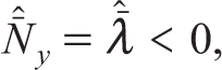
Now consider supply shocks. In the present context, supply shocks take the form of labour shortages. In particular, labour available for employment in variety i is L ¯ i ≤ L i , where L_i is employment in sector i before the pandemic as given by Equation (22) and where strict inequality holds for i ∈ S ^s. A number of justification can be given for this specification. First, for the supply constrained varieties, some existing labour cannot come to the place of work due to lockdown. Second, in these firms, unemployed labour from outside cannot be used because a minimum training is required to make labour suitable for production, and this training cannot be imparted in the short run. ¹⁸ Third, social distancing forces these firms to scale down production and employment.

Let me first consider supply shocks without demand shocks. Let c ¯ i s be consumption of ith good in this situation. Let c ¯ i s λ i = γ ¯ s . Then, I have

α c ¯ i s = α γ ¯ s λ i ≤ L ¯ i .

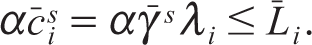
So, γ ¯ s ≤ L ¯ i α λ i and production and employment are maximized by choosing γ ¯ s = L ¯ 0 λ 0 where L ¯ 0 λ 0 = min { L ¯ i λ i } . Hence, employment in the ith sector is given by

N ¯ i s = λ i L ¯ 0 λ 0 .

(24)

Comparison of Equation (24) with Equation (22) immediately yields N ¯ i s < L i .

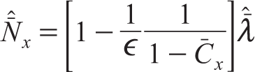
With this, if I add a negative demand shock, I get

N ¯ i = λ ¯ i L ¯ 0 λ 0 ≤ N ¯ i s < L i , i ∈ S d −

(25)

where N ¯ i is employment in ith variety when both negative demand and supply shocks are operating. Clearly, N ¯ i < N ¯ i s for i ∈ S ^s. Aggregate formal employment falls with a negative supply shock and falls further with a negative demand shock when supply constraints are operative.

Employment is partly restored if demand shock is positive. It is clear from the above equation that if λ_i increases, there are two opposing effects on employment. An upward pull on employment is created by an increase in λ_i along with a downward push created by the supply shock. The net effect, however, cannot increase employment beyond the pre-pandemic level, because, by assumption, L ¯ i ≤ L i with strict inequality holding for some i. Consequently, total formal employment goes down. ¹⁹

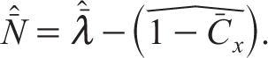
But what happens to informal employment? What happens to total employment? A pure supply shock unambiguously reduces formal employment and since informal employment is proportional to formal employment, informal employment, and therefore total employment, go down as well. But when I add the demand shock, there is an increase in demand for good x through a fall in λ. Let N ¯ x , N ¯ y and N ¯ be informal employment, formal employment and total employment, respectively, after the supply shock. I proceed to find out what happens to these variables after the demand shock. I can write

N ¯ y = λ ¯ L ¯ 0 λ 0

Hence,

N ¯ ̂ y = λ ¯ ̂ < 0 ,

which demonstrates that formal employment falls further after the demand shock. Again, since N ¯ x = C ¯ x 1 − C ¯ x N ¯ y , I can write

N ¯ ̂ x = [ 1 − 1 ε 1 1 − C ¯ x ] λ ¯ ̂

The sign of [ 1 − 1 ε 1 1 − C ¯ x ] is in general ambiguous. It is straight-forward to verify that the expression is positive, negative or zero according as C ¯ x is less than, greater than or equal to ε − 1 ε . Hence, the direction of change in informal employment is ambiguous. However, change in total employment can be written as

N ¯ ̂ = λ ¯ ̂ − ( 1 − C ¯ x ̂ ) .

If Equation (23) holds, the right-hand side is negative. I summarize my findings in the following proposition.

Proposition 6. A supply shock reduces employment in all variety goods as well as that in the informal sector. With supply constraints in place, a demand shock further reduces employment in those variety goods which experience the shock. Total formal employment goes down further, but the direction of change in informal employment is in general ambiguous. However, if λ is sufficiently large, total employment unambiguously goes down further.

I conclude this section with two comments. First, in the preceding analysis, I specifically assumed that demand and supply shocks are confined to the formal sector alone. The informal sector does not receive any direct demand or supply shock. This, of course, does not mean that the informal sector is insulated from the pandemic. In the model, informal activities are dependent on the formal sector and any contraction of the formal sector also affects its informal counterpart. But this is not to deny that the informal sector itself can be directly hit through demand and supply due to the pandemic. But in this article, we abstract away from those direct hits on a number of grounds. First, informal production is usually based on local labour which can travel to its place of work relatively easily during a lockdown compared with formal labour. This reduces the severity of supply shocks to informal production. Again, social distancing rules are less likely to be followed in informal production units which relaxes the constraint on labour use. On the other hand, a large part of informal production consists of agricultural goods which are necessities. Indeed, the quasi linear utility function assumed in this article point to this. Even during a pandemic, these necessities are less prone to demand shocks.

Second, the analysis has assumed that commodities receiving demand shocks are distinct from those receiving supply shocks. In reality, however, a commodity can receive both demand and supply shocks simultaneously. It can be seen, without much difficulty, that the analysis remains unaffected if I allow demand and supply shocks to hit the same commodity, provided the minimum L ˜ 0 λ ˜ 0 remains unaffected. But even if the minimum increases, the basic conclusions remain unchanged if the increase is not extreme.

The preceding analysis assumes fixed nominal wages and prices as is appropriate for the short run. In the medium run, depending on government policies, wages and prices can go up in different proportions leading to equilibria with higher employment. I shall presently explore such equilibria.

Government Intervention

Before I talk about government intervention, I shall demonstrate that it is possible to have an equilibrium with full employment of labour in each region, provided wages are flexible upwards. First, consider the no-migration scenario after the pandemic. I shall describe the equilibrium first and then indicate how it can be attained through appropriate government policy. I continue with the assumption that good x is non-traded. Let w ^j be nominal wage in region j and let q ^j be nominal price of a variety good produced in region j in equilibrium. Then,

q j = σ σ − 1 α w j .

(26)

Informal wage in each region remains pegged at w and, hence, p_x also remains unchanged. p_y is given by Equation (5) and C_x by Equation (6). Finally, relative consumption of two varieties is dependent on their relative price as well as their relative desirability as in Equation (4). Full employment of labour in region j yields

L ​ ​ j ( 1 − C x ) = α ∑ i ∈ S j c i .

(27)

Let k, k' denote two variety goods with k ∈ S ⁱ and k' ∈ S ^j. Using Equations (26) and (4), I can write

c k c k ′ = λ k λ k ′ ( w i w j ) − ​ σ , i ≠ j ,

(28)

and

c k c k ' = λ k λ k ′ , i = j .

(29)

Let L m λ m = max { L j λ j } . Let variety m ′ ​ ​ ​ ∈ S m . Then, for any k ∈ S ^j, j ≠ m, I have from Equation (28)

c k = λ k λ m ′ ( w j w m ) − ​ σ c m ′ .

Similarly from Equation (29), for any i ∈ S ^m,

c i = λ i λ m ′ c m ′ .

These two relationships along with Equation (27) can be used to obtain

L j L m = ∑ k ∈ S j c k ∑ i ∈ S m c i = λ j λ m ( w j w m ) − σ .

(30)

Suppose w^m = μw, that is, in region m, nominal wage remains unchanged. Then from Equation (30), wages in all other regions can be determined. Consequently, prices of all variety goods are also known, and from them output levels can be deduced. Since L m λ m = max { L ​ j λ j } , assuming that the maximum is unique, Equation (30) implies that w ^j > w ^m, and q ^j > q ^m, for all j ≠ m. A bit of reflection will convince the reader that subject to the downward rigidity constraint of money wages and the no-migration condition, the equilibrium described by Equations (26)–(30) delivers full employment with minimum rise in prices. This may be contrasted with the equilibrium described in the third section where output and employment are maximized subject to constant prices.

It may be pointed out that while the equilibrium of the second section, with full labour mobility across regions, is the first best, the equilibrium described by Equations (26)–(30), being a constrained equilibrium with no migration, is a second best. However, it is an improvement over the equilibrium of the third section. There are a number of differences between the unemployment equilibrium described in the third section and the full employment equilibrium described in this section. First, while wage and price in the informal sector is the same in the two equilibria, in the full employment equilibrium, formal wages and prices are higher in all regions but one. Second, economic activity is also higher in the full employment equilibrium than in the unemployment equilibrium because the former makes use of the entire labour force. Third, since in the full employment equilibrium, formal sector prices are higher, the price index p_y is also higher as well. This, in turn, increases C_x as is evident from Equation (6). In other words, in the full employment equilibrium, the size of the informal sector is larger. I shall argue that all these differences increase the demand for money in the economy. If this increased demand is not met, the economy cannot attain the full employment equilibrium. More formally, I postulate

M d = φ ( p x , p y , N , C x ) , φ x > 0 , φ y > 0 , φ N > 0 , φ C x > 0.

(31)

In Equation (31), M ^d is demand for money. It is a function of prices in the two sectors, total employment N (which is a proxy for economic activity) and C_x, the share of labour engaged in the informal sector. I assume that the partial derivatives of ϕ with respect to all four arguments are positive. While it is easy to see why the first three partials are positive, the sign of the last partial derivative needs some explanation. It is implicitly assumed that in the informal sector, transactions are predominantly in cash which is not the case in the formal sector. So much so that an increase in the share of employment in the informal sector increases the demand for money outweighing the negative effect of lower wages in the informal sector on money demand.

It immediately follows from the sign of the derivatives in Equation (31) that demand for liquidity is higher in the full employment equilibrium as compared with the unemployment equilibrium. Now, starting with the unemployment equilibrium, suppose the government makes a series of direct transfers to the unemployed. In each region, the unemployed will spend this transfer on formal goods produced in all regions and informal goods produced in its own region. Due to the increased demand, as long as unemployment prevails in a region, output and employment will increase keeping wages and prices constant. Once full employment is reached in a region, further increase in demand for variety goods coming from other regions will increase wage and prices in the formal sector. Note that no further demand will be created for the informal good and, hence, the informal wage will remain constant. As the government keeps on transferring money to the unemployed, this process will continue, finally converging to the equilibrium described by Equations (26)–(30). ²⁰ I summarize my findings in the following proposition.

Proposition 7. With no interregional migration of labour but upward flexibility of nominal wages and prices in the formal sector, full employment in each region can be achieved through government transfer of money to the unemployed. The full employment equilibrium will involve higher nominal wages and prices.

In a similar manner, government transfer of money to the unemployed may improve the equilibrium of the fourth section. Denoting w ¯ i as the wage rate in ith variety good, ²¹ L ¯ i as the maximum labour available in the production of the ith variety, ∑ ​ L ¯ i = L ¯ , λ ¯ i as the demand parameter corresponding to variety i, ∑ ​ λ ¯ i = λ ¯ and C ¯ x as per capita consumption of good x corresponding to λ ¯ , government transfer can ensure the following second best equilibrium: Employment in the informal sector is L ¯ C ¯ x 1 − C ¯ x , employment in the ith formal good is L ¯ i and

L ¯ i L ¯ m = c ¯ i c ¯ m = λ ¯ i λ ¯ m ( w ¯ i w ¯ m ) − ​ σ

where variety m is that variety for which L ¯ m λ ¯ m is max { L ¯ i λ ¯ i } and w ¯ m = μ w . The details of this equilibrium and how it can be attained are very similar to the equilibrium described by Equations (26)–(30) and, hence, are omitted.

Concluding Remarks

The article built up a simple static general equilibrium framework which can be used to understand effects of a pandemic such as COVID-19 on economic variables such as sectoral and aggregate employment and output. In particular, the framework accommodates an informal sector and interregional migration. These features are specially relevant for less-developed countries like India where development is uneven. I have looked at two major effects of the pandemic: restrictions on interregional migration and constraints on demand and supply of commodities. I show that supply shock in one sector or region generates demand shock in others. While in the existing literature, such effects are shown to be present in an intertemporal framework, the present article shows that they can be obtained in a static set-up as well, provided prices are rigid. It also shows the effectiveness of monetary transfers to improve employment and output. The article is an important step to my future research which aims at developing a fully blown up dynamic stochastic general equilibrium (DSGE) macro model to assess the effects of the pandemic. By introducing many periods, possibly an infinite horizon, into the present model, some basic macro questions can be asked and answered. That is my future research agenda. But even the static model can provide important insights into the pandemic crisis as demonstrated by the present article.