Capital Structure and Risk Preferences

Abstract

This study examined the Korean manufacturing companies listed in the Korea Exchange (KRX) market to see if managerial traits can be one of the determinants of financial structure. This study used the prospect theory definition of risk traits by classifying companies into two groups: risk-averse and risk-seeker. A statistical analysis of the financial structure with several determinants proved that managerial traits play a significant role in determining debt; however, two risk groups did not show different features in determining financial structure. Overall, companies in Korea, except the variable related to size, supported the pecking order theory.

Keywords

Managerial traits financial structure pecking order theory prospect theory Korea

Introduction

Corporate financial structure is a good guide for companies’ financial status. Modigliani and Miller (1958) in their seminal work suggested that corporate financial structure is irrelevant to corporate value. Truly to their suggestions, corporate earnings or cash flow have much to do with corporate value; still, financial structure can be a significant index that leverages high earning variabilities, which may cause serious financial distress to the companies, especially in times of macroeconomic recession. Current economic conditions that cannot comply with neoclassical assumptions of perfect capital market display several factors that have significant influences to the value of the companies caused by financial structure. After the normative model of Modigliani and Miller (1958), many studies in this field were carried out. Of those, the two theories that appear the most in the studies of financial structure are static trade-off theory (hereafter STT) and pecking order theory (hereafter POT). Two theories differ in that the first one tries to figure out an equilibrium status in capital structure, whereas the latter seeks corporate decision-making under asymmetric information. The agency theory explanation stems from STT that views financial structure as a tool to ease conflict between principal and agent (Jensen, 1986).

Studies, thereafter, are focused on the relationship between value and financial structure by easing the strict neoclassical assumptions one by one. Contradicting Modigliani and Miller (1963), some studies proved that tax effect exists that can lead to optimal capital structure (DeAngelo & Masulis, 1980; Scott, 1976). The debt level should be decided cautiously because it influences companies in terms of risk. Financial risk is accompanied with debt level so that tax effect and risk increase can be traded off; therefore, optimal debt level exists to maximise corporate value (Kraus & Litzenberger, 1973). The concept of informational asymmetry was introduced to corporate finance studies. Managers with superior inside information, in need of additional capital to fund investment opportunities, do not share same information quality with external investors. They may demand for higher return to compensate the risk; sometimes a sizeable sum of cost will incur by issuing new securities (Myers & Majluf, 1984).

This study focuses on capital structure of the companies when managers are not always rational and risk-averse. Companies’corporate finance decision-making will be carried out by the management whose risk attitude cannot always be risk-averse. Companies with different managerial traits may demonstrate different financial decisions, hence will likely affect the determinants of financial structure. Managements’ risk attitude was classified into risk-averse and risk-seeker, by using prospect theory. When managements face firm performances less than their target, return will likely become risk-seeker and vice versa (Kahneman & Tversky, 1979). To this intuition, determining their capital structure may change due to managers’ risk attitudes. To test this, this study analyses Korean companies’ financial structure and their determinants. This study used prospect theory to classify companies into two groups by their risk attitudes. Over-performed companies are included in the group of risk-averse and underperformed companies to the risk-seeker group. Managerial risk (Mrisk) attitude is measured by distant-to-target and implemented as one of the determinants of corporate structure.

This result of this study corroborates POT explanations but not fully. The profit of the companies interacted conversely with the leverage that supported POT explanation, but firm size was positively related to the leverage that supported STT explanation as well. Mrisk is an important factor to decide leverage for the over-performed companies that perform more than their target, but not to the companies that underperformed their target. The two groups of the over-performed and underperformed companies showed similar behaviour in deciding their leverage level. This study implemented Mrisk attitude in corporate structure, which proved that Mrisk is a significant factor in determining the degree of leverage.

Prospect theory and Debt Financing: Literature Review

Capital structure is truly a puzzle. How the managers in the field make decision about their financial structure is also a puzzle. It is still quite unknown if managers have certain guideline about the target measure or if their intuition worked to make the financial decision. Graham and Harvey (2001) asserted that in the real-world companies do not follow guidelines from conventional financial textbook when making financial decisions such as capital structure.

Studies related to capital structure support ideas of the two theories suggested above. Empirical studies seek debt structure related to companies’ financial conditions. Capital structure studies, supporting STT, considered companies’ assets as collateral value, whereas profit variabilities can be a risk factor for companies to keep ‘ongoing’ concerns. Similarly, debt usage increases firm value for they have tax shield effects, but can also increase financial risk and impose even higher profit variabilities; so that it explains financial conditions that increase in firm value will likely increase debt as well. Financial risk or default risk measures are determinants that decrease debt. This theory tried to seek equilibrium status of debt within the boundary of a company considering several determinants. The empirical studies have observed determinants such as tangibility, profit, tax shield, non-debt tax shield, profit variability and size of the companies that affect debt structure. Variables that have positive impact on the firm value also have positive impact on debt level. There are determinants that offset the benefits of firm value. POT theory weighs on capital cost of fund introduced to companies incurred by informational asymmetry. To minimise cost of funding, the best choice is to use corporate reserves, then debt and then issuing new securities should be the last means. POT explanation, therefore, focuses on profit, cash holding, size of the firm and investment opportunities. POT neither cares about optimal debt degree nor targets the leverage of a company.

The two theories mentioned above are not mutually exclusive relationship, but are likely to be complementary to each other. STT and POT, both have contributed to corporate finance theories in that they have built theories on the basis of Modigliani and Miller (1958, 1963), which was a normative model from strict neoclassical assumptions of perfect market. The strict neoclassical assumptions they used were eased one by one as the studies in this field were developed; however, the assumption of managers’ traits of being rational and risk-averse is still kept in many studies. Prospect theory suggests that individuals can react in different ways, thus show different risk preferences under different circumstances. Kahneman and Tversky (1979) suggested in their laboratory study that when individuals perform above the target, they will likely show risk-averse attitude, that is, lower risk and lower expected outcome; however, those who perform below the target level will then be risk-seekers. Johnson (1994) used samples of commercial banking industry in the US market. He used risk measures of equation by Fishburn (1977). By statistically analysing between risk measures by distance and variabilities of rate of return, he asserted that below target level companies showed strong statistical relationship between distance-to-target measures and variabilities of rate of return compared to above target level companies. Fiegenbaum (1990) and Fiegenbaum and Thomas (1988) used Bowman’s risk-return measures to support prospect theory. They found negative relationship between risk and return in the under target level companies, but positive relationship between the over-the-target level companies. Prospect theory takes more realistic steps which also go along with the tracks supporting contingent theory in the modern business theory that companies’ decision-makings are affected by business environment. Similarly, Hackbarth (2008) asserted about managerial traits in the view of trade-off model that optimistic managers are overconfident; that they use more debt. He used agency theory to solve the problem and increase firm value according to management attitudes to risk. Cronqvist, Makhija and Yonker (2012) also showed that the CEOs’ behaviours influence corporate financial decision-making significantly. The studies related to management traits can be intuitive and significant; however, the heterogeneity in the CEO’s attitude is so diverse that it is fairly difficult to take everyone’s traits into consideration and make one general explanation. Prospect theory gives good intuition and expectation of management traits under special circumstances.

This study seeks Mrisk traits by grouping companies into higher group and lower group. The earning before interest and tax (EBIT) to total asset ratio is used to measure rate of return. Every year in the sample period EBIT is compared against target measure (reference measure). The target measure is calculated by average of 5 years of EBIT advance to the sample year. When companies over-perform the historical average, then they are grouped to higher group (risk-averse); and when companies underperform then they are grouped to lower group (risk-seeker). Managers in the higher group are assumed to be risk-averse and vice versa. After grouping companies to assume managerial traits, then by cross-sectional analysis this study seeks effects of the determinants of financial structure.

Empirical Methodology

The empirical design of this research takes two steps. First, this study classifies companies into two groups by using respective companies’ performances: higher group and lower group. This procedure defines Mrisk traits of each company used in the sample. Then cross-sectional analysis is undertaken to see the interaction between leverage and capital structure determinants.

Managerial Risk Traits Using Prospect Theory

Kahneman and Tversky (1979) asserted prospect theory by their experimental research that showed that people do not tend to react in a uniform way, but were affected highly by their performances. If they are underperforming then they have propensity to be risk taker but if they are over performing then¹ they can be classified to risk averse. The risk-averse group of the over-performing group utility graph is, therefore, less steeper than the risk-seeker group utility graph of the underperforming group.

Fishburn (1977) defined risk function of distance from the target measures.

R (t) = \int_{- \infty}^{t} {(t - x)}^{2} d F (x),

(1)

where

R(t) = measure of risk;

t = target level;

α= sensitivity to deviation from target, α > 0; and

F(t) = probability density function of x.

The sensitivity measure of α is higher with the risk-seeker group than with that of the risk-averse group. More specifically, 0 < α < 1 means risk is felt relatively not as much as distance-to-target measure. The risk-seeker group may be included in this range. When α > 1, then risk may be measured as quite large compared to distance-to-target. Laughhunn, Payne and Crum (1980), when tested the underperforming companies, found 71 per cent of the managers showed risk-seeking characteristics.

Johnson (1994) used a modified methodology where he set the target measure using median Return on Asset (ROA), Return on Equity (ROE) and Primary Capital Ratio (PCR) of companies in the banking industries. He used industry median of the average measure to make the target ratio more neutral. The measure of risk by distance-to- target of each company, in the sample analysed, demonstrated correlation between distance-to-target and standard deviation of rate of performance measure. Most of the correlation results demonstrated negative correlations, but the underperforming companies demonstrated statistically significant results. They also suggested that ROA and ROE are good measures for the managerial target.

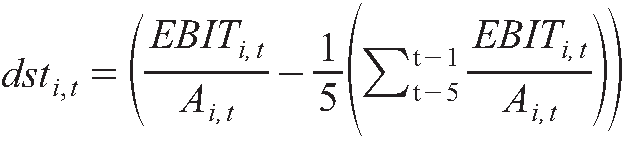
This study modifies Fishburn’s risk equation that was also used by Johnson (1994). Risk is measured by the volatility of profit or rate of return. The distance of profit or rate of return from target rate is the managers’ gain and loss, risk traits. This study used EBIT to asset ratio as the rate of return. The reference measure or target measure used companies’ five years average of EBIT to asset ratio advance to each year. For instance, for calculating risk of i company in year 2005, EBIT from year 2000 to 2004 was averaged. Rather than setting an industrial median or an average figure as target ratio, historical performances of respective companies will make better target figure. Industrial target is also a good standard for companies when making corporate decisions; however, size and life cycle of companies may vary within an industry, therefore may not be a realistic standard for the companies. Rather, five years of company return average may play a better role in company’s decision-making process. The managers’ gain and loss is measured by the difference between companies’ yearly EBIT ratio and target ratio.

d s t_{i, t} = (\frac{E B I T_{i, t}}{A_{i, t}} - \frac{1}{5} (\sum_{t - 5}^{t - 1} \frac{E B I T_{i, t}}{A_{i, t}}))

(2)

where

dst_i,t= distance-to-target of i company in year t;

EBIT_i,t= earning before interest and tax of i company in year t; and

A_i,t = total asset of i company in year t.

The managers’ risk traits are measured by Equation (2) and the performance index of EBIT to asset ratio is regressed statistically to find a relationship between the two. The coefficient of dst (β) will indicate the relationship between risk and return. The analysis of coefficient result has to be carefully done for the higher group; the larger the risk, the better they had performed. In other words, if β = 1 then managers are risk neutral because they require same level of the return out of risk. If β > 1, then it means more risk was driven out of the return; when β < 1, then less risk for the return (risk-averse). Two cases of the higher group and lower group have to be taken into consideration. The coefficient of the higher group will likely show less than 1 and the lower group may have a larger value of coefficient compared to that of the higher group.

R i s k_{i, t} = α + β d s t_{i, t} + ε_{i, t}

(3)

where

Risk_i,t₌ risk of i company in year t (variance of the net income);

dst_i,_t= distance-to-target of i company in year t (by Equation(2));

α = constant; and

ε =error term.

Companies that are performing far well, which are not near the reference point, will then demand less return to risk. Kahneman and Tversky (1979) asserted that value and gain (loss) relation is steeper for losses than gains. Therefore, risk-seekers demonstrate concave function for losses and covex function for gains. To analyse more specifically, this study classifies the higher group to high higher group (HH) and low higher group (LH). The lower group is also classified to high lower group (HL) and low lower group (LL).

After the regression of Equation (3), risk term is post-estimated and then is implemented to the capital structure determinants model as Mrisk.

Leverage Determinant Model and Expectation of the Variables

This test is to see what factor or determinant affects debt and in which way. The purpose of the test is to see if the managerial traits corroborate different theories of corporate structure: STT and POT. The dependent variable is debt to total asset ratio, leverage. Book value of the debt ratio is used in this study. Managers and creditors are more interested in the book value of the debt ratio when using or lending fund to a company. In addition most of the empirical analysis showed obvious results when using book leverage (Fama & French, 2002).

Cash holding is high for the firms that will tend to borrow less according to POT explanation. Companies holding large sum of cash will not be a profitable decision, but can counteract instantly in the need of emergency fund. Cash holding may not affect much in the collateral side of company value, but company may not reach out to debt with abundant cash in house. Cash holding is expected to show inverse relationship with debt ratio(De Miguel & Pindado, 2001). In this study cash and equivalent is divided by total asset.

Tangibility is the term that adds to corporate value. It is also a good index of corporate collateral. This term will not confuse outside fund supplier who are usually distracted by informational asymmetry of being positioned in the outside of the companies. Tangibility is calculated by corporate fixed assets divided by total asset. The expected relationship between tangibility ratio and debt ratio is positive. So that when tangibility increases the debt ratio has propensity to increase as well.

Free cash flow is excess cash flow from the asset that can be distributed to creditors and stockholders (Ross, Westerfield, Jordan, Wong, & Wong, 2015). Jensen (1986) asserted that managerial exploitation will increase as free cash flow increases and that conflict between shareholders and managers can be mediated introducing external fund such as debt to control manager’s discretion. Interaction between free cash flow ratio and debt ratio is positive in agency explanation, moreover STT explanation. POT explanation leads to inverse relationship between the two. Companies with free cash flow will have less incentive to borrow from outside. Companies with large investment opportunities may have different decision on free cash flow. Companies with more investment do not need a control factor for the conflict because they will likely use the fund when they have new investment opportunities (Fama & French, 2002; Jensen & Meckling, 1976).

Profitability is company performance index. This shows how that company has performed throughout the respec tive financial years. STT explains that firms with high profit increase firm value, therefore debt ratio increases; however, POT explains that more profitable firm will likely possess more corporate reserves, therefore will likely use less debt. Profitability is calculated as net income divided by total asset.

Size of the firm is calculated by natural log over total asset. This term also indicates converse interaction with leverage. STT asserts that size of the firm has positive relationship because the larger the size of a firm, the less probability of a company being bankrupt and a high possibility of higher value. But by the POT explanation, the smaller the size of the company, the larger will be the information asymmetry between insider and outsider. Therefore, smaller companies will have less chance of direct financing, which is usually issuing stock in the capital market that companies will rather lean on the debt financing. Therefore, by the STT explanation size and debt ratio is positively related, but by POT it is inverse relationship.

Profit variability is used as risk of a firm. Usually, by the interaction between debt determinants and leverage, stability of profit is implicitly assumed. High profit variance affects diverse areas of companies’ operational system; hence, financial decision will be quite limited according to the variance. Profit variance is risk to companies. Risk has negative impact on firm value that will induce less debt. Risk increases cost of capital; therefore, companies decreasing outside fund will result in less debt by POT explanation. The profit variance is calculated by standard deviation of profit (Balakrishnan & Fox, 1993).

The risk of a manager is calculated by Equation (3). Will the companies react differently according to the managers’ risk? Risk has inverse interaction with debt ratio. However, managerial subject risk may demonstrate different results. When a manager is risk-averse he or she shall try to reduce debt, but if the manager is risk-seeker he or she will use even more funds to invest in risky assets. In this study, the Mrisk is measured by the distance-to-target. Therefore, in the higher group, high figures mean high performances. By STT the interaction would be expected to be positive, but by POT the interaction would be inverse. In the lower group, high figures mean low performances; that is, by STT inverse relationship and by POT positive relationship is expected.

Investment is measured by growth in assets divided by total asset. POT asserts firms need more fund if company has investment opportunities; therefore, the interaction between investment and debt ratio would be positive. STT explanation for investment opportunities and debt relations is not direct. STT borrows agency explanation of controlling factor to ease conflict between management and shareholders and between bondholder and shareholder, in case of under investment (Jensen, 1986). According to STT, the relationship between investment and debt ratio is inverse.

Non-debt tax shield (NDTS) is a substitute for debt tax shield. DeAngelo and Masulis (1980) asserted in their study that R&D expenditure and depreciation are the good source for the tax deduction. They explained that non-debt tax reducing sources can be a substitution for debt so the debt ratio and this variable show inverse interaction. However, companies with high profit may enjoy high tax reduction, thus increases the firm value to increase debt ratio. Companies that demonstrated loss in the financial year may not be able to see any benefits of NDTS. Therefore, companies that are underperforming may not show statistically significant results.

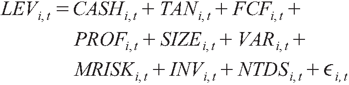
The model to test effects of determinants of the capital structure is shown in Equation (4).

\begin{matrix} L E V_{i, t} = C A S H_{i, t} + T A N_{i, t} + F C F_{i, t} + \\ P R O F_{i, t} + S I Z E_{i, t} + V A R_{i, t} + \\ M R I S K_{i, t} + I N V_{i, t} + N T D S_{i, t} + ε_{i, t} \end{matrix}

(4)

where,

LEV_i,t= total debt/total asset of i company in period t

CASH_i,t = cash and equivalent/total asset of i company in period t

TAN_i,t = fixed asset/total asset of i company in period t

FCF_i,t = (total cash inflow–total investment) of i company in period t²

PROF_i,t = net income/total asset of i company in period t

SIZE_i,t = Ln(total asset) of i company in period t

VAR_i,t = Standard deviation (net income) of i company in period t

MRISK_i,t = post-estimation of Mrisk by Equation (3) of i company in period t

INV_i,t= (fixed asset_i,t–fixed asset _i,t-1)/total asset of i company in period t

NTDS_i,t = depreciation/total asset i company in period t

Empirical test Result

Data and Simple Statistics

The data used in this study were gathered from Korea Information Service-VALUE (KIS-VALUE) files in Korea. Financial firms and utility firms were excluded. Publicly traded manufacturing firms in Korea Exchange (KRX) market from 2005 to 2014 were analysed. The finally selected firms in the sample fulfil the condition of continuously operating firm during the sample period.

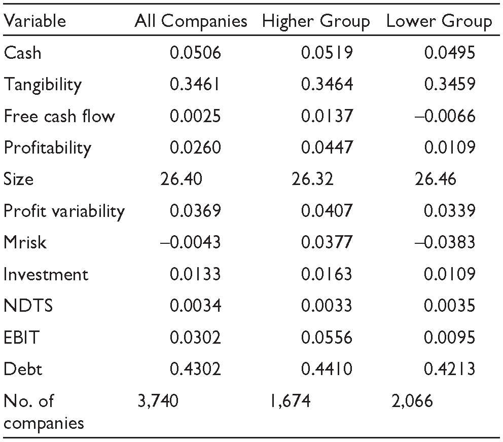
Simple statistics of the variables used in this study are summarised in Table 1. Except the variable tangibility and NDTS, two groups differ in the numbers of respective variables. T-test of mean comparison was undertaken and was proved to be statistically different in their numbers, except tangibility and NDTS. The higher group showed higher values in cash holdings, free cash flow, profitability, Mrisk and investment. However, size of the companies was not larger than that of the companies in the lower group. Mrisk was smaller than the lower group; hence, lower group risk is higher than that of the higher group on an average. For the pooled data Odinary Least Square (OLS), correlation test proved variables are not correlated closely enough, that is, multicollinearity problem will not affect regression result.

Table 1.

Summary of Statistics

Variable	All Companies	Higher Group	Lower Group
Cash	0.0506	0.0519	0.0495
Tangibility	0.3461	0.3464	0.3459
Free cash flow	0.0025	0.0137	–0.0066
Profitability	0.0260	0.0447	0.0109
Size	26.40	26.32	26.46
Profit variability	0.0369	0.0407	0.0339
Mrisk	–0.0043	0.0377	–0.0383
Investment	0.0133	0.0163	0.0109
NDTS	0.0034	0.0033	0.0035
EBIT	0.0302	0.0556	0.0095
Debt	0.4302	0.4410	0.4213
No. of companies	3,740	1,674	2,066

Sources: Author’s statistical results by using STATA13.0 (Statistic software). The financial data were provided by KIS-VALUE.

Regression Result of Risk and Return

Mrisk traits are tested by regression analysis which is summarised in Table 2. In the result table, all the figures are statistically significant and the explanatory power of the regression model is strong. Two groups demonstrated coefficient (β) value less than 1. β in the lower group is –0.5096 and 0.7433 in the higher group. The coefficient of the lower group is negative which coincides results of Fiegenbaum and Thomas (1986) and Johnson (1994). But this does not corroborates prospect theory approach about less sensitiveness of the risk to return in the higher group than the lower group.

Table 2.

Regression on Risk and Return to Find Managerial Risk Traits

Independent Variable	All Companies	Higher Group	Lower Group
dst	0.0806 (7.40)***	0.7433 (49.40)***	–0.5096 (–55.04)***
Constant	0.0373 (51.86)***	0.0127 (12.67)***	0.0144 (23.74)***
R-squared	0.0142	0.5931	0.5946
No. of companies	3,740	1,674	2,066

Sources: Author’s statistical results by using STATA13.0 (Statistic software). The financial data were provided by KIS-VALUE.

Notes: *** 1 per cent significant level, ** 5 per cent significant level and * 10 per cent significant level. The regression of the risk and gain (loss; by dst) of all companies in the sample period from 2005 to 2014; according to the level of distant-to-target measure (dst), companies are classified into two groups: higher group and lower group. The higher group companies over-performed the target measure and the lower group companies underperformed the target measure.

To see the behaviour of the companies more meticulously, this study split companies more narrowly to quartile before executing the same regression analysis as above. Companies are classified into two subgroups again in each group: HH, LH, HL, LL. The regression result is summarised in Table 3. The overall result is not different with Table 2 as the higher group is more sensitive to risk than the lower group. All the figures in Table 3 are statistically significant. However, groups such as LH and HL show meek relationship between return and risk. LH, which is positioned in the higher group, demonstrates higher value than that of the lower group, HL. Companies positioned near target points show different aspects. Statistical explanatory power is also low. The coefficient of HH, 0.7745 is lower than that of LL, –0.5346. In this regression analysis, LL shows the most statistical explanation power (R²). It can be read that companies which demonstrate high gains and low losses represent the behavioural traits of each group than companies whose return are near the target measures.

Table 3.

Regression Analysis of Risk and Return to Find Managerial Risk Traits; Quartile Classification

Independent Variable	Higher Group		Lower Group
	HH	LH	HL	LL
Dst	0.7745 (34.36)***	0.3474 (3.99)***	–0.1829 (–2.42)***	–0.5346 (–42.26)***
Constant	0.0084 (4.00)***	0.0193 (17.00)***	0.0197 (19.38)***	0.0111 (9.63)***
R-squared(adj)	0.5852	0.0175	0.0047	0.6332
No. of companies	837	837	1,031	1,035

Sources: Author’s statistical results by using STATA13.0 (Statistic software). The financial data were provided by KIS-VALUE.

Notes: *** 1 per cent significant level, ** 5 per cent significant level and * 10 per cent significant level. The regression of the risk and return of all companies in the sample period from 2005 to 2014; according to the level of distant-to-target measure (dst), companies are classified into two groups; higher group and lower group. The higher group companies over-performed the target measure and the lower group companies underperformed the target measure. This analysis classified companies in the sample into four quartile: HH, LH, HL and LL.

Figure 1 shows the relationship between risk and return. The higher group shows steeper slope compared to that of the lower group. This value function does not corroborate prospect theory assertion of behaviour of managers in gain and losses.

Figure 1.

Source: Author’s drawing using STATA13.0 (Statistic software) using result from Table 2.

Regression Result of Leverage Determinants

The pooled data OLS regression analysis result is summarised in Table 4. This table indicates all the companies in the sample period regression result and also the higher group and lower group results are summarised here.

All the companies, including the higher and lower group, supported POT. But to some degree, they also support STT as well. All the figures and signs in the table show a similar result. To POT explanation debt has converse relationship with cash holdings. Tangibility, that is, direct collateral to firm is increasing function with debt ratio. This is also true with STT. Free Cash Flow (FCF), if used as to mitigate conflict should show positive relationship, but displays negative sign. These results mean companies use free cash flow for debt repayment or other corporate financial expenses rather than political issues. Profitability has inverse relationship with debt ratio. This result strongly supports POT. Companies use their internally collected fund to minimise capital cost (Fama & French, 2002; Graham & Harvey, 2001; Rajan & Zingales, 1995). The over-performed companies in the higher group employ more debt than the lower group, seeing that with the 1 per cent increase in the profitability the higher group reduced 0.5575 per cent of debt where the lower group reduced 0.9216 per cent. The result on size variable does not support POT; it supports STT. The higher group’s coefficient size is 0.0246, but the lower group companies show 0.0167 coefficient size. Companies increase debt as their size increases, but this is more sensitive on the higher group.

Risk and leverage relationship is the same with the higher and lower group. Both the groups are analysed to increase debt as risk increases. Both the groups’ coefficients of the profit variability are positive and statistically significant. These relationships do not concede with conventional theory explanation of STT and POT. The recent trend of using less debt in the Korean companies resulted that companies with high risk used more debt than the lower risk companies.

Mrisk traits are positively related with debt in the higher group but negatively related in the lower group. Companies in the higher group are more sensitive about their profit volatilities, but the coefficient did not prove to be statistically significant. Companies in the higher group tend to increase debt as the distance-to-target increases, which is usually more profit compared to past average. As to companies in the lower group, the coefficient is negative and statistically significant. This means that as their distance-to-target (dst) increases, which is larger profit loss compared to their previous average, they still increase their debt from outside.

Investment opportunity is inversely related to debt. This result supports STT. But to take a closer look at the figures of the lower group, they lack statistical significance. Only the higher group figures are statistically significant with a negative sign. POT explanation asserts, companies that have enough internal reserve will not use debt when they encounter investment opportunities. The higher group that performed well in the sample period may possess internal reserve enough to borrow funds from outside for investment opportunities. Going back to Table 1 of simple statistics of variables, lower companies invest as much as higher companies do, but investment is not the factor that affects the leverage level. Lastly, NDTS is only statistically significant in the higher group companies. Companies not performing well do not bother to seek tax shield, therefore show non-significant results in other groups. Only the higher group that shows negative relationship supports the idea of DeAngelo and Masulis (1980) of substitution theory of debt. It shows quite a strong inverse relation with debt ratio (De Miguel & Pindado, 2001).

Table 5 summarises four subgroups’ regression result. The interaction between respective variables and debt ratio are overall similar with Table 4. Debt ratio of two groups, near-the-target groups, is affected more by a slight change in the independent variables such as profit variability, Mrisk and size. The HL group demonstrates –1.3065%) of change in debt ratio as the profitability change by 1% and (–7.1589%)of change in debt ratio when Mrisk change by 1%. However, investment and NDTS variables inter acted to debt ratio with no statistical significance. In fact, NDTS only had statistical significance with the HH group. Companies with large profits need NDTS for their value increase. Other groups may not need to consider this problem as they did not achieve enough to avoid tax expenses.

Table 4.

Regression of Determinants of Leverage

Independent Variable	All Companies	Higher Group	Lower Group
Cash	–0.5574 (–10.34)***	–0.4637 (–6.28)***	–0.5999 (–8.28)***
Tangibility	0.1853 (9.96)***	0.1680 (6.13)***	0.1867 (7.51)***
Free cash flow	–0.1416 (–4.86)***	–0.1468 (–3.36)***	–0.1585 (–4.02)***
Profitability	–0.6399 (–19.38)***	–0.5775 (–12.48)***	–0.9216 (–17.54)***
Size	0.0188 (9.16)***	0.0246 (8.04)***	0.0167 (6.15)***
Profit variability	0.4588 (4.53)***	0.4492 (3.63)***	0.5130 (3.02)***
Mrisk	0.1216 (0.94)	0.2504 (1.58)	–0.7050 (–3.07)***
Investment	–0.0991 (–2.74)***	–0.1872 (–3.33)***	–0.0507 (–1.05)
NDTS	–0.6726 (–1.61)	–0.9389 (–1.69)*	–0.0881 (–0.14)
R-squared(adj)	0.2208	0.1936	0.2762
No. of companies	3,716	1,667	2,049

Sources: Author’s statistical results by using STATA13.0 (Statistic software). The financial data were provided by KIS-VALUE.

Notes: *** 1 per cent significant level, ** 5 per cent significant level and * 10 per cent significant level. The regression result of the variables that affect leverage; companies in the sample period from 2005 to 2014 were analysed. According to the level of distant-to-target measure (dst), companies are classified into two groups: higher group and lower group. The higher group companies over-performed the target measure and the lower group companies underperformed the target measure. Mrisk is post-estimated from regression result of Table 2.

Table 5.

Regression of Determinants of Leverage; Quartile Classification

Independent variable	Higher group		Lower Group
	HH	LH	HL	LL
Cash	–0.4863(–4.48)***	–0.4739(–4.16)***	–0.5266(–5.16)***	–0.6352(–6.16)***
Tangibility	0.1466(3.81)***	0.1674(4.25)***	0.1037(2.83)***	0.2370(6.82)***
Free cash flow	–0.1343(–2.37)***	–0.1572(–2.23)**	–0.0890(–1.30)	–0.2159(–4.36)***
Profitability	–0.5254(–9.12)***	–0.6977(–8.84)***	–1.3065(–12.88)***	–0.7657(–12.19)***
Size	0.0183(4.21)***	0.0346(7.96)***	0.0250(6.56)***	0.0086(2.24)**
Profit variability	0.3651(2.70)***	0.9726(3.03)***	0.9577(3.15)***	0.2244(1.08)
Mrisk	0.1552(0.89)	3.5893(1.57)	–7.1589(–1.82)*	–0.2156(–0.78)
Investment	–0.2287(–3.40)***	–0.0608(–0.58)	0.0860(0.98)	–0.1391(–2.01)**
NDTS	–1.6186(–2.13)**	–0.0117(0.01)	1.002(1.36)	–1.5600(–1.37)
R-squared	0.2762	0.2054	0.2507	0.3112
No. of companies	835	832	1,018	1,031

Sources: Author’s statistical results by using STATA13.0 (Statistic software). The financial data were provided by KIS-VALUE.

Notes: The regression result of the variables that affect leverage; companies in the sample period from 2005 to 2014 were analysed. According to the level of distant-to-target measure (dst), companies are classified into two groups: higher group and lower group. The higher group companies over-performed the target measure and the lower group companies underperformed the target measure. This analysis classified companies in the sample into four quartile: HH, LH, HL and LL. Mrisk is post-estimated from the regression result of Table 2.

Companies in the LL group determine leverage not by risk but by investment and cash holdings. Investment opportunity decreased debt ratio by –0.1391. This figure is not as much as the HH figure of –0.2287. Investment interacts conversely with debt but with the HH group it reduced more debt compared to LL. The HH group considers investment opportunity risky and tries to use less debt; rather, they use internal reserves or by issuing new shares. The LL group may not be able to use internal reserve because they have not been performing well to include them nor could they be able to issue a new share which will cost them higher than using debt.

This result confirms that the Korean companies support POT except the result of size variable. The signs of the coefficient were usually similar, except Mrisk, over different groups. The absolute value of coefficients of Mrisk in the lower group is higher than the higher group. This implies that companies in the lower group change debt ratio higher than the companies in the higher group. This, to some degree, corroborates that prospect theory of underperformed companies are more sensitive to losses therefore react sensitively compared to over-performed companies.

Conclusion and Discussions

What are the financial decision-making processes of the companies that confront different economic situations? Do Mrisk traits affect decision-making that lead to leverage decisions? The question was to seek the answer of whether companies in different economic situation make same financial decision or not. Therefore to state the result can be explained by STT or POT. From the empirical test confirmed in this study, it was asserted that the two theories can be complementary to each other rather than being contradictory.

This test, first, classifies companies into two groups of risk-averse and risk-seeker. The prospect theory asserted that individuals may behave differently upon their economic situation of loss and gain. When an individual gains from a certain game he or she tend to become risk-averse, but when an individual loses he or she would become risk-averse, that is, he or she would go into games of high variance. With this intuition, companies are set by the target measure to classify them into two groups of higher group for risk-averse and lower group for risk-seeker. The lower group did not show more sensitiveness between risk and return (gain or loss) relationship compared to the higher group. Companies that performed near the target measure demonstrated meek relationship of risk and return. Most of the companies far from the target measure showed more obvious relationship of risk and return.

POT is more likely to be supported in this study. POT and STT share similar expectation on the determinants of leverage such as profitability that is conversely related to leverage. This relationship tells that companies are relying on the internal reserve rather than finding equilibrium status of debt structure within the company. Except the size, which supported STT of positive interaction with leverage, other variables supported POT expectations. Finally, the risk traits have explanatory power making decision upon leverage. In the underperformed group of risk-seeker, especially in the group of LL, risk did not affect the level of leverage. The HL group showed strong positive relationship with leverage. The risk-averse group of over-performed group showed positive relationship with leverage. The two groups of LH and HL that are near the target point showed higher coefficient of profit and risk variables than the HH and LL groups. These two groups actively react to the risk factor than the HH and LL groups.

Overall, managerial traits have confirmed that financial decision-making can be affected by the risk traits, but could not prove to show that different risk traits support different theory. Due to recent economic down turn, many companies tend to reduce cost, this trend leads to POT explanations reliable in explaining current trend in financial decision making.

This study has contributed in the theory of finance in that assumption of rationality affects capital structure model. It is proved by empirical test that managerial risk trait serve to have impact on the level of leverage. Behavioral finance is a new area to study which will provide better understandings for managers to make financial decisions.

Footnotes

Notes

References

Balakrishnan

, & Fox

(1993). Asset specificity, firm heterogeneity and capital structure. Strategic Management Journal, 14(1), 3–16.

Cronqvist

, Makhija

A.K.

, & Yonker

S.E.

(2012). Behavioral consistency in corporate finance: CEO personal and corporate leverage. Journal of Financial Economics, 103(1), 20–40.

De Miguel

, & Pindado

(2001). Determinants of capital structure: New evidence from Spanish panel data. Journal of Corporate Finance, 7(1), 77–99.

DeAngelo

, & Masulis

R.W.

(1980). Optimal capital structure under corporate and personal taxation. Journal of Financial Economics, 8(1), 3–29.

Fama

E.F.

, & French

K.R.

(2002). Testing trade–off and pecking order predictions about dividends and debt. Review of Financial Studies, 15(1), 1–33.

Fiegenbaum

(1990). Prospect theory and the risk-return association: An empirical examination in 85 industries. Journal of Economic Behavior & Organization, 14(2), 187–203.

Fiegenbaum

, & Thomas

(1986). Dynamic and risk measurement perspectives on bowman’s risk–return paradox for strategic management: An empirical study. Strategic Management Journal, 7(5), 395–407.

Fiegenbaum

, & Thomas

(1988). Attitudes toward risk and the risk–return paradox: Prospect theory explanations. Academy of Management Journal, 31(1), 85–106.

Fishburn

P.C.

(1977). Mean-risk analysis with risk associated with below-target returns. The American Economic Review, 67(2), 116–126.

10.

Graham

J.R.

, & Harvey

C.R.

(2001). The theory and practice of corporate finance: Evidence from the field. Journal of Financial Economics, 60(2), 187–243.

11.

Hackbarth

(2008). Managerial traits and capital structure decisions. Journal of Financial and Quantitative Analysis, 43(04), 843–881.

12.

Jensen

M.C.

(1986). Agency cost of free cash flow, corporate finance, and takeovers. Corporate Finance, and Takeovers. American Economic Review, 76(2), 323–329.

13.

Jensen

M.C.

, & Meckling

W.H.

(1976). Theory of the firm: Managerial behavior, agency costs and ownership structure. Journal of financial economics, 3(4), 305–360.

14.

Johnson

H.J.

(1994). Prospect theory in the commercial banking industry. Journal of Financial and Strategic Decisions, 7(1), 73–89.

15.

Kahneman

, & Tversky

(1979). Prospect theory: An analysis of decision under risk. Econometrica: Journal of the Econometric Society, 47(2), 263–292.

16.

Kraus

, & Litzenberger

R.H.

(1973). A state–preference model of optimal financial leverage. The Journal of Finance, 28(4), 911–922.

17.

Laughhunn

D.J.

, Payne

J.W.

, & Crum

(1980). Managerial risk preferences for below-target returns. Management Science, 26(12), 1238–1249.

18.

Modigliani

, & Miller

M.H.

(1958). The cost of capital, corporation finance and the theory of investment. The American Economic Review, 48(3), 261–297.

19.

Modigliani

, & Miller

M.H.

(1963). Corporate income taxes and the cost of capital: A correction. The American Economic Review, 53(3), 433–443.

20.

Myers

S.C.

, & Majluf

N.S.

(1984). Corporate financing and investment decisions when firms have information that investors do not have. Journal of Financial Economics, 13(2), 187–221.

21.

Rajan

R.G.

, & Zingales

(1995). What do we know about capital structure? Some evidence from international data. The Journal of Finance, 50(5), 1421–1460.

22.

Ross

S.A.

, Westerfield

R.W.

, Jordan

B.D.

, Wong

, & Wong

(2015). Essentials of corporate finance. McGraw Hill.

23.

Scott

J.H.

(1976). A theory of optimal capital structure. Bell Journal of Economics and Management Science, 7(1), 33–54.