Fractal Investigation and Maximal Overlap Discrete Wavelet Transformation (MODWT)-based Machine Learning Framework for Forecasting Exchange Rates

Abstract

Foreign currency is bought and sold in the financial markets, every minute, every day, on trading days, like any commodity or stocks of companies. The players in this market are (a) people with underlying interest in foreign currency such as exporters and importers who are continuously hedging in futures or options markets, (b) speculators and (c) arbitrageurs. This paper focuses on this microeconomic flavour of foreign currency as a continuously tradable product and presents a granular framework for forecasting the exchange rate. We initially investigate year-wise inherent nature of movements of three exchange rates, namely Indian rupee/US dollar, Indian rupee/euro and Indian rupee/Japanese yen, during 2011–2016 through Mandelbrot’s single fractal model. Subsequently, maximal overlap discrete wavelet transformation (MODWT) is used to decompose the time series of the individual exchange rates. Random forest and bagging are applied on the decomposed components for predictive modelling.

Keywords

Hurst exponent random walk model fractal dimensional index maximal overlap discrete wavelet transformation random forest bagging

Introduction

Determination of the exchange rate has been a subject matter of much discussion in books and research papers in macroeconomics and international trade theory. Some of the well-known papers in this area are Mundell (1963), Fleming (1962), Balassa (1964) and Samuelson (1964). The often referred books are Meade (1951, 1955), Caves and Jones (1981), Dornbusch (1980) and Krueger (1983).

Foreign currency is also bought and sold in the financial markets, every minute, every day, on trading days, like any commodity or stocks of companies. The players in this market are (a) people with underlying interest in foreign currency such as exporters and importers who are continuously hedging in futures or options markets, (b) speculators and (c) arbitrageurs. The foreign currency market in India and other countries is online and system-driven. Each day, in India, the spot rate or reference rate is announced by the Reserve Bank of India (RBI). The market-driven competitive rates are available in the futures markets, the immediate month delivery futures being the most liquid one.

This paper focuses on this microeconomic flavour of foreign currency as a continuously tradable product and delves into exchange rate determination and forecasting. In a recent contribution, Chaudhuri and Ghosh (2016) have proposed a framework for prediction of the rupee–dollar exchange rate in a multivariate framework, using variables derived from the ‘covered interest arbitrage’ condition and also variables which represent market volatility. In this paper, from the trading point of view, we present a more granular framework for forecasting the exchange rate.

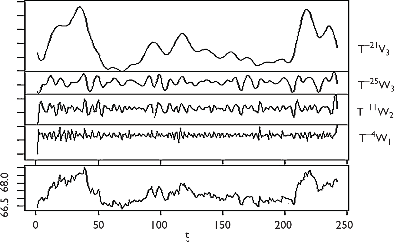
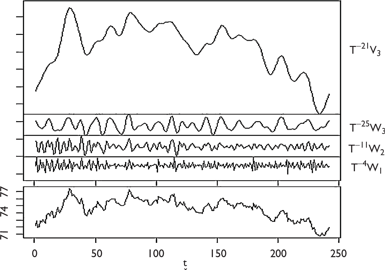
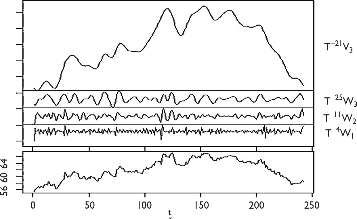
We initially investigate year-wise inherent nature of movements of three exchange rates, namely Indian rupee/US dollar, Indian rupee/euro and Indian rupee/Japanese yen, during 2011–2016 through Mandelbrot’s (1972) single fractal model. Subsequently, maximal overlap discrete wavelet transformation (MODWT) has been applied to decompose the time series of the individual exchange rates. Random forest (RF) and bagging are applied on the decomposed components for predictive modelling.

Plan of the remainder of the paper is as follows. The second section highlights the key research objectives in detail. Survey of related research has been presented in the third section. The fourth section elucidates the utilized research methodologies. Key descriptive statistics are computed to characterize the nature of exchange rates and summarized in the fifth section. The sixth section discusses the overall results and key inferences drawn. Finally, the paper is concluded in the seventh section.

Objective

Advances in computing techniques have led to greater understanding of patterns in time series data and both fractal and wavelet analyses have thrown significant light on the nature of movement of data over time. While fractal analysis enables us to determine whether the data shows strong persistent or anti-persistent characteristics, wavelet analysis enables us to break down the data into various components such as trend, random and periodic movements. In order to forecast from past time series data, it is important to first understand the inherent characteristics of the data. In this paper we take a granular approach to forecasting the exchange rate. We first apply fractal framework to understand the overall pattern of the series. Then we break down the data into various components through wavelet analysis and then forecast the exchange rate by forecasting each component, and then aggregating. In this way, each component of the series is given weightage/cognizance and also improves our understanding of the pattern. It also helps us in characterizing a series to be either trend-dominated, or periodic or purely random. Forecasting on the basis of the aggregate exchange rate robs us of our understanding of the finer details of the series. We use three exchange rates, namely the Indian rupee/US dollar rate, the Indian rupee/euro rate and the Indian rupee/Japanese yen rate to demonstrate our framework of analysis and determine its efficacy.

Related Work

Zhang and Berardi (2001) applied artificial neural networks (ANN) for forecasting the British pound/US dollar exchange rate in a univariate framework deploying lagged values of target as predictors.

Bellgard and Goldschmidt (1998) examined foreign exchange rate forecasting in terms of the random walk hypothesis (RWH). The various techniques used were random walks, exponential smoothing, auto-regressive integrated moving average (ARIMA) and ANN. The focus was on RWH and the data that was used was Australian–US dollar data. Their work was based on Bellgard (1998) where the basic objective was to explore whether ANN are superior to simple linear modelling techniques in forecasting foreign exchange rates, for different frequency data.

Shmilovici, Kahiri, Ben-Gal and Hauser (2009) used a universal variable-order Markov (VOM) model to test weak form of the efficient market hypothesis (EMH) with 12 pairs of international intra-day currency exchange rates for one year series of 1, 5, 10, 15, 20, 25 and 30 minutes. They found statistically significant compression and observed that although high-frequency series are predictable above random, the model could not generate a profitable trading strategy. They concluded that the forex market is efficient, at least most of the time.

Yu, Wang and Lai (2005) used adaptive smoothing neural networks in forecasting the exchange rate. In this model, adaptive smoothing techniques were used to adjust the neural network learning parameters automatically by tracking signals under dynamic varying environments. To verify the effectiveness of the proposed model, they used the British pound, euro and Japanese yen as the forecasting targets. Their results indicate that the model is an effective approach for foreign exchange rate forecasting.

Zhang (1994) applied ANN to search for non-linear relations in high-frequency foreign exchange time series. Three years’ (1985–1987) tick-by-tick bid prices for the Swiss franc to the US dollar exchange rate were used in this study as training data to specify predictive models for intra-day trading. The model was then tested on the same exchange rate time series in the following year (1988). In contrast to a linear model, the non-linear model used produced profit and thus prediction was relatively efficient.

Wong, Ip, Xe and Lui (2003) applied wavelets to model the movement of the US dollar against Deutsche Mark (DM) exchange rate data, and 10 steps ahead (two weeks) forecasting was compared with several other methods. In the paper, the time series was decomposed into sum of three separate components, namely trend, harmonic and irregular components. They found that under the average percentage of forecasting error (APE) criterion, the wavelet approach is the best one.

Septiarini, Abadi and Taufik (2016) considered application of wavelet fuzzy model to forecast the exchange rate between Indonesian IDR and US dollar. The wavelet fuzzy model is the combination of fuzzy Mamdani model and discrete wavelet transforms (DWT). In this paper, the data of exchange rate used was weekly exchange rate data from 1 January 2012 until 9 November 2014. The result of forecasting gave a level of accuracy of mean absolute percentage error (MAPE) of 3.45 per cent for training data and 1.74 per cent for testing the data.

Tao (2006) uses a hybrid model which integrates the wavelet neural network with genetic algorithm for predicting the exchange rate. Their model shows that the proposed model can predict exchange rate with the scale of one day, one week and other intervals. Some other papers in this area are Lebaron (1999), Baetaens, Van Den Berg and Vaudrey (1996) and Kaashoek and Van Dijk (2002).

Research Methodology

In this paper, to understand the dynamic pattern of exchange rate movements over time, initially rescaled range (R/S) analysis-based Hurst exponent (H) and fractal dimensional index (FDI) are calculated. Once the inherent patterns are identified, MODWT is applied to transform the respective exchange rate series into sub-series. Then machine learning algorithms are applied on each sub-series, and final forecast is made by aggregating the forecasted values obtained from each sub-series. For prediction, RF, an advanced ensemble machine learning tool, is employed. A brief overview of the techniques applied in this study is elucidated here.

Rescaled range (R/S) analysis: Mandelbrot and Wallis (1968) introduced R/S analysis on the basis of Hurst’s (1951) work to classify time series into pure random or biased random series. Using R/S analysis, two measures, Hurst exponent (H) and FDI, are computed to detect the presence of long-range (memory) dependence and short-range (memory) dependence in a given time series. The key steps of R/S analysis are as follows:

Step 1: The time series (R_N) of length N is initially divided into g groups of continuous sub-series of length n.

Step 2: The mean (E_g) of each sub-series Rj,g (j = 1, 2, …., n) is computed.

Step 3: The cumulative deviation of individual elements from the mean of respective sub-series is computed as

X_{j, g} = \sum_{i = 1}^{j} (R_{i, g} - E_{g}) .

(1)

Step 4: The range is calculated by the following equation:

R_{g} = m a x (X_{j, g}) - m i n (X_{j, g}) .

(2)

Step 5: The standard deviation (S_g) of individual sub-series is calculated from

S_{g} = \sqrt{(1 / n) \sum_{j = 1}^{n} {(R_{j, g} - E_{g})}^{2}} .

(3)

Step 6: Finally, the mean value of the rescaled range for all sub-series is computed as

(R / S_{n}) = (1 / A) \sum_{g = 1}^{G} (R_{d} / S_{d}) .

(4)

The Hurst exponent: The R/S statistic and Hurst coefficient (H) are asymptotically related as

(R / S_{n}) = C \times n^{H},

(5)

where C is a constant. The value of Hurst exponent (H) is generally determined through ordinary least squares (OLS) regression over a sample of increasing time horizons on the following equation:

\log {(R / S)}_{n} = \log C + H \log_{n}

(6)

The Hurst exponent (H) can take any value in the range [0, 1]. Theoretically, an estimated H value of 0.5 means that the series is ideally following an independent and identically distributed (iid) Gaussian random walk model. On the other hand, if the value of H is different from 0.5, then the series is said to exhibit characteristics of fractional Brownian motion or biased random walk. Persistent or long memory nature of a time series is established when the value of H is greater than 0.5. If the computed value of H is less than 0.5, then the series is said to be governed by anti-persistent pattern.

Fractal dimensional index (FDI): FDI is a quantifiable measurement index that helps understand the dynamics of any chaotic system. Fractals can be thought of as objects with self-similar constituents. Any financial time series can be thought of as a series of fractals that appear similar across a range of time periods. Through determination of FDI, dynamics of stock markets can be measured for predictability, complexity and irregularity. The FDI (D) and Hurst exponent (H) are related by the following equation:

D = 2 - H .

(7)

Since the range of H is 0 to 1, the values of D varies in the range of 1 to 2. For a given sequence, a D value of 1.5 signifies that the sequence follows random walk. Persistent and anti-persistent behaviour of a sequence correspond to $1 < D < 1.5$ and $1.5 < D < 2$ respectively. For time series data on financial markets, an FDI value closer to 1 infers trending market in one direction, that is, presence of long-range dependence. High volatile periods are followed by high volatile periods and low volatile periods by low volatile periods. This long-range dependence is also termed as ‘Joseph’s Effect’, and is drawn from the Old Testament prophecy of seven years of plenty followed by seven years of famine. Alternatively, when FDI value is closer to 2, an exact opposite situation prevails, that is, high volatility is followed by low volatility and low volatility by high volatility. This short-range dependence is termed as ‘Noah’s Effect’.

Maximal overlap discrete wavelet transform (MODWT): The objective of wavelet analysis is to decompose a signal into time scale space. It is a filtering operation that segregates a time series into coefficients related to variation over a set of scales. It can effectively separate non-linearity and presence of other erratic features in financial time series without affecting inherent features such as spillovers, clustering and heteroscedasticity. Ramsey and Zhang (1997) applied wavelet decomposition to examine foreign exchange rate dynamics. Gencay, Selçuk and Whitcher (2001) showed the effectiveness of wavelet filtering to deal with non-stationary and time-varying features of time series. Khandelwal, Adhikari and Verma (2015) applied ARIMA and ANN models on decomposed time series data using discrete wavelength transformation (DWT) for efficient forecasting. Ghosh and Chaudhuri (2016) decomposed time series data on Chicago Board of Options Exchange Implied Volatility Index (CBOE VIX), National Stock Exchange Implied Volatility Index (India VIX) and Historic Volatility (HV) via DWT using Haar wavelets and applied RF and ARIMA for forecasting.

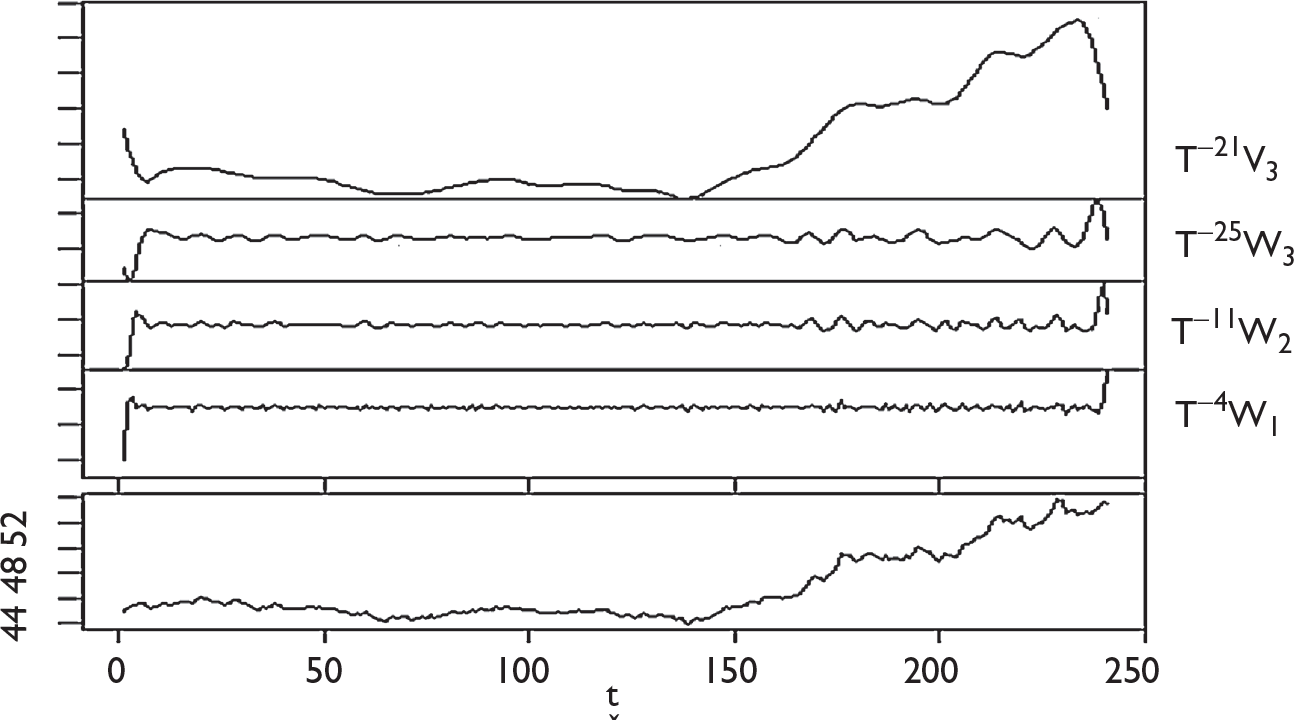
In the wavelet analysis, the original function $(f (t))$ is translated and dilated onto father $(φ (t))$ and mother $(ψ (t))$ wavelets at different scales. The mother $(ψ (t))$ wavelets represent the details having unit energy and 0 mean, whereas the father $(φ (t))$ wavelets define the approximations with mean value of 1. Mathematically, it can be expressed as

\int φ (t) d t = 1

(8)

\int^{​} ψ (t) d t = 0.

(9)

If r_it denotes the value of time series i at time t, then the time series is approximated using the detail coefficients $ψ_{j, k}^{r_{i}}$ and approximation coefficients $φ_{J, k}^{r_{i}}$ as given by equation (3):

r_{i t} = s_{J}^{r_{i}} (t) + d_{J}^{r_{i}} (t) + d_{J - 1}^{r_{i}} (t) + \dots + d_{1}^{r_{i}} (t),

(10)

where

s_{J}^{r_{i}} (t) = \sum_{k} φ_{J, k}^{r_{i}} ϕ_{J, k} (t)

(11)

d_{j}^{r_{i}} (t) = \sum_{k} ψ_{J, k}^{r_{i}} ω_{j, k} (t)

(12)

ϕ_{J, k} (t) = 2^{- J / 2} ϕ (\frac{t - 2^{J} k}{2^{J}})

(13)

ω_{j, k} (t) = 2^{- j / 2} ω (\frac{t - 2^{j} k}{2^{j}}) .

(14)

For j = 1, 2, …, J.

As discussed, $s_{J}^{r_{i}} (t)$ and $d_{j}^{r_{i}} (t)$ are known as approximation (low frequency) and detail levels (high frequency) respectively. The discrete wavelet transform of any function f (t) is expressed as

\tilde{W_{l, k}} = \int_{- \infty}^{\infty} f (t) ψ_{l, k} (t) d t

(15)

The inverse wavelet transform is defined as

f (t) = \sum_{l = - \infty}^{\infty} \sum_{k = - \infty}^{\infty} \tilde{W_{l, k}} \times ψ_{l, k} (t)

(16)

In general, traditional DWT method operates on the principle of convolution for decomposition. There are several advantages of MODWT over DWT for decomposition of time series. First of all, unlike DWT, MODWT does not require the dataset to be dyadic. It is also invariant to circular shift. Overall, MODWT is a robust and non-orthogonal transformation that keeps the down-sampled values at each level of decomposition.

Random forest (RF): RF proposed by Breiman (2001) is an ensemble approach for prediction where each of the classifiers is a decision tree. It is a general-purpose machine learning tool composed of decision trees as base learners. Decision trees are constructed in randomly selected sub-spaces data. Each tree in the ensembles is randomly selected. At each node of that selected tree, the best variables to split are chosen from the training set. RF can also be built using bootstrap aggregation (bagging) for ensemble learning (Breiman, 1996). Such form of RF is termed as Forest-RI. The assignment of class label of an unknown instance (for classification) or prediction of continuous outcome (regression) is performed using majority voting or averaging strategy. RF, robust to outliers, can handle very large number of input attributes. It avoids over-fitting problem when the number of trees in forest is large due to convergence of generalization error. It has extensively been used carrying out predictive modelling to study complex systems in presence of non-linearity as reported in literature (Liu, Wang, Wang, & Li, 2013; Xie, Li, Ngai, & Ying, 2009, etc.).

Bagging: Similar to RF, bagging (bootstrap aggregating) is also an ensemble-based approach where prediction is made based on several decision trees constructed using bootstrapped samples (Simidjievski, Todorovski, & Dzeroski, 2015). For each bootstrap sample drawn from training dataset, a regression tree is built. The final model is average of all the individual regression trees.

The major difference between RF and bagging is that unlike RF, in bagging, decision trees are built considering all the features. They are not chosen randomly. For regression tasks, bagging reduces the variance of unstable learning methods leading to improved prediction. In general, the steps involved in learning process of bagging are as follows:

Step 1: Bootstrapped samples are drawn from the training data.

Step 2: For each sample, a decision tree is grown, and at each node of the tree

Step 2.1: Select the best feature from the set of all available features.

Step 2.2: Find the best split.

Step 2.3: Repeat Steps 2.1 and 2.2 until the tree is fully grown.

Step 3: Combine the outcome of individual trees to get the final outcome.

Like RF, bagging too has successfully been applied in discovering and comprehending complex patterns (Lemmens & Croux, 2006; Zheng, Caixin, Jian, Qing, & Weigen, 2011).

Analysis on Data

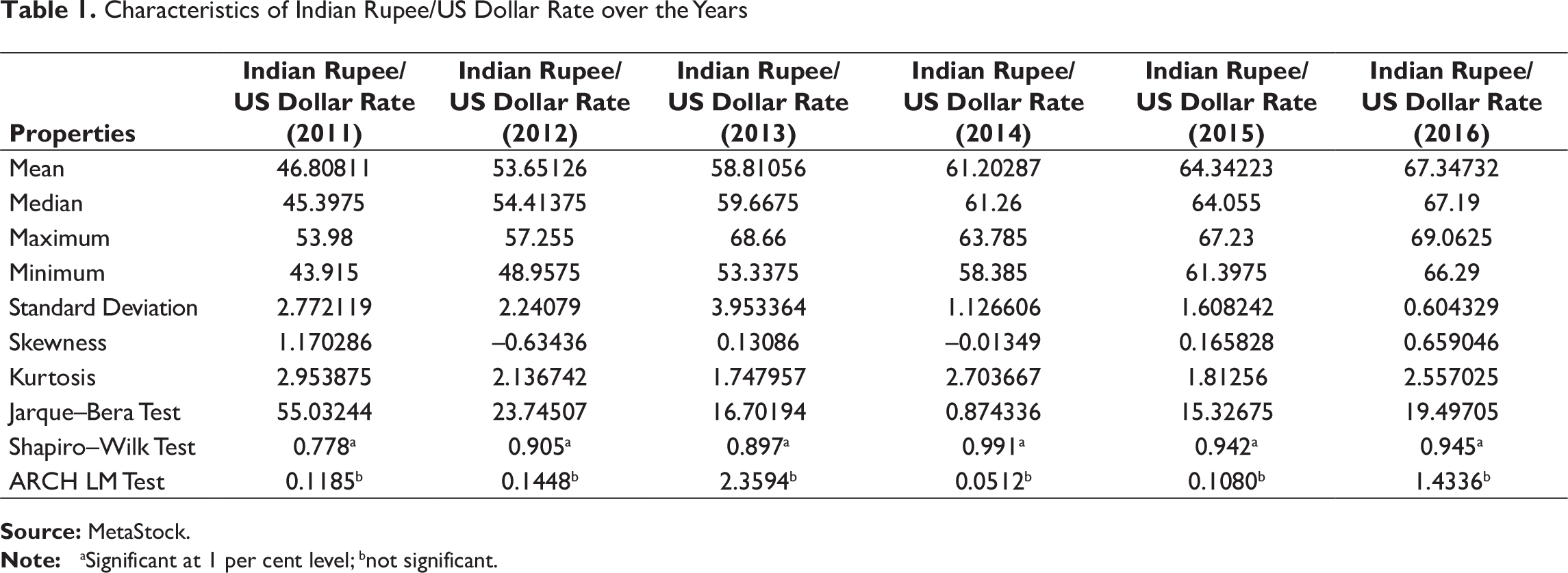
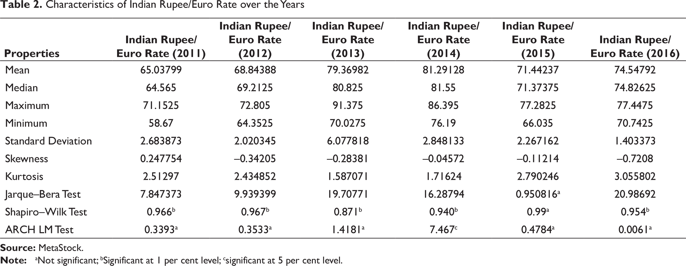
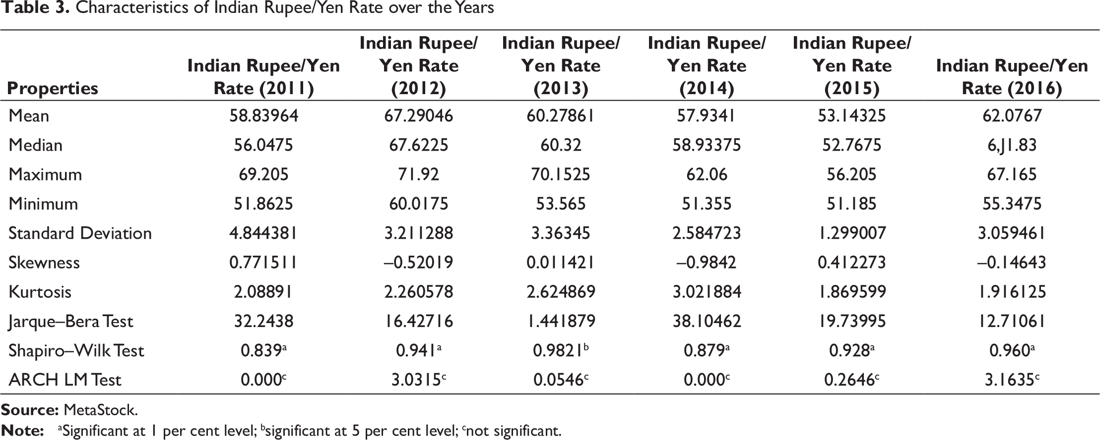
Data on exchange rates of Indian rupee/US dollar, Indian rupee/euro and Indian rupee/yen for the years 2011–2016 have been compiled from MetaStock, and the descriptive statistics are presented in Tables 1–3.

It is evident from both Jarque–Bera and Shapiro–Wilk tests that Indian rupee/US dollar rate did not follow normal distribution over the years. Auto-regressive conditional heteroscedasticity (ARCH) Lagrange multiplier (LM) test confirms that year wise, there was no effect of conditional heteroscedasticity in movements of Indian rupee/US dollar exchange rate.

Like Indian rupee/US dollar rate, normality assumption is rejected for year-wise Indian rupee/euro rates. No significant effects of conditional heteroscedasticity have been observed, except for year 2014.

For the Indian rupee/yen rate, Jarque–Bera and Shapiro–Wilk tests statistics show that Indian rupee/yen rates do not follow normal distribution. ARCH LM test reveals presence of conditional heteroscedasticity in year-wise movement.

Results and Analysis

Fractal inspection of exchange rates: At first, values of Hurst exponent (H) and FDI are estimated to characterize year-wise dynamics of movement of Indian rupee/US dollar rate, the Indian rupee/euro rate and the Indian rupee/Japanese yen rate over the time periods considered in the study and to test the Brownian motion hypothesis. Correlation between periods (CN), an index to quantify the impact of persistent or anti-persistence pattern if prevails, has also been calculated according to

Table 1.

Characteristics of Indian Rupee/US Dollar Rate over the Years

Properties	Indian Rupee/US Dollar Rate (2011)	Indian Rupee/US Dollar Rate (2012)	Indian Rupee/US Dollar Rate (2013)	Indian Rupee/US Dollar Rate (2014)	Indian Rupee/US Dollar Rate (2015)	Indian Rupee/US Dollar Rate (2016)
Mean	46.80811	53.65126	58.81056	61.20287	64.34223	67.34732
Median	45.3975	54.41375	59.6675	61.26	64.055	67.19
Maximum	53.98	57.255	68.66	63.785	67.23	69.0625
Minimum	43.915	48.9575	53.3375	58.385	61.3975	66.29
Standard Deviation	2.772119	2.24079	3.953364	1.126606	1.608242	0.604329
Skewness	1.170286	–0.63436	0.13086	–0.01349	0.165828	0.659046
Kurtosis	2.953875	2.136742	1.747957	2.703667	1.81256	2.557025
Jarque–Bera Test	55.03244	23.74507	16.70194	0.874336	15.32675	19.49705
Shapiro–Wilk Test	0.778^a	0.905^a	0.897^a	0.991^a	0.942^a	0.945^a
ARCH LM Test	0.1185^b	0.1448^b	2.3594^b	0.0512^b	0.1080^b	1.4336^b

Source: MetaStock.

Note: ^aSignificant at 1 per cent level; ^bnot significant.

Table 2.

Characteristics of Indian Rupee/Euro Rate over the Years

Properties	Indian Rupee/Euro Rate (2011)	Indian Rupee/Euro Rate (2012)	Indian Rupee/Euro Rate (2013)	Indian Rupee/Euro Rate (2014)	Indian Rupee/Euro Rate (2015)	Indian Rupee/Euro Rate (2016)
Mean	65.03799	68.84388	79.36982	81.29128	71.44237	74.54792
Median	64.565	69.2125	80.825	81.55	71.37375	74.82625
Maximum	71.1525	72.805	91.375	86.395	77.2825	77.4475
Minimum	58.67	64.3525	70.0275	76.19	66.035	70.7425
Standard Deviation	2.683873	2.020345	6.077818	2.848133	2.267162	1.403373
Skewness	0.247754	–0.34205	–0.28381	–0.04572	–0.11214	–0.7208
Kurtosis	2.51297	2.434852	1.587071	1.71624	2.790246	3.055802
Jarque–Bera Test	7.847373	9.939399	19.70771	16.28794	0.950816^a	20.98692
Shapiro–Wilk Test	0.966^b	0.967^b	0.871^b	0.940^b	0.99^a	0.954^b
ARCH LM Test	0.3393^a	0.3533^a	1.4181^a	7.467^c	0.4784^a	0.0061^a

Source: MetaStock.

Note: ^aNot significant; ^bSignificant at 1 per cent level; ^csignificant at 5 per cent level.

Table 3.

Characteristics of Indian Rupee/Yen Rate over the Years

Properties	Indian Rupee/Yen Rate (2011)	Indian Rupee/Yen Rate (2012)	Indian Rupee/Yen Rate (2013)	Indian Rupee/Yen Rate (2014)	Indian Rupee/Yen Rate (2015)	Indian Rupee/Yen Rate (2016)
Mean	58.83964	67.29046	60.27861	57.9341	53.14325	62.0767
Median	56.0475	67.6225	60.32	58.93375	52.7675	6,J1.83
Maximum	69.205	71.92	70.1525	62.06	56.205	67.165
Minimum	51.8625	60.0175	53.565	51.355	51.185	55.3475
Standard Deviation	4.844381	3.211288	3.36345	2.584723	1.299007	3.059461
Skewness	0.771511	–0.52019	0.011421	–0.9842	0.412273	–0.14643
Kurtosis	2.08891	2.260578	2.624869	3.021884	1.869599	1.916125
Jarque–Bera Test	32.2438	16.42716	1.441879	38.10462	19.73995	12.71061
Shapiro–Wilk Test	0.839^a	0.941^a	0.9821^b	0.879^a	0.928^a	0.960^a
ARCH LM Test	0.000^c	3.0315^c	0.0546^c	0.000^c	0.2646^c	3.1635^c

Source:MetaStock.

Note: ^aSignificant at 1 per cent level; ^bsignificant at 5 per cent level; ^cnot significant

C_{N} = 2^{(2 H - 1)} - 1

(17)

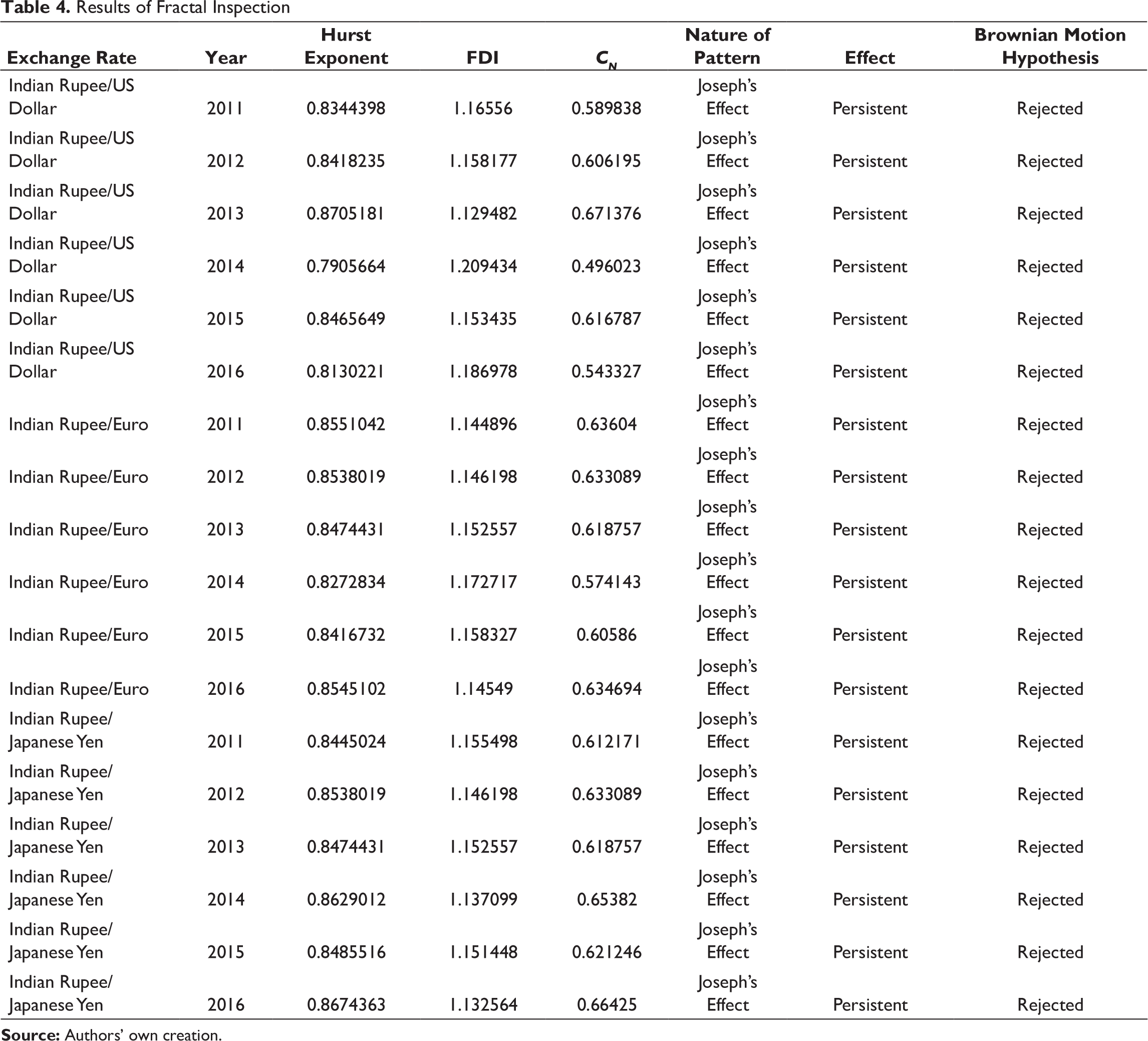
If a time series is found to be perfectly random (H = 0), value of C_N is 0. For a persistent time series, C_N is positive. An anti-persistent time series results in negative correlation. A C_N value of 0.2 implies that 20 per cent of the entire data is influenced by past. Tables 4 and 5 narrate the results of fractal investigation of the respective exchange rates over the years.

Results, manifested through values of Hurst exponent and FDI clearly indicate that the yearly movements of three exchange rates exhibit strong presence of persistent pattern. Correlation between periods indicate that on an average, 60 per cent of the data on exchange rates are influenced by historical values. Presence of fractal structure and significant values of correlation between periods justifies the dominance of trend components in exchange rate dynamics and provides support for univariate predictive modelling framework based on lagged values for forecasting purpose.

MODWT analysis: We have considered ‘Haar’ wavelets for three levels of decomposition for individual year-wise exchange rates. Hence, three wavelet coefficients and one scaling coefficient will be obtained in the said decomposition process. Figures 1– 6 graphically illustrate the MODWT decomposition of some of the selected series.

Figure 1.

Source: ‘Wavelets’ package of R.

Table 4.

Results of Fractal Inspection

Exchange Rate	Year	Hurst Exponent	FDI	C _N	Nature of Pattern	Effect	Brownian Motion Hypothesis
Indian Rupee/US Dollar	2011	0.8344398	1.16556	0.589838	Joseph’s Effect	Persistent	Rejected
Indian Rupee/US Dollar	2012	0.8418235	1.158177	0.606195	Joseph’s Effect	Persistent	Rejected
Indian Rupee/US Dollar	2013	0.8705181	1.129482	0.671376	Joseph’s Effect	Persistent	Rejected
Indian Rupee/US Dollar	2014	0.7905664	1.209434	0.496023	Joseph’s Effect	Persistent	Rejected
Indian Rupee/US Dollar	2015	0.8465649	1.153435	0.616787	Joseph’s Effect	Persistent	Rejected
Indian Rupee/US Dollar	2016	0.8130221	1.186978	0.543327	Joseph’s Effect	Persistent	Rejected
Indian Rupee/Euro	2011	0.8551042	1.144896	0.63604	Joseph’s Effect	Persistent	Rejected
Indian Rupee/Euro	2012	0.8538019	1.146198	0.633089	Joseph’s Effect	Persistent	Rejected
Indian Rupee/Euro	2013	0.8474431	1.152557	0.618757	Joseph’s Effect	Persistent	Rejected
Indian Rupee/Euro	2014	0.8272834	1.172717	0.574143	Joseph’s Effect	Persistent	Rejected
Indian Rupee/Euro	2015	0.8416732	1.158327	0.60586	Joseph’s Effect	Persistent	Rejected
Indian Rupee/Euro	2016	0.8545102	1.14549	0.634694	Joseph’s Effect	Persistent	Rejected
Indian Rupee/Japanese Yen	2011	0.8445024	1.155498	0.612171	Joseph’s Effect	Persistent	Rejected
Indian Rupee/Japanese Yen	2012	0.8538019	1.146198	0.633089	Joseph’s Effect	Persistent	Rejected
Indian Rupee/Japanese Yen	2013	0.8474431	1.152557	0.618757	Joseph’s Effect	Persistent	Rejected
Indian Rupee/Japanese Yen	2014	0.8629012	1.137099	0.65382	Joseph’s Effect	Persistent	Rejected
Indian Rupee/Japanese Yen	2015	0.8485516	1.151448	0.621246	Joseph’s Effect	Persistent	Rejected
Indian Rupee/Japanese Yen	2016	0.8674363	1.132564	0.66425	Joseph’s Effect	Persistent	Rejected

Source:Authors’ own creation.

Table 5.

Descriptive Statistics of Hurst Exponent, FDI and C_N

Measure	Minimum	Maximum	Average	Median	Standard Deviation	Skewness	Kurtosis
Hurst Exponent	0.7906	0.8629	0.8399	0.8470	0.0203	–1.2123	0.3776
FDI	1.1371	1.2094	1.1601	1.1530	0.0203	1.2123	0.3776
C_N	0.4960	0.6538	0.6025	0.6178	0.0442	–1.1728	0.2846

Source:Authors’ own creation.

Figure 2.

Source: ‘Wavelets’ package of R.

Figure 3.

Source: ‘Wavelets’ package of R.

Figure 4.

Source: ‘Wavelets’ package of R.

Figure 5.

Source: ‘Wavelets’ package of R.

Figure 6.

Source: ‘Wavelets’ package of R.

Predictive modelling: As stated earlier, RF has been applied on each decomposed sub-series obtained through MODWT to get the forecasted values. Final forecast values are arrived at by taking the sum over forecasts obtained in all sub-series of respective series. So, the final forecast of Indian rupee/US dollar rate of a given year is determined as follows:

(Indian rupee/US dollar)_{Final_Forecast} = (Indian rupee/US dollar_V3)_{RF_Forecast} + (Indian rupee/US dollar_W1)_{RF_Forecast} + (Indian rupee/US dollar_W2)_{RF_Forecast} + (Indian rupee/US dollar_W3)_{RF_Forecast,}

where (Indian rupee/US dollar_V3)_{RF_Forecast} is the forecast by RF on scaling component and (Indian rupee/US dollar_W1)_{RF_Forecast}, (Indian rupee/US dollar_W1)_{RF_Forecast} and (Indian rupee/US dollar_W1)_{RF_Forecast} are the forecasts generated by RF for respective wavelet components. In a similar manner, final prediction is made for Indian rupee/euro and Indian Rupee/yen rates.

In this paper, univariate predictive modelling is adopted considering one-day-lagged, two-days-lagged, three-days-lagged and four-days-lagged values as independent variables. RF has simply been used to map the functional relationships as given in the following equation.

E (t) = f (E (t - 1), E (t - 2), E (t - 3), E (t - 4)),

where E(t) is the exchange rate at day t and

E (t - 1), E (t - 2), E (t - 3), E (t - 4)

represent the values of exchange rate at (t - 1), (t - 2), (t - 3) days respectively.

To implement the algorithms, ‘caTools’ (to generate training and test datasets), ‘randomForest’ (to simulate RF) and ‘ipred’ (to run bagging) packages of R have been used. The codes for implementing the respective predictive models are as follows:

Data<-read.csv (file.choose()) \\ To load dataset (year-wise exchange rate) in R require (caTools) \\ To load the package

set.seed (101) \\ For reuse purpose

sample = sample.split (Data$Target, SplitRatio = 0.85) \\ For splitting dataset

train = subset (Data, sample = TRUE) \\ Generating training data

test = subset (Data, sample = FALSE) \\ Generating test data

require (randomForest) \\ To load the requisite package for RF

fmodel_RF<-randomForest (train$Target~., data = train, ntree = 200, importance = T) \\ For building RF model with 200 trees

U<-predict (fmodel_RF, test) \\ To predict on test dataset with built RF model

Require (ipred) \\ To load the requisite package for bagging

fmodel_Bagging<-bagging (train$Target~., data = train, nbagg = 200) \\ For building bagging model with 200 base learners

U<-predict (fmodel_Bagging, test) \\ To predict on test dataset with constructed bagging model

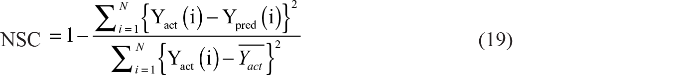
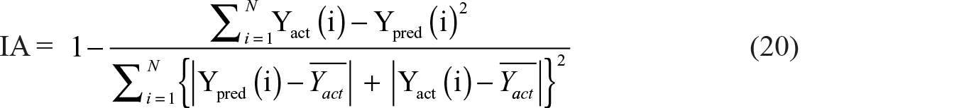
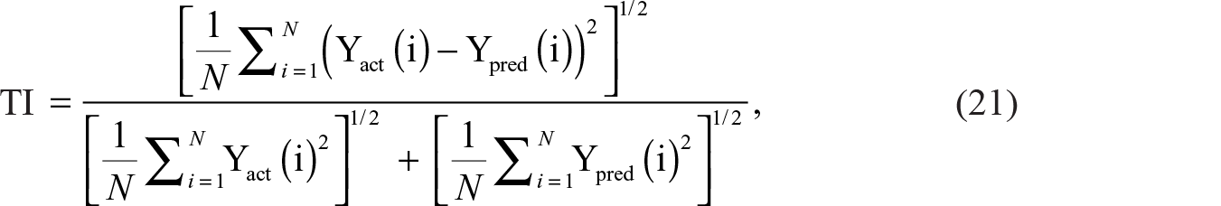
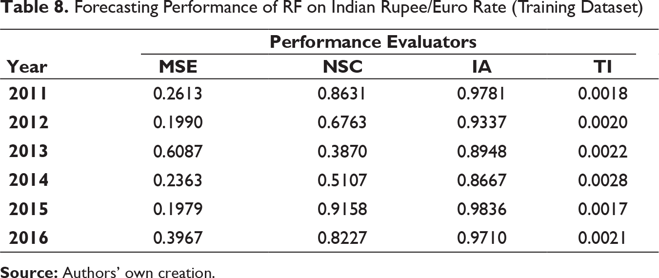
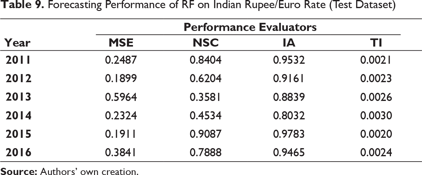
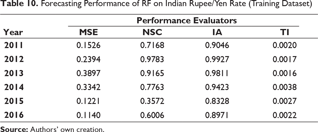
To evaluate the performance of predictive modelling, four quantitative measures, namely mean squared error (MSE), Nash–Sutcliffe coefficients (NSC), index of agreement (IA) and Theil inequality (TI) are computed. These measures are defined as follows:

MSE = \frac{1}{N} \sum_{i = 1}^{N} {Y_{act} (i) - Y_{pred} (i)}^{2} \frac{1}{N} \sum_{i = 1}^{N} {Y_{act} (i) - Y_{pred} (i)}^{2}

(18)

NSC = 1 - \frac{\sum_{i = 1}^{N} {Y_{act} (i) - Y_{pred} (i)}^{2}}{\sum_{i = 1}^{N} {Y_{act} (i) - \bar{Y_{a c t}}}^{2}}

(19)

IA - \frac{\sum_{i = 1}^{N} Y_{act} (i) - Y_{pred} {(i)}^{2}}{\sum_{i = 1}^{N} {| Y_{pred} (i) - \bar{Y_{a c t}} | + | Y_{act} (i) - \bar{Y_{a c t}} |}^{2}}

(20)

TI = \frac{{[\frac{1}{N} \sum_{i = 1}^{N} {(Y_{act} (i) - Y_{pred} (i))}^{2}]}^{1 / 2}}{{[\frac{1}{N} \sum_{i = 1}^{N} Y_{act} {(i)}^{2}]}^{1 / 2} + {[\frac{1}{N} \sum_{i = 1}^{N} Y_{pred} {(i)}^{2}]}^{1 / 2}},

(21)

where Y_act(i) and Y_pred(i) are actual and predicted outcomes. Values of MSE must be as low as possible to indicate efficient prediction; ideally, a value of 0 signifies no error. NSC can range between –∞ to 1. NSC value of 1 corresponds to a perfect match between model and observations, whereas value of less than 0 occurs when the observed mean is a better predictor than the modeller. Essentially, closer the value of NSE to 1, better is the predictive performance. The range of IA lies between 0 (no fit) and 1 (perfect fit). TI values range between 0 and 1. They should be close to 0 for good prediction, while a value close to 1 implies no prediction at all.

Results of RF-based predictive analysis: To perform predictive modelling, initially the dataset of individual exchange rates of respective year has been partitioned into training/calibration (85%) and test (15%) data. As the performance of the RF algorithm is highly dependent on number of decision trees, it has been varied in the range of 100 to 1,000 with an interval of 100. Number of variables for branching operations in constituent decision trees have been fixed as three. Hence, total 10 experimental trials have been carried out. Average scores of MSE, NSC, IA and TI of 10 experimental trials are computed to evaluate the forecasting performance of RF as shown in the Tables 6–17.

Table 6.

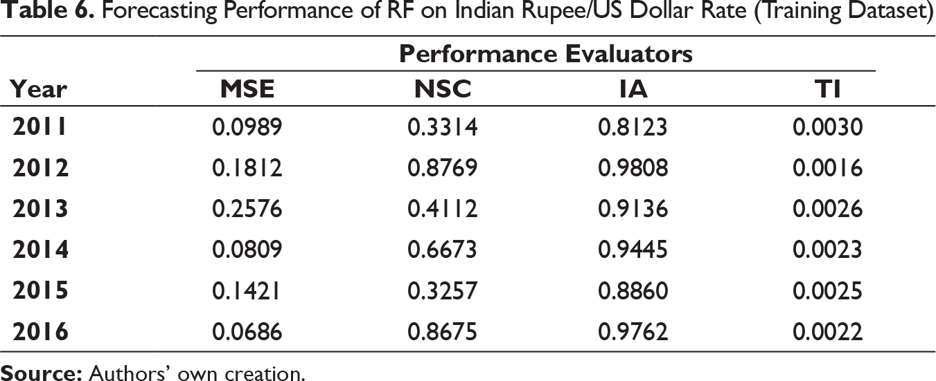
Forecasting Performance of RF on Indian Rupee/US Dollar Rate (Training Dataset)

Year	Performance Evaluators
Year	MSE	NSC	IA	TI
2011	0.0989	0.3314	0.8123	0.0030
2012	0.1812	0.8769	0.9808	0.0016
2013	0.2576	0.4112	0.9136	0.0026
2014	0.0809	0.6673	0.9445	0.0023
2015	0.1421	0.3257	0.8860	0.0025
2016	0.0686	0.8675	0.9762	0.0022

Source: Authors’ own creation.

Table 7.

Forecasting Performance of RF on Indian Rupee/US Dollar Rate (Test Dataset)

Year	Performance Evaluators
Year	MSE	NSC	IA	TI
2011	0.0924	0.2830	0.7478	0.0033
2012	0.1680	0.8505	0.9675	0.0019
2013	0.2333	0.3300	0.8733	0.0027
2014	0.0654	0.6171	0.8767	0.0025
2015	0.1037	0.2829	0.8595	0.0028
2016	0.0613	0.7911	0.9450	0.0025

Source:Authors’ own creation.

Table 8.

Forecasting Performance of RF on Indian Rupee/Euro Rate (Training Dataset)

Year	Performance Evaluators
Year	MSE	NSC	IA	TI
2011	0.2613	0.8631	0.9781	0.0018
2012	0.1990	0.6763	0.9337	0.0020
2013	0.6087	0.3870	0.8948	0.0022
2014	0.2363	0.5107	0.8667	0.0028
2015	0.1979	0.9158	0.9836	0.0017
2016	0.3967	0.8227	0.9710	0.0021

Source:Authors’ own creation.

Table 9.

Forecasting Performance of RF on Indian Rupee/Euro Rate (Test Dataset)

Year	Performance Evaluators
Year	MSE	NSC	IA	TI
2011	0.2487	0.8404	0.9532	0.0021
2012	0.1899	0.6204	0.9161	0.0023
2013	0.5964	0.3581	0.8839	0.0026
2014	0.2324	0.4534	0.8032	0.0030
2015	0.1911	0.9087	0.9783	0.0020
2016	0.3841	0.7888	0.9465	0.0024

Source:Authors’ own creation.

Table 10.

Forecasting Performance of RF on Indian Rupee/Yen Rate (Training Dataset)

Year	Performance Evaluators
Year	MSE	NSC	IA	TI
2011	0.1526	0.7168	0.9046	0.0020
2012	0.2394	0.9783	0.9927	0.0017
2013	0.3897	0.9165	0.9811	0.0016
2014	0.3342	0.7763	0.9423	0.0038
2015	0.1221	0.3572	0.8328	0.0027
2016	0.1140	0.6006	0.8971	0.0022

Source:Authors’ own creation.

Table 11.

Forecasting Performance of RF on Indian Rupee/Yen Rate (Test Dataset)

Year	Performance Evaluators
Year	MSE	NSC	IA	TI
2011	0.1307	0.6311	0.8734	0.0026
2012	0.2307	0.9556	0.9887	0.0024
2013	0.3786	0.8805	0.97	0.0021
2014	0.3102	0.6527	0.90	0.0046
2015	0.1091	0.2911	0.8017	0.0031
2016	0.1065	0.5267	0.8208	0.0027

Source:Authors’ own creation.

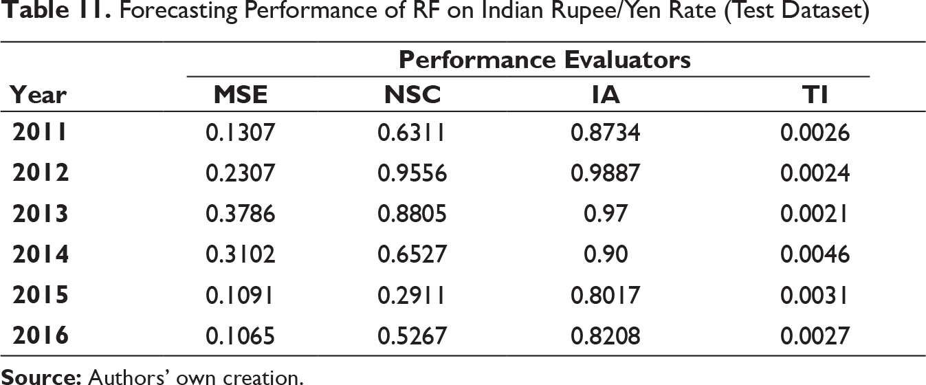
It can be clearly observed that the values of MSE and TI are substantially low for all three exchange rates on both training and test dataset for all six years. IA values are on higher side as well. On few occasions, it can be seen that the NSC values are not as high as compared to IA but not close to 0 also. It can thus be inferred that MODWT–RF-based framework can be effectively deployed for forecasting the respective exchange rates in the univariate framework used.

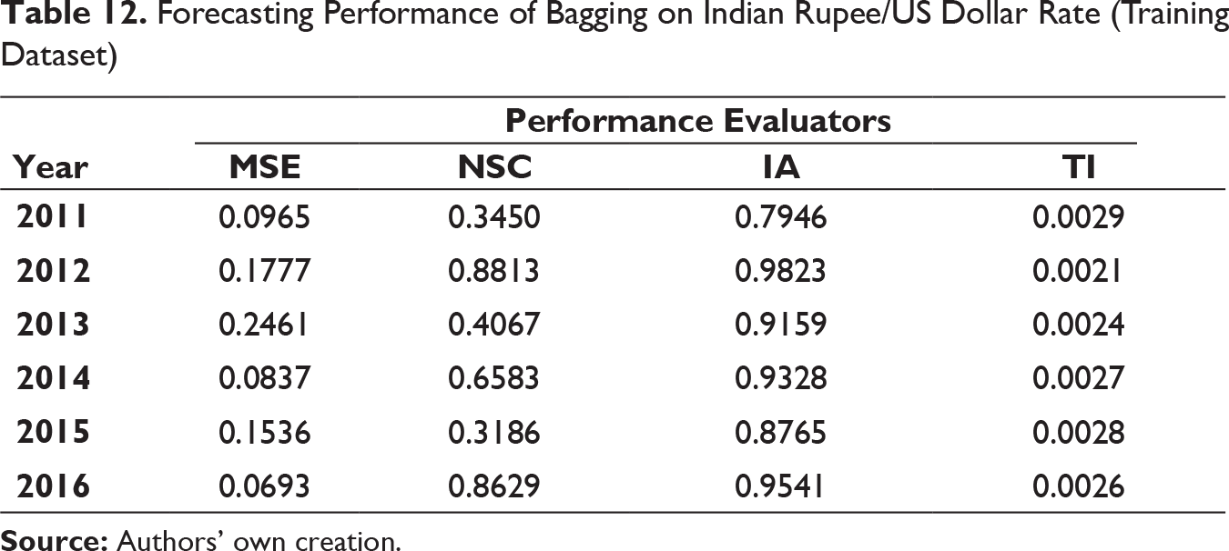
Results of bagging-based predictive analysis: Like RF, number of features for branching operations of constituent trees has been fixed as three in bagging as well. Number of decision trees are varied to perform the trials as planned. Results are summarized and discussed further.

Table 12.

Forecasting Performance of Bagging on Indian Rupee/US Dollar Rate (Training Dataset)

Year	Performance Evaluators
Year	MSE	NSC	IA	TI
2011	0.0965	0.3450	0.7946	0.0029
2012	0.1777	0.8813	0.9823	0.0021
2013	0.2461	0.4067	0.9159	0.0024
2014	0.0837	0.6583	0.9328	0.0027
2015	0.1536	0.3186	0.8765	0.0028
2016	0.0693	0.8629	0.9541	0.0026

Source:Authors’ own creation.

Table 13.

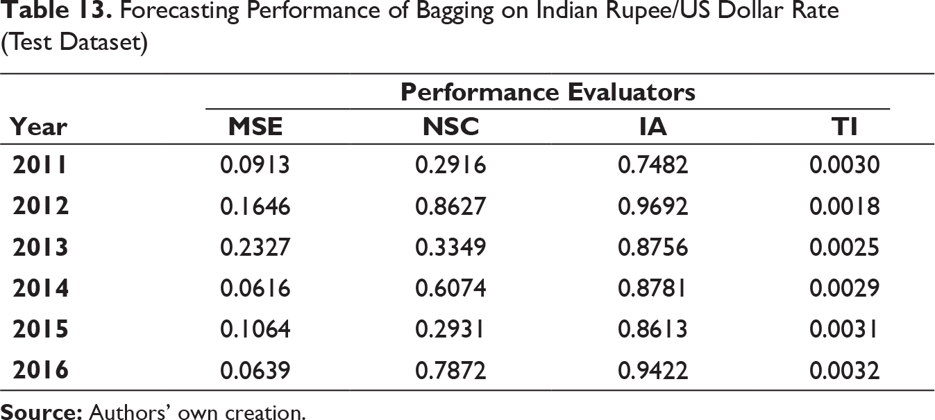
Forecasting Performance of Bagging on Indian Rupee/US Dollar Rate (Test Dataset)

Year	Performance Evaluators
Year	MSE	NSC	IA	TI
2011	0.0913	0.2916	0.7482	0.0030
2012	0.1646	0.8627	0.9692	0.0018
2013	0.2327	0.3349	0.8756	0.0025
2014	0.0616	0.6074	0.8781	0.0029
2015	0.1064	0.2931	0.8613	0.0031
2016	0.0639	0.7872	0.9422	0.0032

Source:Authors’ own creation.

Table 14.

Forecasting Performance of Bagging on Indian Rupee/Euro Rate (Training Dataset)

Year	Performance Evaluators
Year	MSE	NSC	IA	TI
2011	0.2679	0.8577	0.9659	0.0019
2012	0.2041	0.6774	0.9280	0.0023
2013	0.6059	0.3883	0.8916	0.0024
2014	0.2405	0.5136	0.8544	0.0027
2015	0.2021	0.9229	0.9815	0.0014
2016	0.3884	0.8214	0.9722	0.0017

Source:Authors’ own creation.

Table 15.

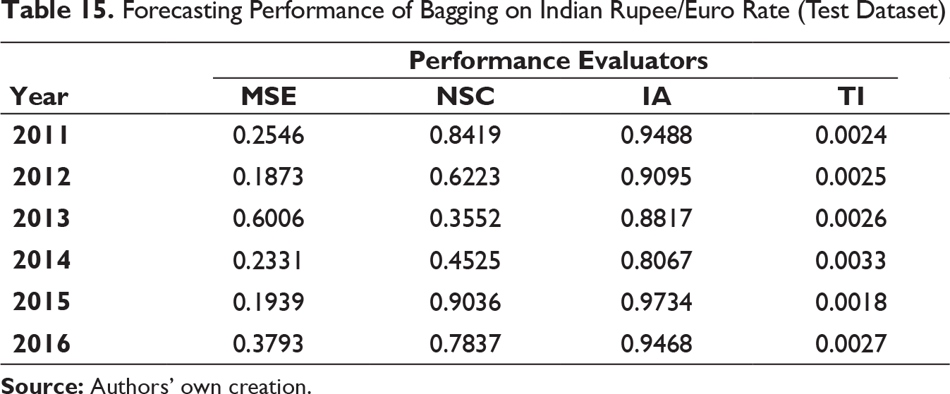
Forecasting Performance of Bagging on Indian Rupee/Euro Rate (Test Dataset)

Year	Performance Evaluators
Year	MSE	NSC	IA	TI
2011	0.2546	0.8419	0.9488	0.0024
2012	0.1873	0.6223	0.9095	0.0025
2013	0.6006	0.3552	0.8817	0.0026
2014	0.2331	0.4525	0.8067	0.0033
2015	0.1939	0.9036	0.9734	0.0018
2016	0.3793	0.7837	0.9468	0.0027

Source:Authors’ own creation.

Table 16.

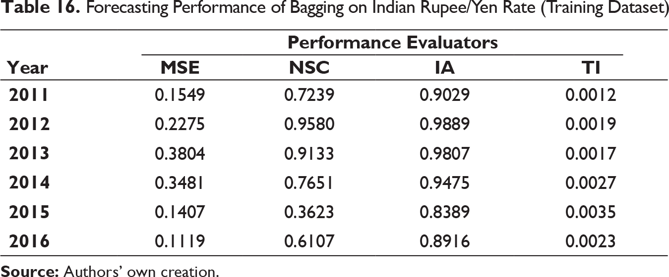
Forecasting Performance of Bagging on Indian Rupee/Yen Rate (Training Dataset)

Year	Performance Evaluators
Year	MSE	NSC	IA	TI
2011	0.1549	0.7239	0.9029	0.0012
2012	0.2275	0.9580	0.9889	0.0019
2013	0.3804	0.9133	0.9807	0.0017
2014	0.3481	0.7651	0.9475	0.0027
2015	0.1407	0.3623	0.8389	0.0035
2016	0.1119	0.6107	0.8916	0.0023

Source:Authors’ own creation.

Table 17.

Forecasting Performance of Bagging on Indian Rupee/Yen Rate (Test Dataset)

Year	Performance Evaluators
Year	MSE	NSC	IA	TI
2011	0.1254	0.6406	0.8649	0.0031
2012	0.2417	0.9527	0.9865	0.0014
2013	0.3867	0.8724	0.9681	0.0024
2014	0.3065	0.6619	0.8942	0.0049
2015	0.1142	0.2883	0.8126	0.0024
2016	0.1123	0.5259	0.8316	0.0035

Source:Authors’ own creation.

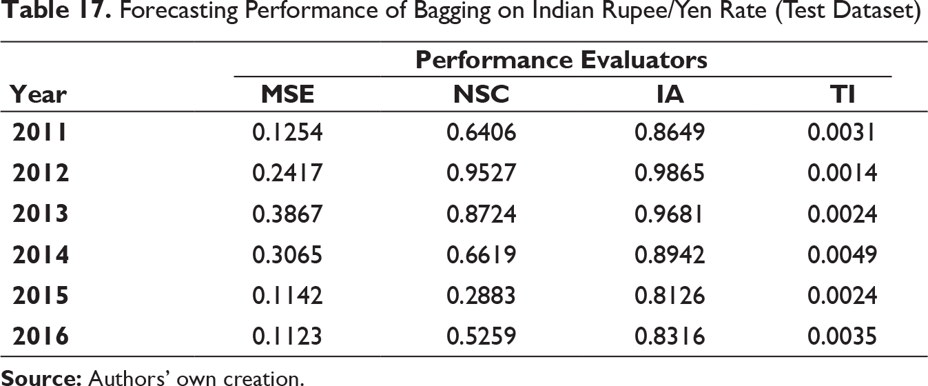
Similar to the previous model, that is, MODWT–RF, MSE and TI values have been found to be low and IA values are on higher side on all the occasions. The similar trend NSC values for MODWT–RF framework have been reflected in MODWT–bagging model too. Thus, MODWT–bagging forecasting model can also be used for effective prediction.

For fine-tuning our methodology, we have made a comparative analysis of performance of MODWT–RF and MODWT–bagging measured in terms of MSE values, using statistical t-test on sample trials of test datasets. Table 18 summarizes the results.

Table 18.

Results of Comparative Analysis

Exchange Rate	Year	Test Statistic
Indian Rupee/US Dollar	2011	1.792176a (two tailed)
	2012	12.23088b (two tailed)
	2013	1.512653a (two tailed)
	2014	12.07436b (two tailed)
	2015	–14.6956b (two tailed)
	2016	–13.72774b (two tailed)
Indian Rupee/Euro	2011	–14.873245b (two tailed)
	2012	6.421518b (two tailed)
	2013	–11.706512b (two tailed)
	2014	1.326947a (two tailed)
	2015	–13.104363b (two tailed)
	2016	–16.782056b (two tailed)
Indian Rupee/Yen	2011	12.717085b (two tailed)
	2012	–15.169802b (two tailed)
	2013	–15.744271b (two tailed)
	2014	11.4367b (two tailed)
	2015	–12.665482b (two tailed)
	2016	–12.7325b (two tailed)

Source:Authors’ own creation.

Note: ^aNot significant; ^bsignificant at 1 per cent level.

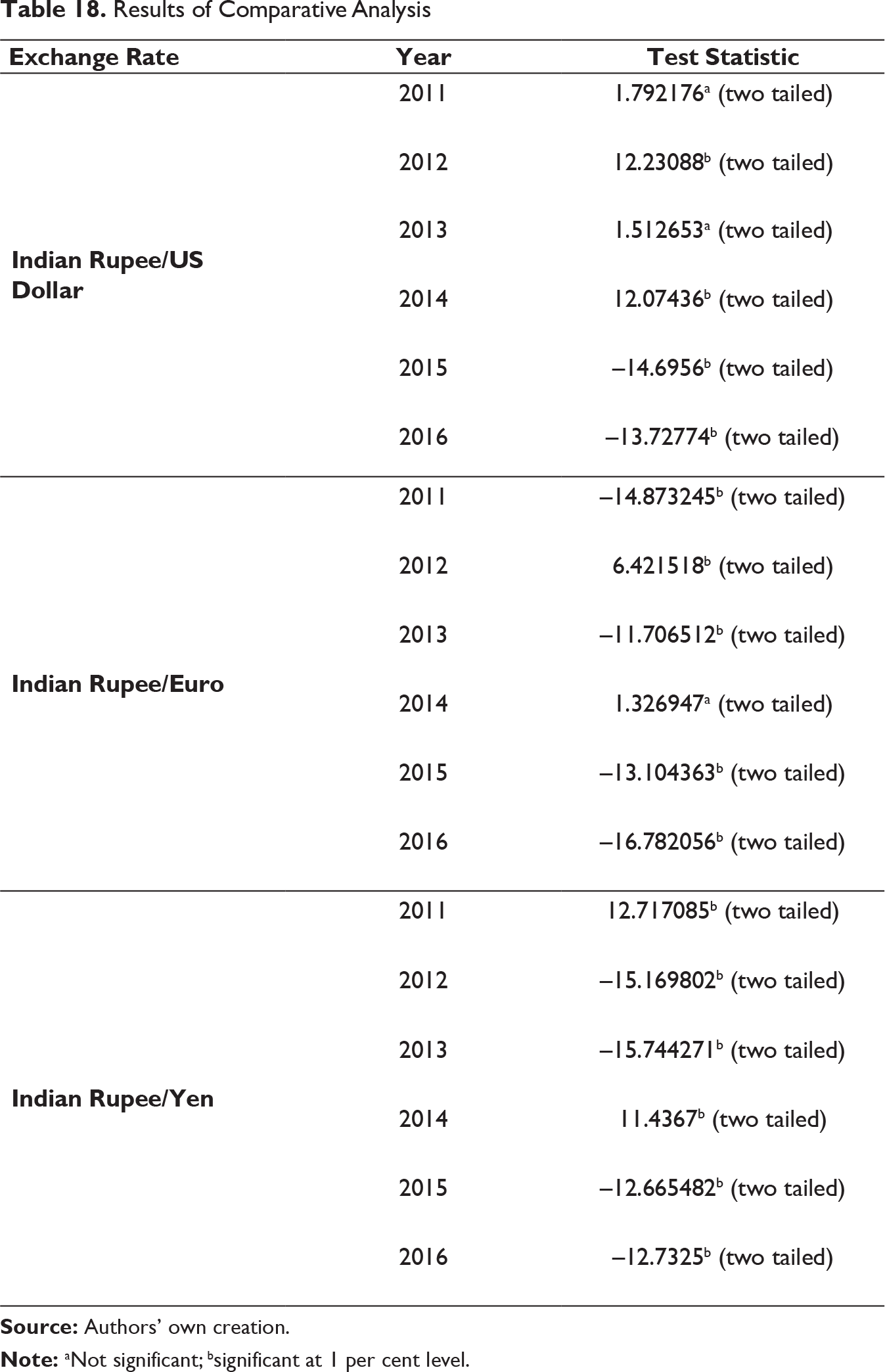
Although it is evident that both MODWT–RF and MODWT–bagging generate good predictions, it may be observed from Table 18 that there exists significant difference between their predictive performances. Total 18 experiments have been performed to assess the utility of both frameworks in predicting the respective exchange rates. In terms of MSE, MODWT–RF has yielded better forecasts as compared to MODWT–bagging on 10 occasions out of 18 cases (as indicated by negative significant test statistic). MODWT–bagging outperformed the former on five occasions. No significant difference in performance of two frameworks is observed in three instances (Indian rupee/US dollar in 2011 and 2013 and Indian rupee/euro in 2014).

Conclusion

This paper proposes a prediction framework of three different exchange rates, namely Indian rupee/US dollar, Indian rupee/euro and Indian rupee/Japanese yen during 2011–2016, by first decomposing each aggregate exchange rate series by MODWT using Haar wavelets and then aggregating the forecast of each sub-series to obtain the forecast values. For specifying the functional form between dependent and independent variables, an understanding of the time series data on exchange rates was undertaken through fractal investigation. Once the presence of persistence was observed in the time series, lagged values of the dependent variable were chosen as independent variables. The results indicate that both MODWT–RF and MODWT–bagging generated good predictions of the exchange rates.

References

Baetaens

D. J. E.

Van Den Berg

W. M.

Vaudrey

(1996). Market inefficiencies, technical trading and neural networks. In Dunis

(Ed.), Forecasting financial markets, financial economics and quantitative analysis (pp. 245–260). Chichester, England: John Wiley & Sons.

Balassa

(1964). The purchasing power parity doctrine: A reappraisal. Journal of Political Economy , 72(6), 584–596.

Bellgard

C. D.

(1998). Forecasting foreign exchange rates for profit (Unpublished honours dissertation supervised by Dr P.S. Goldschmidt). Department of Information Management and Marketing, the University of Western Australia, Perth.

Bellgard

Goldschmidt

(1998). Forecasting foreign exchange rates: Random walk hypothesis, linearity and data frequency. Retrieved 24 July 2017, from http://citeseerx.ist.psu.edu/viewdoc/download?doi=10.1.1.200.2574&rep=rep1&type=pdf

Breiman

(1996). Bagging predictors. Machine Learning , 24(2), 123–140.

Breiman

(2001). Random forests. Machine Learning , 45(1), 5–32.

Caves

R. E.

Jones

R. W.

(1981). World trade and payments: An introduction (3rd ed.). Boston and Toronto: Little Brown and Company.

Chaudhuri

T. D.

Ghosh

(2016). Artificial neural network and time series modelling based approach to forecasting the exchange rate in a multivariate framework. Journal of Financial and Insurance Management , 1(5), 92–123.

Dornbusch

(1980). Open economy macroeconomics . New York, NY: Basic Books.

10.

Fleming

J. M.

(1962). Domestic financial policies under fixed and floating exchange rates. Staff Papers (IMF), 9, 369–379. doi:10.2307/386609

11.

Gençay

Selçuk

Whitcher

(2001). An introduction to wavelets and other filtering methods in finance and economics . London, UK: Academic Press.

12.

Ghosh

Chaudhuri

T. D.

(2016). Understanding and forecasting stock market volatility through wavelet decomposition, statistical learning and econometric methods. Proceedings of Fourth International Conference on Business Analytics and Intelligence (ICBAI), December 19–21 . Bangalore, India.

13.

Hurst

H. E.

(1951). Long-term storage capacity of reservoirs. Transactions of the American Society of Civil Engineers , 116(1), 770–808.

14.

Kaashoek

J. F.

Van Dijk

H. K.

(2002). Neural network pruning applied to real exchange rate analysis. Journal of Forecasting , 21(8), 559–577.

15.

Khandelwal

Adhikari

Verma

(2015). Time series forecasting using hybrid ARIMA and ANN models based on DWT decomposition. Procedia Computer Science , 48(1), 173–179.

16.

Krueger

(1983). Trade and employment in developing countries, synthesis and conclusions . Chicago, US: The University of Chicago Press.

17.

Lebaron

(1999). Technical trading rule profitability and foreign exchange intervention. Journal of International Economics , 49(1), 125–143.

18.

Lemmens

Croux

(2006). Bagging and boosting classification trees to predict churn. Journal of Marketing Research , 43(2), 276–286.

19.

Liu

Wang

(2013). Comparison of random forest, support vector machine and back propagation neural network for electronic tongue data classification: Application to the recognition of orange beverage and Chinese vinegar. Sensors and Actuators B , 177(1), 970–980.

20.

Mandelbrot

(1972). Statistical methodology for non-periodic cycles from the co-variances of R/S analysis. Annals of Economics and Social Measurement , 1(3), 189–196.

21.

Mandelbrot

Wallis

(1968). Noah, Joseph and operational hydrology. Water Resources Research , 4(5), 909–918.

22.

Meade

James E.

(1951). The theory of international economic policy (Vol. 1: The Balance of Payments). London and New York, NY: Oxford University Press.

23.

Meade

James E.

(1955). The theory of international economic policy (Vol. 2: Trade and Welfare). London and New York, NY: Oxford University Press.

24.

Mundell

R. A.

(1963). Capital mobility and stabilization policy under fixed and flexible exchange rates. The Canadian Journal of Economics and Political Science , 29(4), 475–485.

25.

Ramsey

J. B.

Zhang

(1997). The analysis of foreign exchange data using waveform dictionaries. Journal of Empirical Finance , 4(4), 341–372.

26.

Samuelson

(1964). Theoretical notes on trade problems. Review of Economics and Statistics , 46(2), 145–154.

27.

Septiarini

T. W.

Abadi

A. M.

Taufik

M. R.

(2016). Application of wavelet fuzzy model to forecast the exchange rate IDR of USD. International Journal of Modeling and Optimization , 6(1), 66–70.

28.

Shmilovici

Kahiri

Ben-Gal

Hauser

(2009, March). Measuring the efficiency of the intraday forex market with a universal data compression algorithm. Journal of Computational Economics , 33(2), 131–154.

29.

Simidjievski

Todorovski

Dzeroski

(2015). Predicting long-term population dynamics with bagging and boosting of process-based models. Expert Systems with Applications , 42(22), 8484–8496.

30.

Tao

(2006). A wavelet neural network model for forecasting exchange rate integrated with genetic algorithm. International Journal of Computer Science and Network Security , 6(8A), 60–63.

31.

Wong

W. C.

Lui

(2003). Modelling and forecasting by wavelets, and the application to exchange rates. Journal of Applied Statistics , 30(5), 537–553.

32.

Xie

Ngai

E. W. T.

Ying

(2009). Customer churn prediction using improved balanced random forests. Expert Systems with Applications , 36(3), 5445–5449.

33.

Wang

Lai

K. K.

(2005). Adaptive smoothing neural networks in foreign exchange rate forecasting. In Sunderam

V. S.

van Albada

G. D.

Sloot

P. M. A.

Dongarra

(Eds.), Computational Science—ICCS 2005 (Vol. LNCS 3516, pp. 523–530). New York, NY: Springer.

34.

Zhang

G. P.

Berardi V.

(2001). Time series forecasting with neural network ensembles: An application for exchange rate prediction. Journal of the Operational Research Society , 52(6), 652–664.

35.

Zhang

(1994). Non-linear predictive models for intra-day foreign exchange trading. Intelligent Systems in Accounting, Finance and Management , 3(4), 293–302.

36.

Zheng

Caixin

Jian

Qing

Weigen

(2011). Entropy-based bagging for fault prediction of transformers using oil-dissolved gas data. Energies , 4(8), 1138–1147.

Fractal Investigation and Maximal Overlap Discrete Wavelet Transformation (MODWT)-based Machine Learning Framework for Forecasting Exchange Rates

Abstract

Abstract

Keywords

Introduction

Objective

Related Work

Research Methodology

Analysis on Data

Results and Analysis

Characteristics of Indian Rupee/US Dollar Rate over the Years

Characteristics of Indian Rupee/Euro Rate over the Years

Characteristics of Indian Rupee/Yen Rate over the Years

Results of Fractal Inspection

Descriptive Statistics of Hurst Exponent, FDI and CN

Forecasting Performance of RF on Indian Rupee/US Dollar Rate (Training Dataset)

Forecasting Performance of RF on Indian Rupee/US Dollar Rate (Test Dataset)

Forecasting Performance of RF on Indian Rupee/Euro Rate (Training Dataset)

Forecasting Performance of RF on Indian Rupee/Euro Rate (Test Dataset)

Forecasting Performance of RF on Indian Rupee/Yen Rate (Training Dataset)

Forecasting Performance of RF on Indian Rupee/Yen Rate (Test Dataset)

Forecasting Performance of Bagging on Indian Rupee/US Dollar Rate (Training Dataset)

Forecasting Performance of Bagging on Indian Rupee/US Dollar Rate (Test Dataset)

Forecasting Performance of Bagging on Indian Rupee/Euro Rate (Training Dataset)

Forecasting Performance of Bagging on Indian Rupee/Euro Rate (Test Dataset)

Forecasting Performance of Bagging on Indian Rupee/Yen Rate (Training Dataset)

Forecasting Performance of Bagging on Indian Rupee/Yen Rate (Test Dataset)

Results of Comparative Analysis

Conclusion

References

Descriptive Statistics of Hurst Exponent, FDI and C_N