




Abstract
In recent times there has been an increasing level of debate whether patterns do exist in equity market movements and whether they can be predicted. In order to overcome the shortcomings of traditional time series models, we have focused our study on the application of non-parametric paradigms like stacked multi-layer perceptrons (MLP), long short term memory (LSTM), gated recurrent unit (GRU), bidirectional long short term memory (BLSTM) and gated bidirectional recurrent unit (BGRU) on three NSE listed banks to predict short term stock price, and compared their performance with a shallow neural network benchmark. We have predicted equity ‘Close Prices’ five minutes into the future, using a sliding window approach and have observed that average error in predictions of MLP, LSTM, GRU, BLSTM and BGRU models, varied between 0.09% and 0.1%, indicating their superior performance with regard to benchmark baseline of 0.88%. We have used the aforementioned predictions to determine price trends, which successfully outperformed the random walk baseline accuracy of 50%.
Introduction
A sound prediction model of equity market movements can become the cornerstone of any successful stock trading strategy. Prior knowledge of the bullish or bearish tendency of the market is indispensable for achieving optimum asset allocation. Since a large volume of capital is traded in the stock market, a framework that can model the movements with a certain threshold reliability can realize large financial gains for the investor and also enable regulators of the market to plan corrective measures, in extreme scenarios.
In addition, another driving force for conducting this work is the rising levels of scepticism about Fama’s (1965) efficient market hypothesis (EMH) and Malkiel’s (1985) random walk theory. The criticism of EMH have led to the development of inefficient market hypothesis (IMH), which can be traced back to Grossman (1976), and Grossman and Stiglitz (1980). These literatures claim the existence of efficient markets to be impossible. Andrew Lo’s (2004) adaptive market hypothesis, adds traction to the IMH by claiming that markets are driven by the fear and greed of the participants rather than rationality alone, investors do not have fully ‘rational expectations’, but are driven by behavioural biases.
Traditional time series techniques had been extremely instrumental in modelling stock prices especially in the pre-machine learning (ML) era. Popular models like auto regressive conditional heteroscedastic (ARCH) methods (Engle, 1982) and auto regressive moving average (ARMA) (Box et al., 2015), or an auto regressive integrated moving average (ARIMA) assume equity prices to have a linear mathematical framework, whereas in reality stock market is a dynamically evolving non-linear framework. This has limited the ability of time series models to forecast prices. Machine learning models like support vector machines (SVM) (Suykens & Vandewalle, 1999), ensemble learning and artificial neural networks (ANN) can capture non-linear pattern in stock prices, without using any prior model assumptions. However, researchers implementing SVMs and other conventional ML models have observed that for small to moderate sized data-sets, having a few thousand points, ANNs can perform at par with ML models. They have generally exhibited overall superior performance than its ML counterparts with larger data-sets, having several thousands to millions of data points, which is our case using high frequency trading (HFT) data. This has propelled us to deep dive with ANNs like MLP and RNNs to present a comparative understanding about their efficacy in modelling stock prices.
The study required an enormous amount of review of both machine learning algorithms and financial theories. We did a detailed review of MLP (Gardner & Dorling, 1998), LSTM (Gers et al., 1999), GRU (Chung et al., 2014), BLSTM (Graves & Schmidhuber, 2005) and BGRU (Zhao et al., 2017). These expositions revealed to us the underlying mechanics of the algorithms which was found to be essential in the problem formulation. Application of deep learning in finance was explored through the works of Heaton et al. (2017), which helped us to understand the advantages of deep learning models over traditional ones. Zheng and Jin (2017) highlighted that although NN and SVM can model non-linearity, their performances were not satisfactory with respect to linear models. One of the potential reasons for sub-optimal results was that the models were being trained on smaller data-sets, which served as a bottle neck for the non-linear models to realize their true predictive power. It served as a guideline for us to train the models on larger data-sets. Naeini et al. (2010) predicted inter day stock price prediction and observed that memoryless networks like MLP outperformed time series networks like LSTM. We followed a similar line of action but experimented with a wider variety of memory based neural networks. Liu et al. (2019) applied a novel approach by first de-noising the data and then applying LSTM on it. Although this methodology helps in improving the accuracy of a single LSTM model, it makes the approach computationally expensive. Recent studies in Indian context like Khare et al. (2017) have found similar results as Naeini et al. (2010). They have performed a heuristic feature engineering process, to identify key technical indicators that can help improve the predictive accuracy. Selvin et al. (2017) have found that convolutional neural network (CNN) have outperformed memory based networks like LSTM and RNNs.
We have extended the work of Khare et al. (2017) and Selvin et al. (2017) through our experiments, with a fundamental difference of not performing feature engineering. Our assumption is that NNs can identify latent non-linear patterns in the data; therefore, the technical indicators identified from a feature engineering process might be implicitly taken into account. In addition, since stock market is a dynamically evolving framework, a set of technical indicators that might be important in making predictions today might not be relevant to that extent in a different time period under consideration. Selvin et al. (2017) trained their models for 1000 epochs, which can lead to a significantly higher training time. We took this into account and trained our models for less than 50 epochs, with comparable error rates.
Prediction Philosophy
This section provides an outline of specific time horizon of prediction chosen for this paper and mentions the NN techniques to be adopted. In the later half we shed light on the logical framework used to map the input to the targets (Data preparation—model building; and Optimization—performance evaluation).
Methodology
Stock price prediction can be grouped into three categories:
Short term prediction—spanning over seconds to weeks Medium term prediction—spanning over months to a couple of years Long term prediction—spanning beyond two years
Lot of research has been already devoted on medium term and long term stock price predictions yielding more than 70% accuracy, on many occasions. This paper has focused on short term stock price prediction since this area has not witnessed models that can consistently predict price movements with more than 60% accuracy. Some attempts on short term price prediction has been made using NNs like multi-layer perceptron (MLP), convolutional neural network (CNN), recurrent neural network (RNN). However in many of these NN approaches researchers have attempted to predict the stock prices, instead of price movements, yielding much better accuracy than their conventional machine learning counterparts. An NN architecture directly modelling stock prices might produce a small mean error creating a false impression of superior predictive performance but it might be actually exhibiting poor accuracy in predicting market movements, especially when price movements are relatively smaller in magnitude. Taking account of this drawback our paper aims to design a two-pronged strategy which sets up a regression approach to forecast future stock prices, and subsequently filter in the percentage of predictions which are in the correct direction. We have used high frequency trading (HFT) data as input and extended the existing MLP and RNN architectures into deep neural networks (DNN), stacked GRU, stacked LSTM, stacked BLSTM and stacked BGRU, to perform a comparative analysis of the model performances.
Proposed Approach
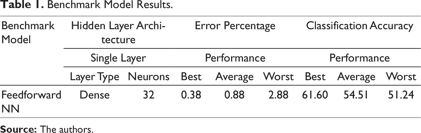
Harnessing the desired performance from a deep learning architecture can be a daunting exercise. Numerous trials had to conducted with different configuration of model parameters like layer width, model depth, activation function, regularization features, input data and batch sizes, before finalizing the architectures. In this section the reader will be walked through the steps adopted in tackling the stock price prediction problem. The data-set consists of a highly granular second-by-second stock price data of three prominent financial institutions listed in National Stock Exchange (NSE), namely ICICI Bank, Axis Bank and Yes Bank for a one month period in November 2017. In this paper we have used historical data which has information on the date-time stamp, open price, high price, low price and close price for each second. The data was originally extracted from order book. The prices varied from 300 to 335 for ICICI Bank, 290 to 330 for YES Bank and 520 to 570 for AXIS Bank. A closer examination revealed that the price data was not recorded for each second, since no trade had been conducted in those seconds. To filter out the missing points, we appropriately down-sampled the data at every 30 seconds interval, providing the models with approximately 15000 data points for each stock. The data-set was normalized and partitioned into training, validation and test set. The section delves deeper into the aspect of data wrangling and partitioning. The models were build and optimized on ICICI Bank data-set. The same models were freshly retrained and tested on AXIS Bank and YES Bank data-sets without any further adjustments to get an idea of the generalized performance. The approach employs a sliding window technique for forecasting future close prices. We used a 60-minute window of past price data (open, high, low, close), sampled at every 30-second interval to predict the close price 5 minutes in the future. A shallow feedforward NN model with one hidden layer was used as a benchmark. This was the best way to ensure that any further non-linearity we introduced through advanced models was justified, and produced better results. Five different NN models namely MLP, LSTM, GRU, BLSTM, BGRU, were built using Keras open-source package with Tensorflow backend in Python environment. The section ‘Model Architecture’ gives a deeper insight into the deep learning models applied in this paper. Extensive trials were performed before finalizing a model which had training and validation set, mean absolute error (MAE) converging to comparable values within acceptable error limit. This was monitored by plotting training and validation losses versus a predefined number of epochs. It was observed that for the better models, training and validation losses reduced to minimum values within 20 epochs, after which validation losses started to increase indicating the model had started to overfit. The trained model was evaluated on the test data-set yielding test MAE from which the error percentage (ep) was calculated (refer to the section ‘Prediction Analyses’). As pointed before in the section ‘Methodology’, a closely fitting prediction model does not necessarily imply that it will exhibit equivalent performance in forecasting close price movements (up or down). Thus, we implemented a classification strategy which took into consideration close prices at the current time step, predicted close prices at a future time step where the prediction was to be made and the actual close prices at the corresponding future time step; to create a prediction movement vector and an actual movement vector which stored predicted and actual price movements from the current time step, respectively. A 2×2 classification matrix between predicted movement and actual movement was created to distil the information from price movement vectors into a summary of correct (predicted-up, actual-up and predicted-down, actual-down) and incorrect (predicted-up, actual-down and predicted-down, actual-up) percentage of price movement predictions.
Model Architecture
This paper employs five deep learning architectures MLP, GRU, LSTM, BLSTM and BGRU. We start with the basic intuition of what a neural network is and gradually build on that to explain the advanced models.
Fundamentals of a Neural Network
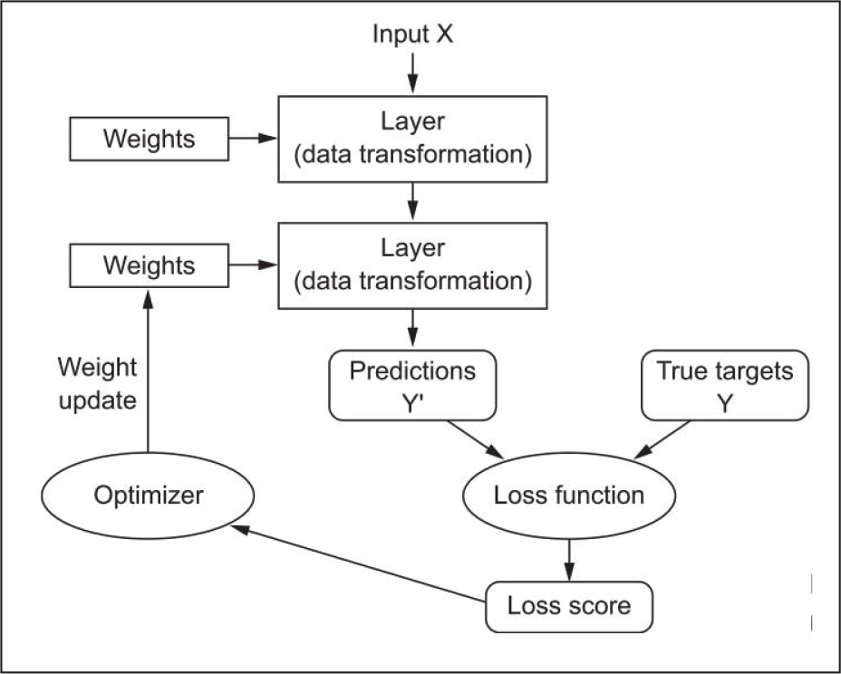
Haykin (1994) aptly defines a neural network as a massively parallel distributed processor that has a natural propensity for storing experiential knowledge and making it available for use. It resembles the brain in two respects: Knowledge is acquired by the network through a learning process. Inter-neuron connection strengths known as synaptic weights are used to store the knowledge. The anatomy of an NN consists of the following principal components (Figure 1).
The Input Data and Corresponding Targets
The mapping of input-target takes place through a series of non-linear transformations implemented by the layers. Learning is implemented by a backpropagation algorithm which adjusts the layer weights in a direction, that reduces the loss score as the model encounters more examples from the training set. This process it iterated over an appropriate number of epochs such that the loss function is minimized and the model does not start to overfit.
Multi-layer Perceptron
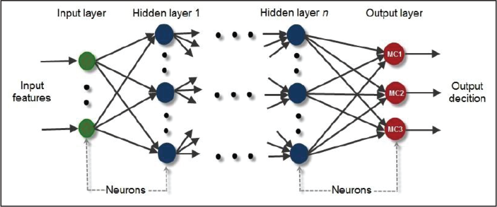
A feedforward NN is a fundamental form of ANN where information flows in forward direction from the input layer to the output layer, through hidden layer(s) (Figure 2). Each layer, receives it’s input from the previous layer, learns abstract features from it by projecting the input in a hypothetical space and feeds its output forward, to the next layer. The nodes in this network do not have cyclical connections. A MLP is a special class of feedforward NN with an input layer, an output layer and one or more hidden layers, using some non-linear activation function(s).
Recurrent Neural Network
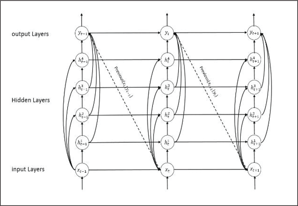
Recurrent Neural Network (RNN) is basically a type of NN that has an internal loop. Chung et al. (2014) describes that RNN processes a sequence of arbitrary length by recursively applying a transition function to its internal hidden state for each symbol of the input sequence (Figure 3). The activation of the hidden state at time-step t is computed as a function of the current input symbol x
t
and the previous hidden state h
t
-1. Mathematically, it can be represented as:

such that Φ is activation function, W is input to hidden layer weight matrix, and U is state to state recurrent weight matrix.
RNNs suffer from vanishing gradient and exploding gradient problems, making it difficult for gradient descent algorithms to train them and capture long term temporal dependencies. Researchers have been able to overcome this hurdle by developing a modified version of RNNs, namely gated RNN (GRNN) that uses a gated memory system which controls the flow of information over long periods of time. In this paper two types of GRNNs have been used, namely LSTM and GRU, which have similar network architectures like RNNs, except that each RNN unit replaced by a LSTM and GRU unit, respectively.
A typical Feedforward MLP.
An Unrolled Representation of a Stacked RNN.
Long Short Term Memory
LSTM was proposed by Hochreiter and Schmidhuber (1997). In addition to having standard units of a RNN, each LSTM unit contains a memory cell which can store additional important input features in the memory for longer time periods. A set of logic gates is used to control the flow of information through the memory. The functioning of a typical LSTM unit is summarized as follows (Figure 4).






Gated Recurrent Unit
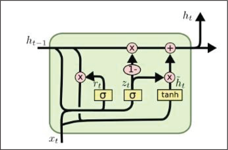
GRU was proposed by Chung et al. (2014). It has a similar line of functioning like LSTM but has a simplified configuration with fewer logic gates. They are relatively new as compared to LSTM, and are found to deliver performance at par with them, with a higher computational efficiency. It has a gating mechanism that controls flow of information (input features) but does not use a memory cell unlike LSTM. The functioning of a typical GRU unit is summarized as follows (Figure 5).




Bidirectional Recurrent Neural Networks
Bidirectional RNN (BRNN), was introduced by Schuster and Paliwal (1997). This technique enables the network to have past and future information about the data sequence at each time step. Basically it connects two hidden layers of opposite directions to the same output layer, giving it access to past and future states. The regular RNN neuron is split in two directions—one for future states (forward direction), another for past states (backward direction). Outputs of these two states are not connected to the input states of opposite direction (Figure 6). Since regular RNN units form the basic building blocks of BRNNs, vanishing gradient and exploding gradient problems persist here as well. To eradicate this issue we have experimented bidirectional LSTM (BLSTM) and bidirectional GRU (BGRU) architectures.
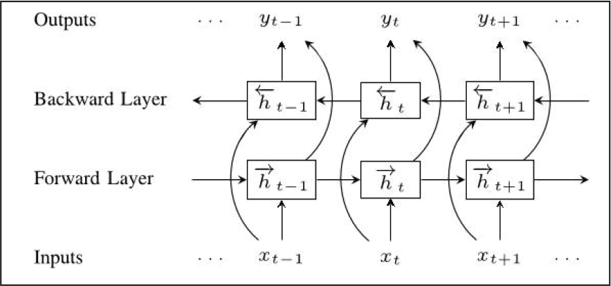
BLSTM and BGRU, both possess the capability of learning past and future long term temporal dependencies, unlike conventional BRNNs. Their network architectures are similar to BRNNs, except that it employs two directional LSTM and GRU neurons respectively, instead of two directional RNN neurons. BLSTMs and BGRUs have exhibited better predictive performance than their unidirectional counterparts (LSTM and GRU respectively), especially in speech recognition and language translation domains.
Results and Analysis
In this section, we touch upon the data wrangling and partitioning approaches employed and move on to the dual perspective from which have tried to approach the prediction problem. In the later stages of the section we interpret the results obtained from the experiments.
Data Preparation
The models were trained on the first 11000 data points, validated on next 2000 data points (11001–13000) and tested on the remaining 2000 points (13001–15000). We fed the data in the model, in batches. After repeated trials with varying batch sizes, a batch size of 128 was fixed as it was yielding the best result. NNs face difficulty in processing un-normalized data, severely impeding their learning rate, thereby creating a hindrance for the architecture in realizing their full potential. Each time series of the particular stock price data under consideration was on a different scale. Thus before feeding the data to the models, each time, series was normalized independently so that they could attain smaller values in a similar scale.
Feature Selection
The objective of this paper was to demonstrate the accuracy of advanced deep learning models in predicting future stock prices and their movements. We have avoided use of any technical indicators and restricted ourselves to basic features available from historical stock price data (open, high, low and close), since advanced technical indicators can certainly boost the model performance but it will hinder us from understanding the sole power of the NN models.
Prediction Analyses
In this section the performance of NN models on ICICI Bank, YES Bank and AXIS Bank data-sets have been evaluated. To render a better clarity to the reader, the objectives behind conducting the experiments have been articulated below.
In the context of our work, model performance encapsulates a dual interpretation. Below, we crystallize the performance evaluation standpoints proposed in the section 2.2 ‘Proposed Approach’ for understanding the predictive power of a model.
Regression Perspective: Price Prediction
This approach aims to build a prediction curve that best fits the actual target curve. Performance metric used to evaluate the accuracy of fit is error percentage (ep), which can be mathematically represented as:

where ScaledTestMAE is de-normalized MAE of the test data-set calculated as follows:

std is standard deviation of training data-set and TestMean is mean close price of the de-normalized test data-set.
Classification Perspective: Trend Prediction
This approach considers the prices predicted from the regression model and distils all the correct trend predictions into a fraction of all the predictions made. Performance metric used to evaluate the accuracy of trend prediction is classification accuracy (CACC), which can be mathematically represented as:

Based on the above discussion we have evaluated model performances separately with respect to EP in the section ‘Stock Price Analysis’ and CACC in section ??
Benchmark Model Results.
Neural Network Architectures Used.

Stock Price Analysis
Comparison of Best, Average and Worst Case Percentage Errors in Predicted Close Price.
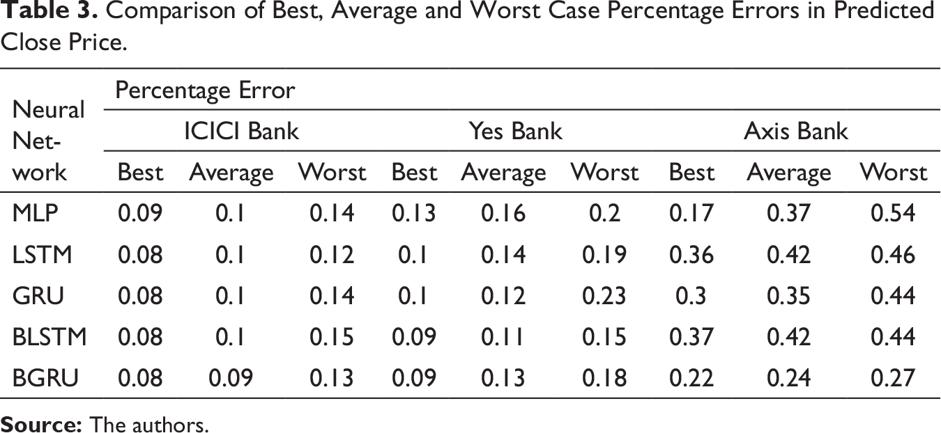
Once the supremacy of these models became evident, we retrained the same models on YES Bank and AXIS Bank data-sets and interpreted their performance as discussed below.
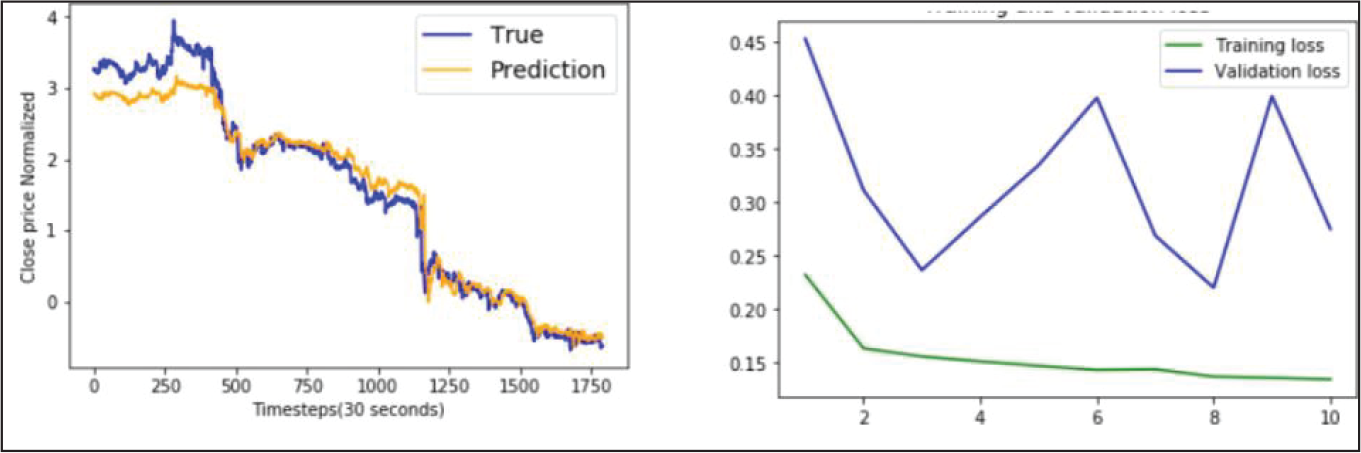
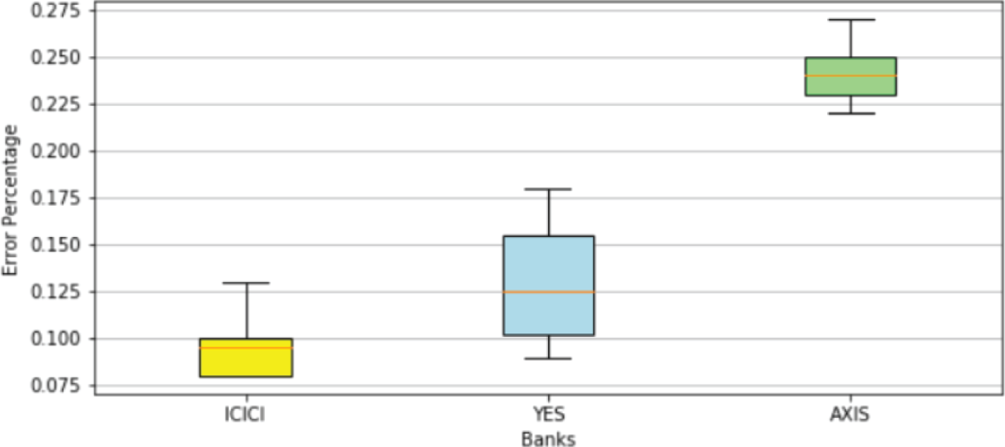
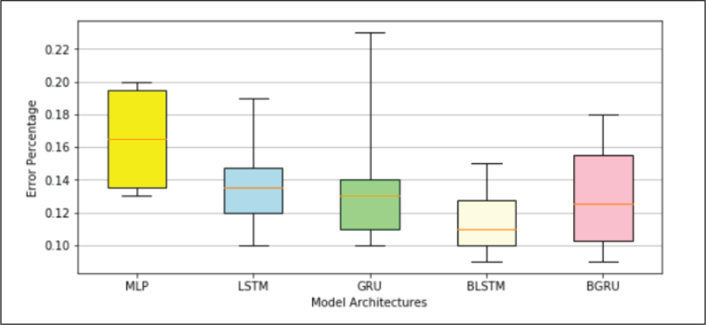
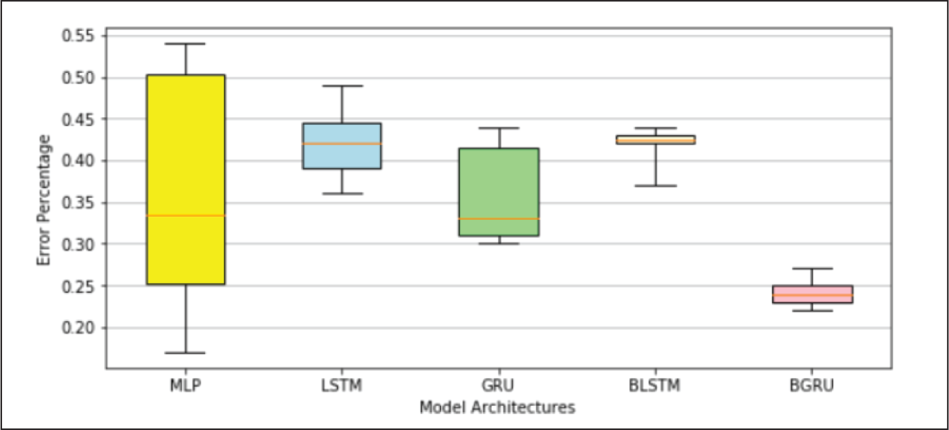
A closer examination of the model performances recorded in Table 3 indicates that error percentages of each type of NN architecture increased moderately for YES Bank data-set and significantly for AXIS Bank data-set. Appendix B.1 gives a better visual depiction of this behaviour, where for each NN model the range of errors recorded in the three data-sets were represented through box plots. It was noted that the average errors of all the models varied from 0.09% to 0.10% on ICICI Bank data-set, 0.11% to 0.16% on YES Bank data-set and 0.24% to 0.42% on AXIS Bank data-set. We investigated this variation further by examining the best case graphs of the predicted and actual prices on the test data, and corresponding training and validation losses from Appendix B.1. Inferences for each type of NN model on the three data-sets are as follows.
The inconsistency can be attributed to the fact that the set of features driving the stock prices for each of these banks are at least partially non-overlapping and also the corresponding common features might have different weights. As a consequence models trained and optimized on ICICI Bank data-set overfitted on YES Bank and AXIS Bank data-sets. ICICI Bank might have had a more complex set of latent patterns, whereas YES Bank and AXIS Bank might have had a simpler set of features which made the models too sophisticated for YES Bank and Axis Bank data-sets, and thus they started modelling the random noise.
An examination of average errors on each data-set yielded by the different models from Table 3 and box plots shown in Appendix B.2 revealed the following facts. YES Bank: The average errors of all the models varied from 0.11% to 0.16%. The higher error magnitude and variation was due to the fact that the models were not fine-tuned with respect to this data-set. BLSTM was the best and MLP was the worst performing model. GRU marginally outperformed LSTM, but exhibited a wider range, and again both these models were beaten by their bidirectional counterparts. BLSTM outperformed BGRU and was more consistent. AXIS Bank: The average errors of all the models varied from 0.24% to 0.42%. The higher error have been already explained above. BGRU was the best and LSTM was the worst performing model. Since the models were found to severely overfit this data-set, yielding unreliable performances, we refrain ourselves from drawing any further inference.
Stock Trend Analysis
Comparison of Best, Average and Worst Case Classification Accuracy in Predicted Close Price Movements.

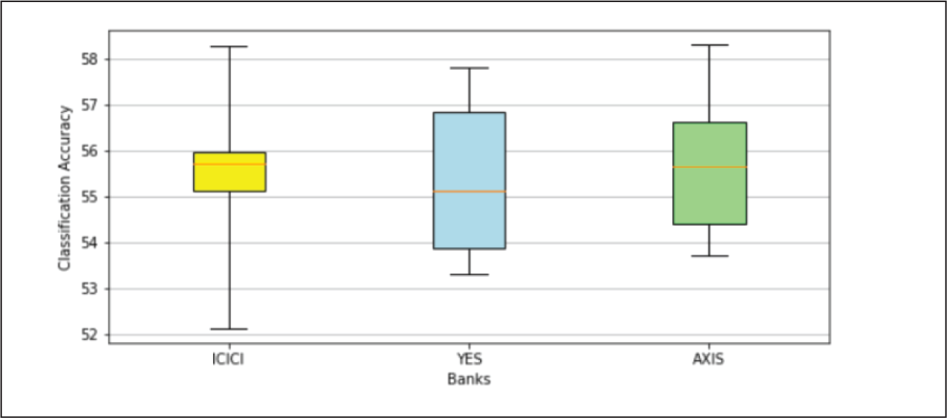
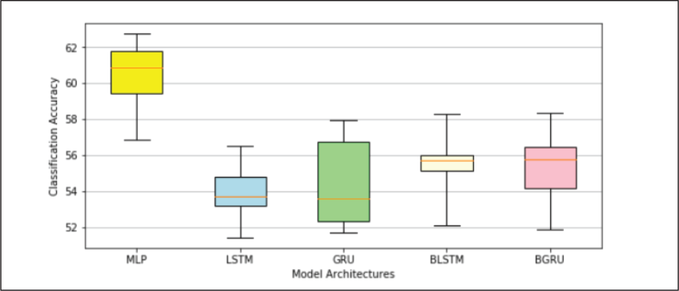
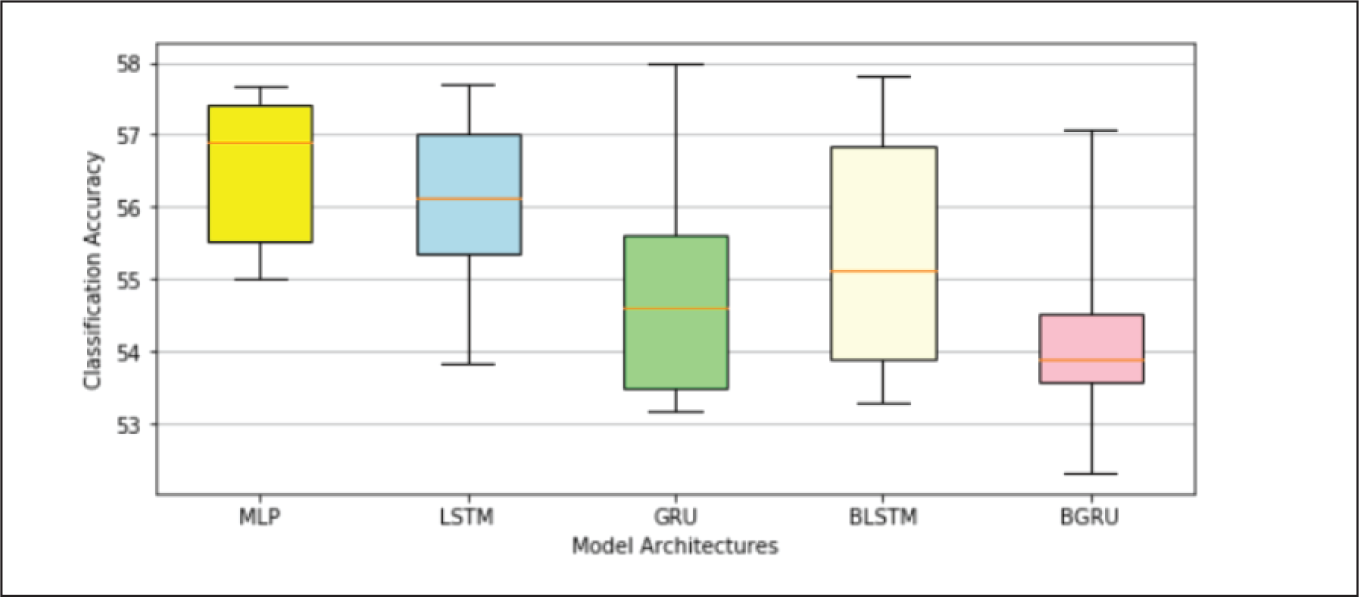
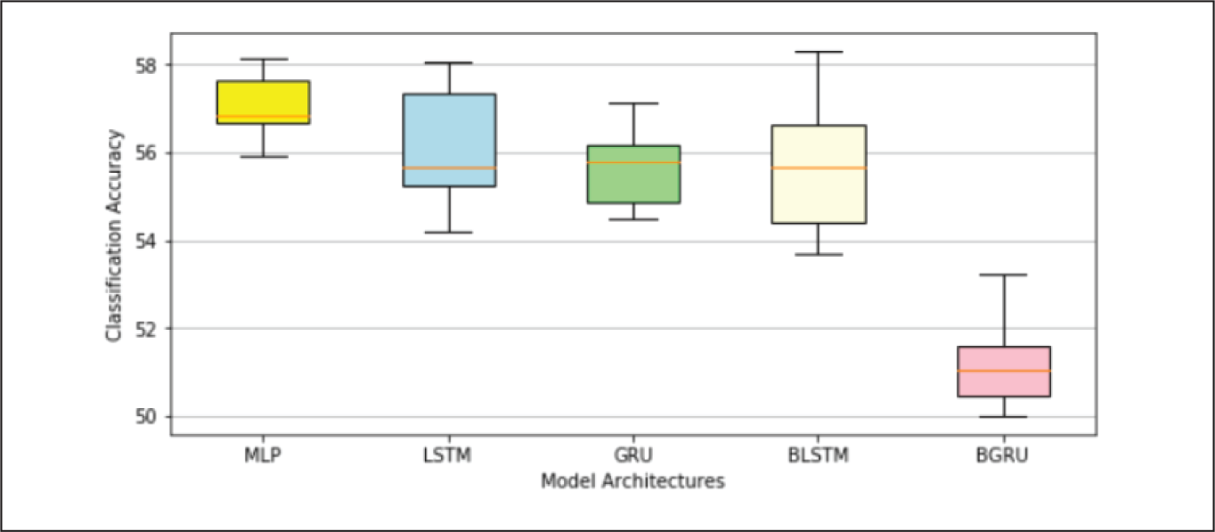
Table 4 and Appendix B.3 indicates that classification accuracies of MLP and BGRU models on ICICI Bank data-set were better than that on YES Bank and AXIS Bank data-sets, whereas other models described an opposite trend. The MLP model has consistently shown superior performance over other models on all the data-sets. Other models exhibited more random patterns possibly due to overfitting issues in YES Bank and AXIS Bank data, making it very difficult to rank them in a logical order. One has to perform a significantly higher number trials on these models to draw meaningful conclusions on their performance.
Table 4 and box plots shown in Appendix B.4 revealed the following facts, on classification accuracies, yielded by the different models on each data-set.
ICICI Bank: The average classification accuracies of all the models varied from 54.17% to 60.00%. MLP was the best and LSTM was the worst performing model, with GRU being marginally better than LSTM. BLSTM and BGRU outperformed their unidirectional counterparts, but were far from matching MLP performance.
YES Bank: The average classification accuracies of all the models varied from 54.11% to 56.54%. MLP was the best and BGRU was the worst performing model, with GRU being marginally better than LSTM. LSTM and GRU outperformed their bidirectional counterparts.
AXIS Bank: The average classification accuracies of all the models varied from 51.34% to 57.58%. MLP was the best and BGRU was the worst performing model. Due to severe model overfitting issues with this data-set, any deeper model performance evaluation might not be meaningful.
Conclusion
In this paper, we have designed five DNN models—MLP, LSTM, GRU, BLSTM and BGRU—to predict the short term stock prices values and their movements, five minutes into the future, for three stocks on the NSE. We found that the versatility of NN models cannot be taken for granted. The model architectures are very much a function of the data-set. Optimum networks for a particular data-set might require certain degree of adjustments for delivering equivalent results on other data-sets and keeping overfitting issues at bay. In this context we want to point out that models applied on AXIS Bank data-set grappled with severe overfitting problems, and therefore in the rest of this section, comments on model performances have been made primarily with respect to ICICI Bank and YES Bank, unless stated otherwise. One needs to remove overfitting issues from the AXIS Bank models to fully understand the implications of their results.
Based on experimental results cited in the section ‘Results and Analysis’, we can claim that NN models are certainly proficient in modelling highly non-linear time series stock data. From the perspective of price prediction, all the models were found to deliver nearly similar accurate results. However MLP models were found to deliver much better results than others in predicting price movements and overall emerged as the best model. This is primarily due to the fact that MLP only takes into account current information in making predictions, and is oblivious to patterns learnt from previous time steps, making them more agile in understanding the dynamic changes in the current window. Stock market is a highly dynamic machinery, especially in short term horizon, where the set of features driving the market might radically evolve from time to time in a non-periodic manner. LSTM, GRU, BLSTM and BGRU models consider long term dependencies which might actually become irrelevant in the current context, but since these models try to understand the present information through the prism of past dependencies, it actually creates hindrance in learning the current patterns and dynamics in the system, often leading into incorrect trend predictions. Similar behaviour was recorded by Selvin et al. (2017) (Liu et al., 2019) and Khare et al. (2017) (Graves & Schmidhuber, 2005).
Even though the MLPs exhibited high accuracy in predicting stock prices, their performance in predicting price trends were not encouraging, with the best trend prediction accuracy being 62.74%. This is somewhat contradictory since the best case graphs of ICICI Bank and YES Bank showed quite accurate fits, we had expected better results. We looked into the magnitude of price changes and observed that approximately 80% of the changes in successive time steps were less than 0.2 units, 40% of the changes were less than 0.1 units and 5% of the changes were greater than 1 unit. Thus a major fraction of the price variations were actually small fluctuations, which might not be significant for stock traders. It is therefore more practical to cluster the movements into different bands—say small, medium and large—as per the investor’s requirement and analyze the model performance separately in the relevant clusters, instead of the entire test set all at once. Our endeavours have certainly rendered evidence of the superior power of NNs in predicting stock prices. However this powerful weapon can become meaningless unless one points it in the right direction. We want to suggest possible areas of improvement in this work that can serve as a premise of future works in this domain: past price data may not be sufficient in making future predictions. Including advanced technical indicators in similar lines with those mentioned by Zheng and Jin (2017) (Hochreiter & Schmidhuber, 1997) can enhance the power of our models. However one has to take into account that many of the technical features are derived directly from historical data itself. Our complex algorithms might have already incorporated their effects, so significant improvements might not be certain. One should utilize market sentiment information to understand the forces that are more likely to drive prices in the near future to identify more important features. The importance of features can be objectively summarized using a feature importance index. One has to explicitly feed these models with the feature importance factors and explore further for better results. We had selected the best models through substantial manual trial and errors. However these models may not be the optimum networks in the entire search space since one has to experiment with almost all possible cases to arrive at such a conclusion. It might take an unrealistically high time for such experimentation even with advanced computing capabilities. A possible way to resolve this issue can be to reduce the search space through preliminary trial and errors and then explore the application of genetic algorithm in the simplified space.
Appendices
Appendix A. Best Case Graphs
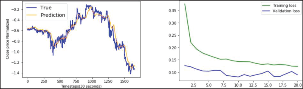
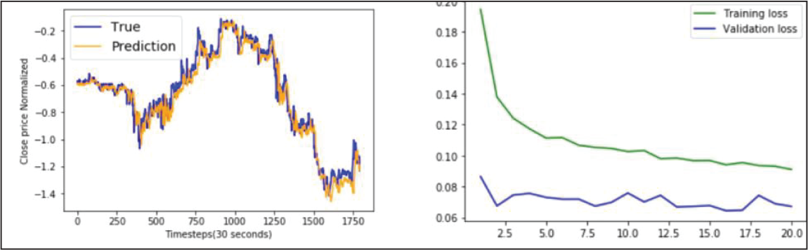
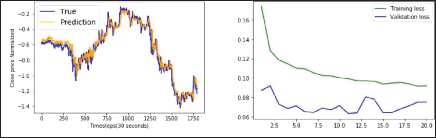
BLSTM Model Performance on ICICI Bank Data.
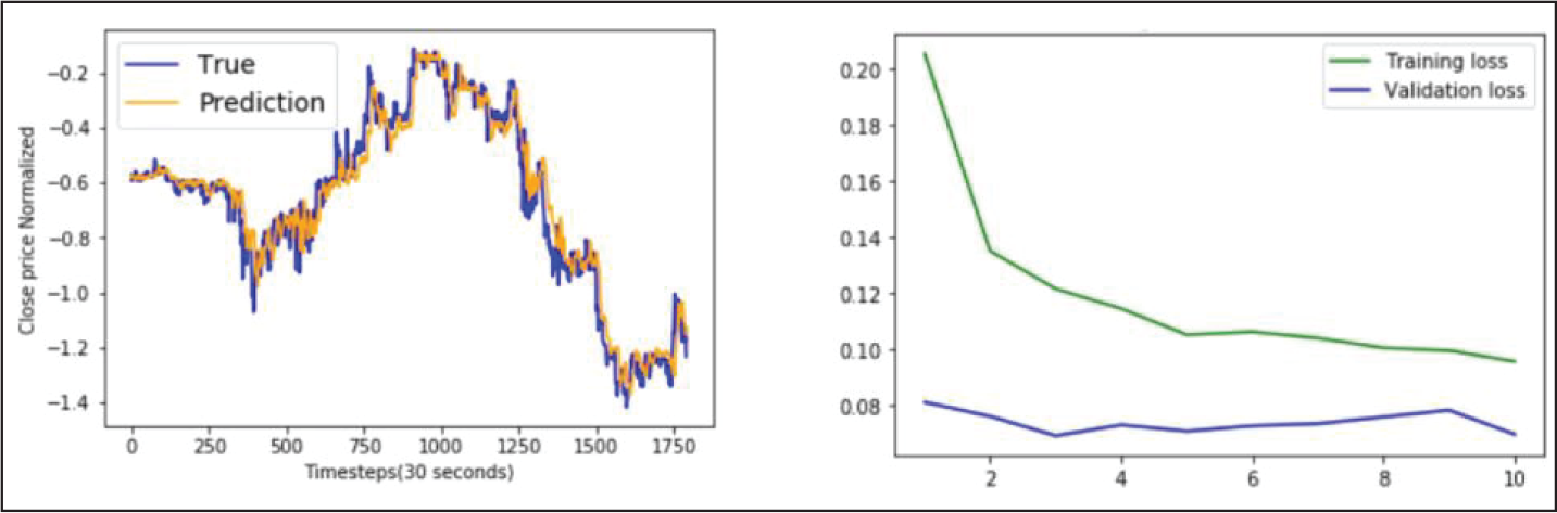
BGRU Model Performance on ICICI Bank Data.

MLP Model Performance on YES Bank Data.
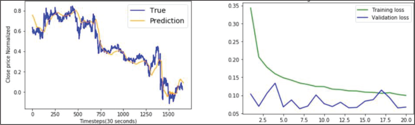
LSTM Model Performance on YES Bank Data.
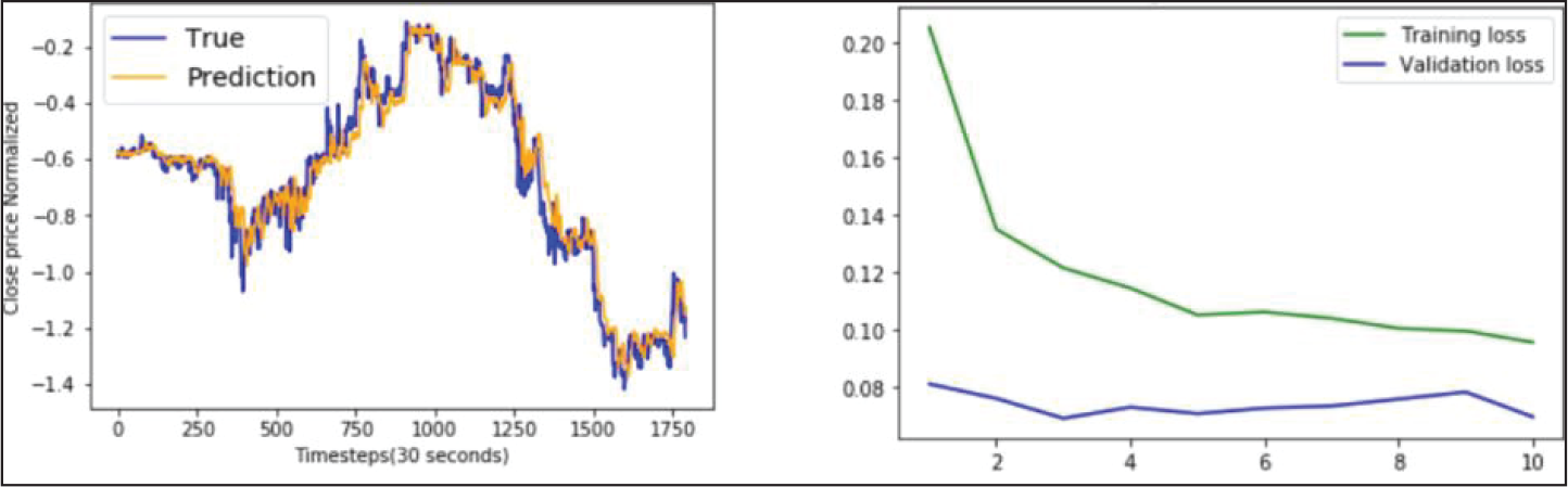
GRU Model Performance on YES Bank Data.
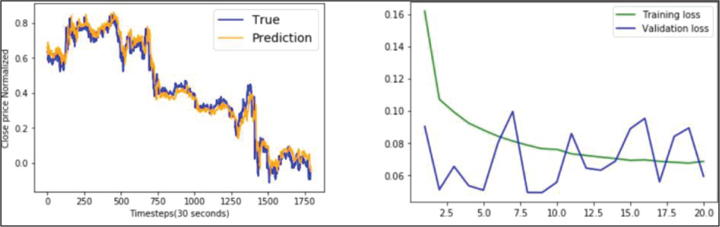
BLSTM Model Performance on YES Bank Data.

BGRU Model Performance on YES Bank Data.
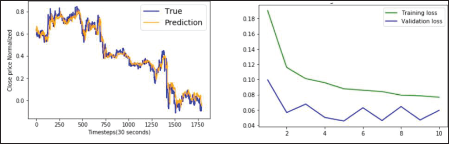
MLP Model Performance on AXIS Bank Data.

LSTM Model Performance on AXIS Bank Data.
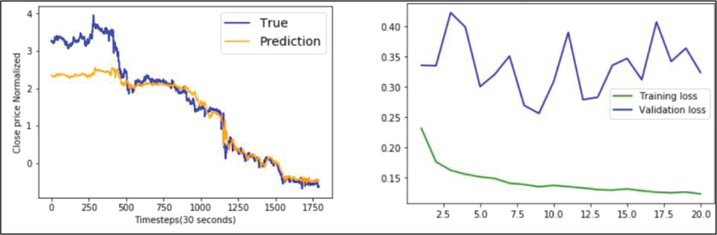
GRU Model Performance on AXIS Bank Data.

BLSTM Model Performance on AXIS Bank Data.

BGRU Model Performance on AXIS Bank Data.
Appendix B: Box-plots
MLP Model Performance.
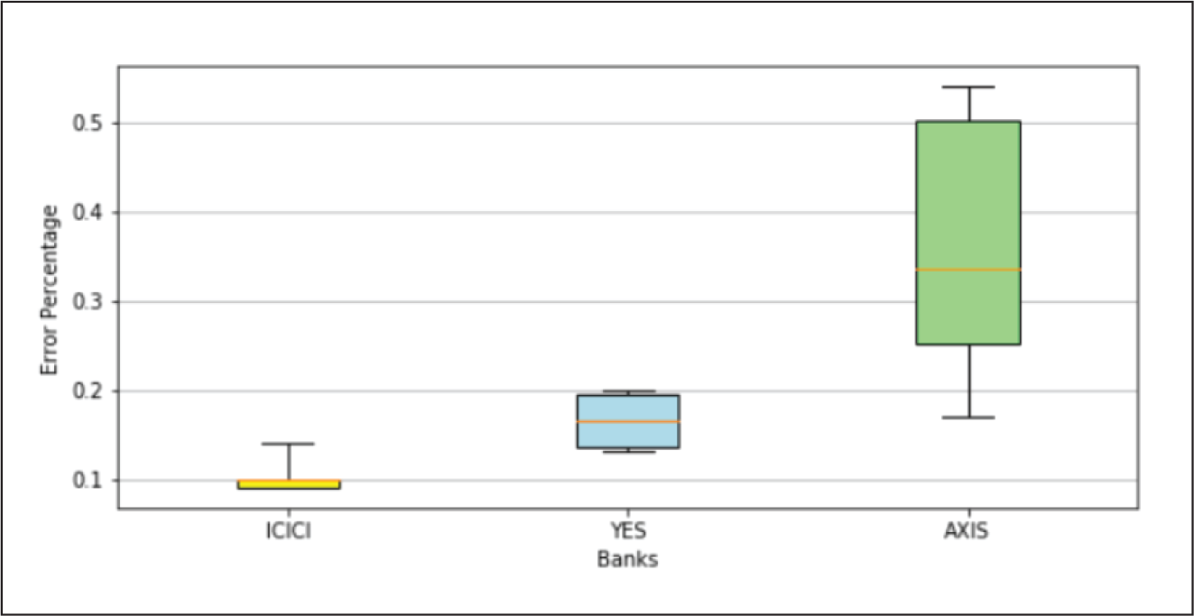
LSTM Model Performance.
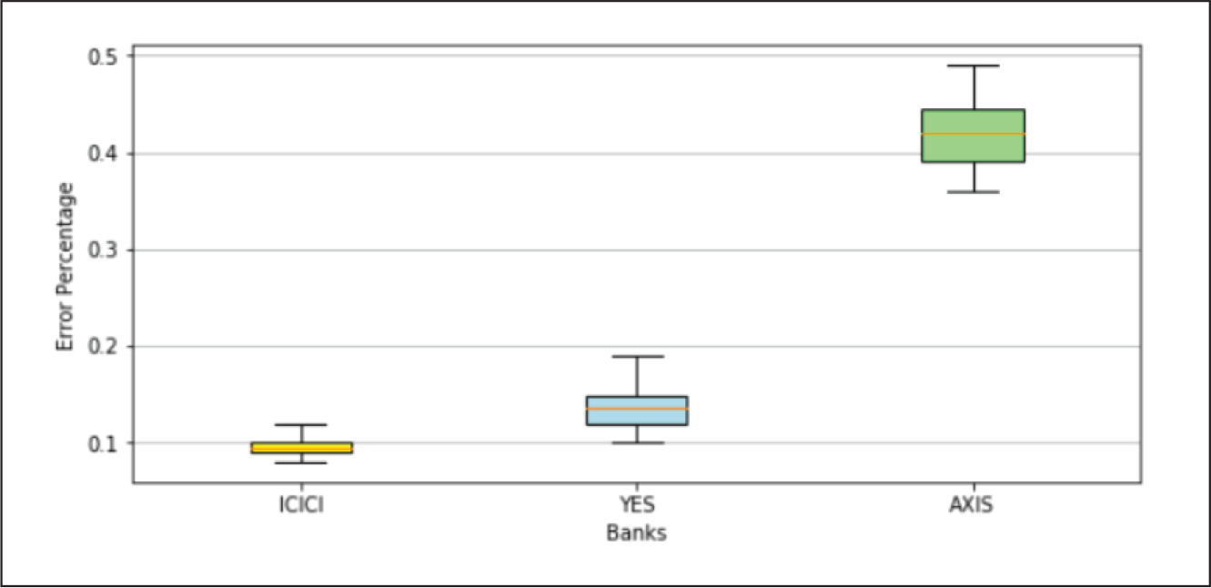
GRU Model Performance.

BLSTM Model Performance.
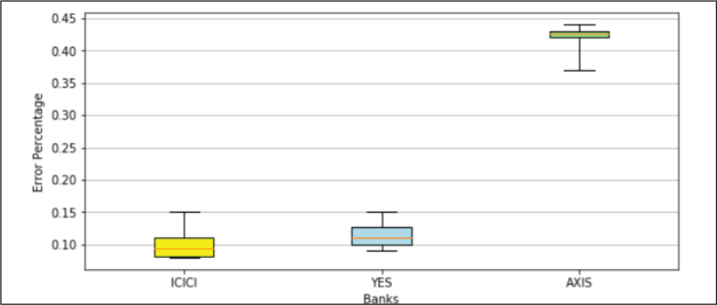
BGRU Model Performance.
Performance on ICICI Bank Data-Set.

Performance on YES Bank Data-Set.
Performance on AXIS Bank Data-Set.
MLP Model Performance.

LSTM Model Performance.

GRU Model Performance.

BLSTM Model Performance.
BGRU Model Performance.

Performance on ICICI Bank Data-Set.
Performance on YES Bank Data-Set.
Performance on AXIS Bank Data-Set.
Footnotes
Declaration of Conflicting Interests
The authors declared no potential conflicts of interest with respect to the research, authorship and/or publication of this article.
Funding
The authors received no financial support for the research, authorship and/or publication of this article.
