




Abstract
This paper derives a method of measuring the degree of collusion among the bidders in an open ascending repetitive price auction in agricultural commodity markets in India. This paper first derives the bidders’ behaviour’s theoretical structure and then a measure of collusion formation. Finally, the degree of the cartel has been computed using time series wholesale price data of potato and onion crops. This research’s findings are helpful for the study of the link between the supply of the agriculture commodity and the degree of collusion. Using the proposed method in this research, if the Agricultural Produce Market Committee (APMC) measures cartel for each market and publish periodically, it will help farmers choose the right market to sell the produce. The farmers would select the market where the degree of collusion is relatively lower. Identifying different small cartel groups at different times with respective to the supply of the agriculture commodity would help avoid the incidence of distress selling by farmers, which is the main hindrance in developing the farming community in India.
Introduction
In the agrarian economy of India, the low level of farm income has been a chronic and significant source of farm distress (Chand, 2017). Prices of agriculture commodities received by farmers are a significant determinant of farmers’ income (Beckman & Schimmelpfennig, 2015; Chand, 2012). Agricultural marketing in India is characterized by pervasive government intervention. The form of intervention has changed over time as per the requirements or reforms needed. For the upgradation of the marketing system and bringing about transparency in the price discovery and encouraging competition, the Ministry of Agriculture, Government of India, proposed a model act called Agricultural Produce Marketing Act in 2003. This act authorized the State governments to regulate marketing practices in the wholesale markets. The states set up regulated markets in every district where the farmers were to sell their produce. The fruits and vegetables have been kept outside of the purview of the APMC Act in different states of the country. There are about 2,477 principal regulated markets and 4,843 sub-market yards regulated by the respective APMCs in India. 1 This act helped the farmers by providing them with the market for producing, grading, and sorting minimum support prices (MSP) set up by the government and immediate payments (Acharya & Aggarwal, 2011).
In India, the agricultural market is characterized by many sellers and a small number of buyers. This phenomenon leads to cartelization by traders and the exploitation of farmers. One of the disturbing phenomena reported by some studies has been the cartelization by market functionaries such as traders and commission agents (Madhavan et al., 1994; Severová & Bendl, 2013). Cartelization is the formal organization of a group of producers or suppliers to control the competition by regulating or manipulating prices. The cartel uses many tactics to achieve its mission, such as reduced supply, price fixation, collusive bidding and market carving. Cartels have many disadvantages as they tend to increase the prices for the end consumer compared to market prices by restricting the supply. This discourage competition by increasing the barrier to market entry by controlling the resources. Many research has been done in order to understand the various aspects of cartelization. Connor (2005) studied the relationship between collusion and price dispersion, that is, how the price dispersion changes when cartelization occurs. He used four cartels to suggest that prices become less variable during successful collusive periods and more negatively skewed compared to relatively competitive periods. Severová and Bendl (2013) studied the behaviour of cartels in the food market and found that most of the trade happens in oligopolistic markets. Chengappa et al. (2012) found the role of cartelization by traders to manipulate the prices and restrict the entry of new competitors in onion markets in Maharashtra and Karnataka. Rahman (2015) attempted to test for asymmetric wholesale retail price transmission in India using the threshold auto-regression and momentum threshold auto-regression models. In this study, he highlighted the report submitted by the Comptroller and Auditor General of India, where the rise in wholesale-retail price differential has been attributed to the cartelization by traders. Madhavan et al. (1994) examined the power possessed by large cartels to raise price-cost margins using a dairy cooperative and found that the power is proportional to the market share. Bachev (2013) analyses risk management in the agri-food sector, identifying cartelization as one of the risks. Burman et al. (2018) found that the price volatility existing in agricultural markets is due to many restrictions, regulatory requirements, tax rules and cartelization.
The auction in each principal regulated market and sub-market is sequential (English) auction and repetitive. The same commodity can be auctioned more than once in a working day of trading. This market of ascending-bids are highly susceptible and not free from cartel among the traders. Bidder collusion is a persistent problem . Cartels that cannot control the bids of their members can eliminate all ring competition at second-price auctions (Marshall & Leslie, 2007). Due to the growing importance of the large private firms in wholesale, retail and food processing, the APMC Act 2003 introduces large private firms in the rural wholesale market. The supermarket business is the ‘new’ market in the food supply chain in developing countries. The heightened awareness of the diet–health relationship can lead to increases in demand for ‘healthy’ foods such as fruits and vegetables. A significant increase in demand for fresh produce in the United States continues to increase yearly due, in large part, to consumer awareness about the linkages between diet and health. The smallholder farmers are at risk of being further marginalized with the swift introduction of this ‘new’ market with specific competition requirements. The presence of large private firms creates the market imperfect and it is due to quality constraints and fixed costs. The intensity of outside competition plays a vital role in collusion formation. The possibility and the form of collusion that it takes are likely to depend on specific characteristics of the market in question and quality of a given lot on the spot, while the auction determines the bidders’ valuations or willingness to pay. In a repetitive auction among the countable, few bidders create the auction market imperfect.
Repetitive bidding is a process of bidding in an auction among the countable few numbers of bidders for the same commodity auctioned more than once in a working day of trading and for a certain period. Here the term countable few indicates that each bidder can oversee the bidding strategy of the others. Hence, repetitive bidding creates complete market information. A repetitive auction among countable few bidders makes the auction market imperfect . Moreover, the presence of large private firms compounds the market imperfection too. There is a link between the auction bidders and the small traders outside the auction process, including large private firms in the rural wholesale markets of agricultural commodities in India .
To reduce these problems, the Union Budget 2014–2015 (para 82) and Union Budget 2015–2016 (para 33) of the Government of India had suggested the creation of a National Agricultural Market (NAM) as a priority issue. The NAM is envisaged as a Pan-India electronic trading portal that seeks to network the existing APMCs and other market yards to create a unified national market for agricultural commodities. To run the NAM efficiently, it is essential to identify the principal or the submarkets where the degree of collusion among the traders is low. Identifying the market that acts as a price signal and determining the market price would be possible if the degree of collusion can be measured correctly. The literature is full of about the effect of the cartel on price efficiency in agriculture markets. However, there is an acute scarcity of researches measuring the degree of collusion among traders. This study fulfils this crucial gap in the research on agriculture marketing. The paper studies the formation and measurement of the cartel in India’s wholesale fruits and vegetable markets. More specifically, this paper develops the theory and statistical analysis of auction in the rural wholesale market to answer the following questions:
Assessing market power or level of competition in each principal and submarkets, Identification of bidders’ collusion, evaluating the effect of the merger or change in auction rules and; Assessing the importance of asymmetric information.
Using the proposed method in this study, if the APMC measures cartel for each market and publish periodically, it will help farmers choose the right market to sell the produce. The farmers would select the market where the degree of collusion is relatively lower.
This study is organized as follows: the following section describes the measurement of the degree of the cartel, followed by empirical measurement in the third section. The conclusions emanating from the research are given in the last section.
Measurement of the Degree of the Cartel
The English auction is identified with the property that prices are non-decreasing. More specifically, the English auction is typically identified with the procedure of increasing the prices as long as there is excess demand . Baranov (2018) argues that the auctioneer supplements demand queries with marginal value queries (i.e., requests to report value differences between pairs of commodity bundles) as needed. Therefore, for a repetitive English auction, if this increasing process stops, that would indicate inefficiency. This paper uses this fact to measure collusion. A sequential disclosure rule is shown to implement an ascending price auction in which each losing bidder learns his/her accurate valuation, but the winning bidder’s information is truncated form below. The relevant information is frequently disclosed sequentially and systematically linked to the bidding mechanism. The decision to drop out is both public and irrevocable. The bidder would try to form a cartel with the low valued bidder in a given cartel so that gain can be maximized (Che et al., 2018). For a small number of bidders, the cartel would be there, and the degree of the cartel will reduce as the number of bidder increases (Banerji & Meenakshi, 2004; Hu & Yue, 2018). The cartel player bids have the highest valuation amongst all cartel players, and the cartel bidders present practically all days . The auction process is repetitive and the number of bidders is finite. Therefore, after a certain number of auctions, the probability distribution of the bidders’ private values would be known to all the agents, namely seller, bidder and auctioneer. This means in a single object to be auctioned and with a set N = {1,2,3, …, n} of bidders. Bidder i’s valuation say ϕ depends on the signals (s1,…s.., s). The vector of signals of all the bidders is denoted as S = (s1,…s2,s3,.., s). Here the actual value of the bidder i is ϕ (s1,…s.., s). If each bidder i receives a real-valued signal,
If the law of a single price is operating, then the change of this single price would be zero, and no cartel is there. However, if the law of a single price does not operate, then the degree of the cartel is positive. Let the probability density function (pdf) of the equilibrium bid price y is f(y) change. Therefore, out of the total area of the pdf of the change of the equilibrium bid price, identification of the size of the highly probable area is to be calculated. This can be justified by the Herfindahl–Hirschman Index (HHI)2 (Herfindahl, 1950). HHI index measures the size of firms to the industry and acts as an indicator of the amount of competition among them. Moreover, the HHI is a commonly accepted measure of market concentration. It is calculated by squaring the market share of each firm competing in a market and then summing the resulting numbers. We have tried to link the degree of cartelization with the HHI index based on the concept concentration. For both of the indices, the concept of concentration has been explained in an almost similar manner. If the law of a single price operates then, change is zero. However, if the law of variable price operates, then the change in the equilibrium is present, and area can be found. Out of the total area under the curve, the highly probable area will be the cartel’s measure (i.e., degree). If the highly probable area becomes zero, then the variance of the area will be zero, and the total change will be zero. Therefore, the total area will be zero. This is the reason we have taken the change of the equilibrium bid price. If the cartel happens, the area under f(y) is positive, and it will be long right-tailed because the cartel has happened. If the cartel does not happen then, the area would be zero. Therefore, normal distribution does not exist under cartel or no cartel of the change of the equilibrium bid price.
The degree (D) would vary from zero to one, that is, 0 ≤ D ≤ 1. Let the probability density of the absolute price change y is f(y) where,
The change of equilibrium bid price ∇b i follows a power law ∇b i in any particular auction, at the time t (derived in Lemmas 1–3 and tested empirically).
This is as below

The probability of minimal price change would be higher and vice-versa. Therefore, the power law is

Therefore, graphically the distribution of the change in wholesale price is given in Figure 1.

where ∇b
i
is the median point and ∇b
imin
is the point for which area under the curve exist and finite and converges. If the cartel is there, then area A would be higher than area B and vice-versa. This means that the frequency of small wholesale price change would be persistent and dominates area B. Therefore, the degree of a cartel can be measured by relative measuring area A out of the total area under the curve:

Higher is the area A more is the degree of the cartel because the market has a higher frequency of small price change. If area B is zero, then the degree of the cartel would be one. If area A is zero, then the degree of the cartel would be zero and if A = B, then the degree of the cartel is 0.50. Here variance in areas A and B is essential. We have taken the median because the median divides the curve into two portions; the first is the persistent portion, and another is the less frequent. It is directly related to collusion because it measures the proportion of A from the total, that is, A + B. If the cartel is there, then area A would be higher than area B and vice-versa. This means that the frequency of small wholesale price change would be highly frequent and dominate area B. Therefore, the degree of a cartel can be measured by relative measuring area A out of the total area under the curve. A being more than B always is a matter of worry.
The higher is area A then B, the higher is the degree of the cartel. Moreover, the variances in A and B are also significant. The lower variance in A than B signifies the high degree of the cartel. Considering these two crucial points, the degree of the cartel in this case is as follows:
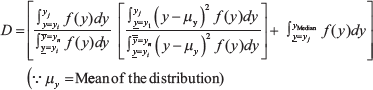
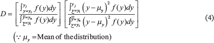
Where, the degree (D) would vary from zero to one. i.e. 0 ≤ D ≤ 1.
Equation (4) uses the concept of an index of trade concentration of the form

where σ2 A = variance of the area A and σ2 A + B = variance of the total area A + B and A + B = 1. The variance ratio considers the variations of the production and the supply of output at different times.
When the change in the equilibrium bid or wholesale price ∇xi = y is zero, then competition is there, and the degree of the cartel is zero. Here xi is not stationary.
When a change in the equilibrium bid or wholesale price ∇xi = y is positive, and the pdf f(y) exists, then competition is not there, and the degree of the cartel is non-zero.
When a change in the equilibrium bid or wholesale price ∇xi = y is positive, and the pdf f(y) exists then competition is not there, and the degree of the cartel is one if area A = 1, so that A + B = 1 and
The most critical questions are one, reasons for concentration in area A, and how to identify these highly probable areas?
The range of area A is
Lemmas 1 and 2 explain that the change of equilibrium bid price follows the power law. To measure the degree of the cartel, it is required to identify the area under f (y). The degree of the cartel is the area until is reached from the highly frequent point of y on f (y) (Lemma 3).
Empirical Measurement
The measure of the degree of cartel here is period-centric. If you are interested in measuring the degree of the cartel for any given period, then the present model is appropriate. We are interested in further considering the dynamic nature of variables, such as the demand cycle. Our model is essential because agricultural production is seasonal and, in the price, behaviour is full of seasonal effects. Hence, for example, if any farmer wants to sell his/her produce in the current period for the product, then the information on the degree of the cartel for the last period would help choose the correct market. Moreover, if the market-wise information on the degree of the cartel is available in the public domain, the competition in between the markets would also increase. Considering the above points, we have incorporated de-seasonal effects in the model to generate an accurate degree measure for any given season.
To measure the degree of the cartel, the following steps are required:
Identify the period for which the degree is to be measured and collect the wholesale price for a given market. This could be weekly, monthly or daily. Exclude the seasonal effects. Test of stationarity of the original data and the difference. If stationary, then derive the first difference in the data taking all the change as positive. If a negative value finds, then consider it as positive. If it is not stationary, the process stops here, and the method does not match the situation.
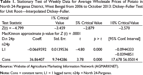
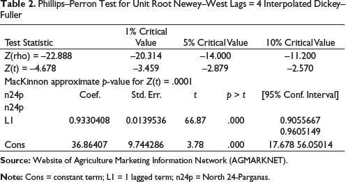
Dickey–Fuller (DF) test (Dickey & Fuller, 1979) and Phillips–Perron (PP) test (Phillips & Perron, 1988) are used for unit root to test stationary in time series data. The DF test take care of possible serial correlation in the error terms by adding the lagged difference terms of the regressand. Phillips and Perron use nonparametric statistical methods to take care of the serial correlation in the error terms without adding different terms. Therefore, to test stationary in time series data, if the DF test model becomes insignificant, then PP test for unit root will be appropriate. DF and PP tests help control the seasonal effects and translate the data in joint distribution for any given period for which the degree of the cartel will be measured. The DF and PP tests are the required calculation, and after this measure, the degree will be calculated.
Derive the empirical probability distribution function. If the area exists, then using the above formula calculates the degree of the cartel.
If the cartel is there, then the original data and first difference would be stationary because the same set of traders are bidding the auction sequentially. If the original data difference is non-stationary, but the first difference is stationary, then there is a high chance of cartel with a low degree because the set of bidders are changing over time. Agricultural commodities are perishable and seasonal effects are also there. De-seasonalization would be helpful to check these problems of seasonal effects.
Case 1
In the first case, we measure the degree of the cartel in the rural wholesale market in the presence of large traders with quality preference. Das (2019a); Das (2019b) shows that in the presence of large traders (heterogeneous demand) in the rural wholesale market, small and large traders form an informal relationship and a cartel among them. He derives the wholesale price per unit that acts as a benchmark during the auction process as the MSP based on the market interaction using symmetric retailers (both large and small) by
Stationary Test of Weekly Data for Average Wholesale Prices of Potato in North 24-Parganas District, West Bengal from 2006 to October 2013: Dickey–Fuller Test for Unit Root—Interpolated Dickey–Fuller.
Phillips–Perron Test for Unit Root Newey–West Lags = 4 Interpolated Dickey–Fuller
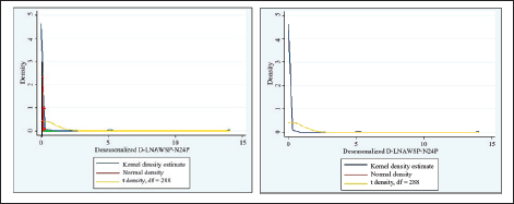
From Figure 2A From the above figure 2A it is seen that the B area is zero. Therefore, the Degree of cartel = D = 1. Here the price fluctuation is close to zero. This has been explained theoretically below:

Here D = 1, as the area A = 1 and B = 0. Moreover, the variance of B = 0 (from Figures 2A and 2B). Here the slope is steeper. Higher is the steepness, more would be the degree of the cartel. This degree is supported by the findings in (Das, 2019b). It has been shown that the traders control the market in the North 24-Parganas in the presence of large traders. This study explains that the fixed costs in the grading of the quality products created the market imperfect. This has been reflected in the APMC market as well. The theory has been explained in the paper by Das (2019b). In the paper, Das derives the power law. In this paper, the formal degree of collusion has been measured on the same distribution and shown that the degree of the cartel is one. This means the market is controlled by the bidders/traders completely.
Case 2
Stationary Test of Daily Wholesale Price of Onion of Nashik District for the Market Lasalgaon from the Year 2006 to 2019 after De-Seasonalization on Absolute Difference of the Original Data.

Phillips -Perron Test for Unit Root Newey -West Lags = 4 Interpolated Dickey - Fuller.

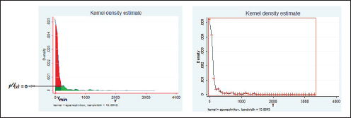
From Figure 3, it is seen that the B (green) area is not zero. Therefore, the degree of the cartel is D < 1. Here degree is close to one as area A is close to one and the B ≠ 0. Moreover, the variance of A and B is non-zero. Here the slope is steeper. Higher is the steepness, more would be the degree of the cartel. Therefore, using the formula, the actual degree of the cartel is D = 1, considering all the densities whose values are present after three zeros after the decimal point, that is, three zeros placed before other digits. The consideration of the densities where three zeros are placed before other digits is in the red area. Any density with more than three zeros placed before other digits is under the green area. Calculation of area considering the values beyond three zeros would make it difficult to calculate. The four zeros before any other digits points start from the point where
Conclusions and Limitations
This paper derives a standard theoretical measurement method to measure the collusion among the bidders in an open ascending price auction. Identification of cartel in any open ascending price auction would be possible considering the repetitive behaviour of the auction at different times. This research derives a standard method of measuring collusion using the dynamic data and the behaviour of the equilibrium prices at different times. This paper also measures the degree of collusion in two important agricultural commodity auction markets. Using the existing publicly available data for two agricultural commodities, namely potato and onion, the results show collusion among traders in agricultural commodities markets, and the markets are controlled by the bidders/traders completely.
This research helps and improves future research in the reforms in Indian agriculture and other countries where the conditions of this type of market exist. Identification and knowing the policy implication in the agricultural market reforms would be easier to understand, and remedial measure can be taken accordingly. The findings would help to study the link between the supply of the commodity and the degree of collusion. Identifying different small cartel groups at different times with respect to the supply of the agriculture commodity would help avoid the incidence of distress selling by farmers, which is the main hindrance in the development of the farming community in India.
The agriculture market is different from other markets, say, manufacturing (e.g., automobile) or service (e.g., transport) where cartelization is present. This is why we have considered agriculture only in this study. However, we are planning to work on other markets in future.
This study is based on the buyer, seller and auctioneers for a given product on the auction floor. The externality has been incorporated into the behaviour of three agents. For example, if inflation is there, then the disagreement point or the MSP will be charged accordingly by the auctioneer. On the other hand, buyer and seller will also consider the other market behaviour in their bidding process. For example, if the input prices increase, this will affect the bid price as the seller would not accept the bid value if it does not cover the increased input prices. Therefore, the present model considered externality indirectly.
Moreover, no such measure is there to quantify the degree of the cartel in the auction markets. This paper will be a pioneer in the field. In future, the model will be developed further considering the changes in the policies and the market conditions.
Appendix
Appendix A
Let us assume there is a finite set of bidders n. The above theory says that the highly valued bidders always participate in the bidding process. If bidders are in ascending order, say (1,2,3,…k,…,n) then if k number of bidders form a cartel and win the bid in every sequential auction. As a result low valued bidders, that is, (n – k) set of bidders will be losing the auction. Therefore, the value will not be recorded and the winning bid price by the k number of bidders will be the equilibrium bid price. Therefore, the change of the equilibrium bid price starts with the smallest positive value due to bid by the cartel. If we consider a fuzzy variable µ woth the variable y, the change of the equilibrium bid price then there would be a horizontal variation in the highly frequent value of y, that is, (y ± µ). Therefore, The f (y i ) starts from the highily frequent point and y i = y I .
For example, when (n – 1) numbers of bidders are in cartel then the lowest valued bidder 1 will be crowed out from the market to being included in the cartel. Hence if competition increases with the increase of the number of bidders then the value of f (y i ) corresponding to the new out of cartel equilibrium bid price will decrease as that bidder is not in the cartel and not regular like the cartel bidders. Therefore, if cartel exists then there is a negative relationship between the f (y i ) and the number of the new bidders who are not in the cartel. A sequence a0, a1, a2,…,a n of real numbers is called unimodal if the sequence increases steadily at first and then decreases steadily (Heim & Neuhauser, 2019; Wilf, 2006). Then the following lemma is also true.

This is a sequence of the value of the individual bidder.
The first difference of the sequence is

This is a sequence of the difference between the value of the individual bidder.
The sequence (i) is log-concave if a2 ≥ a+1a–1. Here as a–1 = 0. Therefore, the sequence is log-concave. Therefore, cartel happens among (k – j) members where the leader is valued at a then the cartel will win the bid and their objective function; difference sequence b1,b2,…b–1 has no value as they are not in the cartel and they will not win. Therefore, the unimodal point is at a and the objective function will be maximum at (|a – a| = b). For the sequence b1,b2,…b–1 the mode is b–1 because b–12 ≥ b–2 b.
Shifting the scale, we get b2 ≥ b – 1 b + 1. As b – 1 does not exist in the objective function so, b – 1 = 0. It concludes that the sequence starts from b as it has the highest mode in the sequence b, b + 1,b + 2,…,b + i .
If a new bidder without information enters into the bidding process, then that bidder would start to win the bid and bid at a price above the highly frequent bid price. In the absence of the new bidder after the highly frequent point, the pdf is
Let the sequence of the equilibrium bid is a0, a1, a2,…,a –1,a
The first difference of the sequence is
Here kth bidder would win the bid as all k bidders in cartel attain equilibrium price a0.
Here the new bidder will bid more than a0, sequentially and the bid process would stop following a sequence a0 < a1 < a2 <… < a. Therefore, say if new bidder i enters between a0 and a1, as a0 < a < a1 then | a0 – a| > | a0 – a1|b0+1. Because when all k bidders are in cartel then a0 = a1 = a2 = … = a – 1 = a. Therefore, the rate of fall, that is,
The area of concentration starts from the lowest possible change in bid price or the point of y = y for which f (y = y) is maximum. The area of concentration ends at the higher possible change in bid price or the point of y
i
for which
Appendix B
There are three types of prices available for each day of the auction. These are minimum, maximum and modal prices. The above formula is based on modal prices. But if we consider this fuzziness of equilibrium price then the degree of measure has to incorporate this fuzziness. The degree measure derived above is

To incorporate the degree of fuzziness the variable y must be redefined. As y is the change of the original equilibrium variable, so let the original bid price be x. First adjust the fuzziness to x and then derive the variable y. The adjusted variable x is
where
X = Fixed or crisp value of the equilibrium bid price here Min value.
Where θ = (1 – α),
Where λ = (1 – α), λ = (1 – α),
Now derive yF using the new variable 
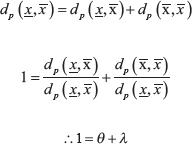
A suitable measure of fuzziness is to be used to calculate θ and λ. Let X be a nonempty set. A real-valued function d on X × X is a metric where 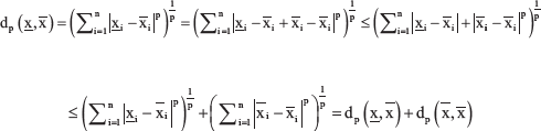
Or,
Footnotes
Declaration of Conflicting Interests
The authors declared no potential conflicts of interest with respect to the research, authorship and/or publication of this article.
Funding
The authors received no financial support for the research, authorship and/or publication of this article.
