Marriage,Quarrels,and Lovemaking

Introduction

Statistical predictions made by combining a few ratings and following a rule can sometimes outperform the subjective clinical predictions of trained professionals (Meehl, 1954). Intriguingly, ‘improper’ rules that combine predictors with equal weights can be just as accurate in predicting new cases as ‘proper’ rules, such as those from regression analysis (Dawes, 1979; Kahneman, 2011). A possible explanation is that improper rules are not affected by accidents of sampling (Dana & Dawes, 2004). For example, one improper rule is that we can predict marital stability by the frequency of lovemaking minus the frequency of quarrels (Dawes, 1979).

From 30 self-described happily married couples in a study, only two argued more often than they had intercourse, while 12 self-described unhappy couples argued more often (Howard & Dawes, 1976). Furthermore, when partners rated happiness from ‘very unhappy’ to ‘very happy’, the correlation of the rate of lovemaking minus the rate of quarrels with these ratings of marital happiness was 0.40 (p < 0.05) (Dawes, 1979). These findings were replicated afterward (Edwards & Edwards, 1977). Moreover, when partners monitored their lovemaking and quarrels after the ratings of marital happiness, the correlation between the sex–quarrel difference became higher (0.81, p < 0.01) (Thornton, 1977).

Dawes (1979) concedes this ‘is not very profound, psychologically or statistically. However, the point is that this very crude, improper linear model predicts a critical variable: judgments about marital happiness’.

Here, we revisit this classic literature to provide the missing theory for the improper rule of marital stability. In addition, we put forward a model in line with Becker’s (1981) family economics and provide initial survey evidence for our model assumptions.

Model

The conflict between the sexes reflects different sexual strategies, not competition for resources. Both sexes have short-term and long-term mating strategies, and marriage may result from a long-term strategy. Humans are a species with internal female fertilization. One act of sexual intercourse can produce a 9-month pregnancy and 4 years of lactation for a female. This fact renders females more selective than males about mating. Females manifest interest in males who provide the resources to bear their heavy reproductive investment, and males are interested in providing the resources valued by females to have sexual access to them (Buss, 2019). This picture suggests the hypotheses of our model.

The mating market is not perfectly competitive because the choosy female has some monopoly power. Moreover, while sex and resources are essential complements in reproduction, their preference orderings differ for males and females. Resources are more valued than sex for females, while the reverse is true of males. Moreover, while resources are a private good, sex is a public good that is consumed jointly. Furthermore, while both sex and resources are critical for males and females, we consider sex is a good for males and a bad for females. This modelling convenience allows us to share the model of smoke and money in an externality analysis using Edgeworth box.

We set sex and resources as perfect complements and thus assume Leontief preferences:

U m = min ( 2 S , M )

(1)

and

U f = min ( S , 2 M ) ,

(2)

where U _m and U _f are the utilities of husband and wife respectively, S is sex and M is total couple money. Resources are represented by money because they can be considered a composite good with a price equals to 1. Husband values sex over money in a 2:1 ratio (Equation (1)); and wife values resources over sex in a 2:1 ratio (Equation (2)). Though total couple money enters the utility function of each, what is held privately is a fraction of M, and thus resources distribution matters.

Figure 1 displays square Edgeworth boxes representing these preferences. The lines show indifference maps of infinite L-shaped Leontief utility functions. Because of the chosen ratios of 2:1, the indifference maps reduce to indifference lines for husband (blue) and wife (red). The left box shows two (top and bottom) corner equilibria. On top of that, the husband has unconstrained access to sex and the same resources as the wife. From the wife’s point of view, there is too much sex and too few resources for her. This situation is likely to be an unstable equilibrium because quarrels started by her can overshoot the frequency of sex. At the bottom, equilibrium is likely to be unstable, too. The husband ignites quarrels in the face of a null frequency of sex. Remember, the conflict between the sexes is a result of different sexual strategies. For this reason, here we assume quarrels start because of the mismatch of the quantities of the desired sex.

OPEN IN VIEWER

Figure 1.

Source: The authors.

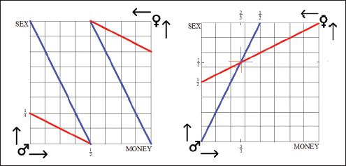
We can prevent these two unstable extreme equilibria from occurring by removing the endowments of resources of the husband and wife, as on the right-hand side of Figure 1. This pure exchange marriage with no external parties (auctioneer) setting prices reaches an equilibrium with less sex than husband desires and the resources distribution favouring the wife. Sex is only two-thirds of the unrationed frequency, and the wife gets two-thirds of the total couple’s money. Thus, in equilibrium, 0 < S <1. Given the circumstances, this is an allocation that pleases both the husband and wife. However, because of the wife’s monopoly power in the supply of sex, the husband ends up with relatively fewer resources. Thus, the husband has to ‘pay’ for sex.

The indifference lines suggest an equilibrium, even though Leontief utilities, in general, are not strictly convex and thus do not satisfy Arrow–Debreu requirements for the existence of equilibrium.

In Figure 1, the exchange takes place through a process of personal bargaining. Thus, we do not consider relative prices and a budget line. However, equilibrium is possible even when we introduce the relative prices of sex in terms of resources for husband p ^m _s and wife p ^f _s . Adapting Lindahl equilibrium in a smoky box (Bergstrom, 2020), the frequency of sex S maximizes (p ^m _s + p ^f _s )S over all possible values of S. Because 0 < S <1, this is possible only if p ^m _s + p ^f _s = 0. Therefore, p ^m _s = − p ^f _s is Lindahl equilibrium.

Lindahl budget constraint for the husband is p ^m _s S + M _m ≤ W _m , and for the wife is p ^f _s S + M _f ≤ W _f , where total goods allocation is W = W _m + W _f . Remember the composite good price is 1, but money is now explicitly split between husband and wife, M _m and M _f .

After considering Lindahl equilibrium and the above budget constraints, the wife’s budget constraint in equilibrium is p ^m _s S + M _m ≥ W _m . Comparing this result with the husband’s budget constraint, there is at least one point where their choices coincide.

To see how the wife’s Lindahl budget constraint becomes p ^m _s S + M _m ≥ W _m in equilibrium, first note that the wife’s consumption of the composite good M is the consumption of the total goods W minus the husband’s consumption of the composite good M _m (see a similar formalism in Bergstrom, 2020). Thus, we can rewrite the wife’s budget constraint as p ^f _s S + (W − M _m ) ≤ W − W _m , which simplifies to M _m − P ^f _s S ≥ W _m . Then, after substituting Lindahl equilibrium p ^m _s = − p ^f _s into the latter equation, we get the wife’s budget constraint in equilibrium p ^m _s S + M _m ≥ W _m , which is written in terms of that of the husband. (See an analogous derivation in the Equations 5.1−5.3 of Bergstrom, 2020.)

For more general preferences U ⁱ = (S,M) (Aizer, 2010), assume that M _m + M _f ≤ M, that U ⁱ _s (0, M) > 0, that U ⁱ _ss (S, M) < 0, and that for some large enough S, U ⁱ _s (S, M) ≤ 0 (saturation). This setup is sufficient to generate a contract curve in the Edgeworth box, where U ^m _s (S, M) > 0 and U ^f _s (S, M) < 0 at the point of equilibrium. So, if the two spouses have resource endowments, then at the equilibrium, the husband pays for sex by giving up resources—that they both enjoy—to get more sex—that he enjoys, but the wife does not.

The takeaway message is, the source of quarrels in marriage is the mismatch between a given allocation of sex and resources and the evolutionarily set preferences of husband and wife.

Data

We gather further evidence for the marital stability formula and initial evidence for our model assumptions by resorting to previous literature and a light-hearted questionnaire.

In a survey (Meston & Buss, 2009), 1,006 women report as many as 237 reasons for having sex, suggesting no specific reason for a woman to have sex. So, it is not that far-fetched that a female views sex as a bad.

Marital stability does not equate to marital happiness. Evolution shaped human bodies and brains not for happiness but to maximize reproduction (Nesse, 2019). The evolutionarily set preferences of males and females are suitable for their genes but not for them. For example, sex is consumed jointly but inevitably out of sync because of the location of the clitoris. This circumstance is a source of female monopoly power in the supply of intercourse because a woman does not need to orgasm to reproduce.

Given their preferences, it is puzzling that males seek marriage, but this comes from a ground-rule set by females: obtain long-term male commitment before consenting to sex. However, there are adaptive benefits that accrue for a married male, including increased odds of attracting other females, especially the most desirable ones, increased paternity certainty, greater survival and success of children benefited from his investment, higher social status, more coalitional allies, access to the wife’s resources and status and increased lifespan (Buss, 2019).

As for the survey evidence, we asked Brazilian heterosexual married couples from our contacts the following questions. Because the assembled sample excludes divorced couples, we thought it needless to ask if someone was ‘happy’.

Questionnaire

If you are married and heterosexual, please answer the questions below:

Were you born male or female?

From 111 responses (wives, 70%; husbands, 30%), most husbands and wives of almost all ages agreed that the husband in their relationship spends more. However, for the age range 25–34 years, the husbands and wives agreed the wife spends more. We can explain the latter result by the opportunity cost of being married given by the mating market value of men and women. Mate value is one’s overall desirability to members of the opposite sex. The mating market value of a woman peaks at 20, and that of men is highest at ages 25–30 (Buss, 2019). So, the opportunity cost for wives is highest in the age range 25–34.

There was an intriguing convergence of reports of low sexual intercourse and few quarrels for all ages, even considering these are Brazilian couples. Moreover, both husbands and wives reported little refusal of sex from the wife, and wives were more emphatic in their reports.

Of note, it is the ‘remembering self’ that responds to questionnaires, and so responses are expected to be biased by memory (Campara et al., 2021). Ideally, one should give a voice to the ‘experiencing self’. However, we think this problem does not arise in the critical Question 6. Because of its comparative format, participants are likely to make ‘System 2 judgments’ and not based on memory (Campara et al., 2021).

Most wives reported more sex than fights in all ages, apart again from the age range 25–34. Remember, this is the age range where wives are perceived to spend more than husbands, and so the fights are possibly just enforcing the wife’s monopoly power in the supply of intercourse. Husbands of all ages reported more sex than fights, too, but these statements are suspect. Men tend to overreport their number of sexual partners (Buss, 2019), and thus we expect them to report more sexual intercourse with their wives. Therefore, the responses from husbands and wives suggest that the formula of marital stability is more likely to apply to couples with the highest mating market value. The data set is available at https://doi.org/10.6084/m9.figshare.13681729.v1.

Conclusion

The frequency of lovemaking minus the frequency of quarrels is claimed to predict marital stability. Here, we provide the family economics of this ‘improper’ rule by resorting to insights from evolutionary psychology. We also present survey evidence. Evolution predetermines females to value resources more than sex, and the inverse is true for males. While resources are a private good, sex is consumed jointly. However, sex and resources are perfect complements that Leontief preferences can model. A pure exchange marriage reaches an equilibrium with less sex than the husband’s desire and distribution of resources favouring the wife. This result is a consequence of the wife’s monopoly power in the supply of intercourse. Equilibrium is also possible when we introduce prices into the model. It is then implied that quarrels in marriage result from the mismatch between a given allocation of sex and resources and the evolutionarily set preferences of the husband and wife.