




Abstract
This article studies the relation between class and electoral participation. While the relation between political participation and many demographic variables such as caste, gender, age and location has been well researched in India, the same is not the case for the relation between class and electoral participation. Multiple measures of class (income, asset-wealth, occupation and education) are explored and conceptualized in this article, following which these measures of class are operationalized using the National Election Study datasets covering a twenty-three-year period (1996–2019). Each of these measures is used to trace the relation of class with two outcomes of electoral participation (turnout and party vote share) over time. Disaggregation by gender, locality and caste is provided. Finally, regression analysis to study the impact of these variables on turnout and vote share reveals the complexity of class. We find a complex picture of turnout and party choice with variation across different class measures. More significantly, variations in results raise questions about the usefulness of existing class indices. Further, we find that the type of measure being used affects different outcomes differently. For turnout, income and wealth seem to be better predictors, and for party vote share, subjective class is a better fit, whereas asset-wealth displays opposite patterns to income and subjective class in some instances.
Introduction
Election research, including the analysis of patterns of electoral participation, has had a fairly established history in the Indian context, with the use of Election Commission data and the National Election Studies (NES) datasets providing a benchmark for rigorous national-level comparative research (Kothari, 1973; Kumar, 2009; Yadav & Palshikar, 2008). 2 Much research has focused on the patterns of political participation by different groups and communities. In particular, patterns of voting by gender (Deshpande, 2009), caste, tribe and religion (Alam, 2009; Kothari, 1973; Vaid, 2009; Yadav, 2000) have been studied. Theses have been proposed on the resurgence of political participation in India at the margins, or the ‘second democratic upsurge’ (Yadav, 2000), along with critiques of this argument (Palshikar & Kumar, 2004). In all of this, the focus on class has been limited (see the following section for a discussion of the exceptions; see Fernandes and Heller [2006] on the middle class, and also Sheth [1999], and Ahuja and Chhibber [2012]).
A possible reason for fewer studies on class in India is its secondary position to caste in the academic discussion and sometimes a conflation with it (Vaid, 2018). Another reason could be issues around the measurement of class. While variables such as caste may have their complexities, there are direct ways in which surveys have captured them. For class, however, there are a variety of definitions and measures that may preclude a truly comprehensive or comparative study over time.
Given the range of definitions and measures of class, this article has a twofold aim. The first is to compare and contrast available indicators of class and their relation to two components of electoral participation: turnout and party vote share. 3 The second aim is to analyse the relative impact of these measures on turnout and vote share. Together, this allows us to study the concept of class, its operationalisation and its impact on electoral participation, and whether there is any evidence of class-based voting in India.
This article uses the NES post-poll data for elections held between 1996 and 2019. Since there has been variation in the measures of class used to study political engagement, this article provides a comparison across four ‘objective’ measures of class used previously as part of class indices: asset-wealth, income, occupation and education. To this we add a discussion of ‘subjective class’, or class self-identification. Using these disaggregated measures of class rather than one combined index allows for a comprehensive comparison of key patterns of electoral participation over the years. Further, studying the impact of each of these measures of class on turnout and party choice in the 2019 general election helps focus on the comparisons across measures of class for one year in detail.
We find a complex picture of turnout and party choice with variation across different class measures. More significantly the variations in results raise questions about the usefulness of existing class indexes. Further, we find that the type of measure being used affects different outcomes differently. For turnout, income and wealth seem to be better predictors, and for party vote share, subjective class is a better fit, while asset-wealth displays opposite patterns to income and subjective class in some instances.
The following section of the article discusses the key literature on class and macro-patterns of electoral participation, followed by a discussion on data and measures used; this is followed by a section on turnout and vote-share patterns by objective and subjective classes; the article then compares these patterns by caste/community and class measures; the penultimate section compares the relative significance of various measures of class on electoral outcomes, and the last section concludes.
Literature Review
A review of the literature highlights the ways in which class is conceptualised and operationalised in electoral research and the variation in the findings. Kumar (2009) using the NES data had commented on the ‘slight increase in turnout among middle class voters’ following the 2009 Lok Sabha elections and concluded that ‘this was a classic instance of the democratic upsurge levelling off’ (p. 50). For his study, he used the NES classification of economic class: upper, middle and lower. His classification codes information on monthly household income and household assets (Lokniti Team, 2009).
For the 2014 NES data, Sridharan (2014) used a ‘composite class index consisting of a combination of economic (income and ownership of selected durable assets, in particular the type of house) and sociological criteria (that is, occupation and occupational level), with assets and income adjusted for rural and urban locations …’ (p. 72). This classification divides the sample into upper middle, middle, lower and poor classes. Further, using the 2019 NES data, Sridharan (2020) used the NES class index of ‘income, house type, occupations and occupation level’ (p. 52). The details of the index, whether it uses weights, or is simply additive, or what the ‘occupation level’ implies are not provided. The author finds that the measures of class are ‘not comparable’ (p. 52) across 2014 and 2019. Using the NES class scheme, he divides the sample into poor, lower, middle and rich and looks at turnout, party choice and a range of political opinion variables age-wise, by rural–urban location and by caste. He finds that ‘the degree of class polarisation in party preferences seems muted’ (p. 58), though he finds a pro-BJP swing among the lower classes (across groups with the exception of the Muslims).
Jaffrelot (2015) using the NES data provides more detail for 2014. He shows that the NES class variable is a combination of ‘occupation, type of housing, selected household assets and income’ (p. 34), providing details of each of these, including an index comprising housing type, occupation and assets and an income index. His classification also divides the sample into poor, lower, middle and rich. Jeffrelot comments on the change in the ‘reverse correlation between the socio-economic status and electoral participation’ with an increase in the participation of the middle and upper-middle classes in 2014 (p. 20). He finds that ‘class has become a more influential factor and has significantly contributed to Modi’s success’ (p. 34).
As we see, different measures of class using the same database have been used across the years. While these measures have been described by the authors as an ‘objective class index’, the technical classification seems to be based on ‘predetermined criteria’ (Jaffrelot, 2015, p. 34) that might involve some subjective decisions. For example, why place a particular occupation in one class and not another (since occupation is difficult to code hierarchically unlike income, for instance)? Further, conflating measures that comprise household-level information (income and assets) with individual-level information (occupation) seems conceptually and empirically problematic, especially since household resources are seldom equally distributed within the family (Vaid, 2018). How would we then discuss women’s political participation in this context? These questions particularly underline the confusions caused due to inadequate engagement with conceptualising class, prior to operationalising it (Vaid, 2018). What precisely is one measuring is an important question that needs addressing.
Further, the use of varying definitions of what comprises class, along with differing asset information across the years (discussed later), as well as a fairly subjective understanding of who is considered poor, middle or upper in terms of income, creates the additional problem of ‘class’ not being comparative over time. Looking at individual variables that comprise class separately might allow for some more consistent over-time comparisons.
While this article provides a small step forward towards establishing patterns of electoral participation in India by including class in its various complexities, there are limitations of such a study. In addition to the inconsistencies in the data on measures of class, the following questions arise: Which of these measures is most appropriate in capturing the differences in whether people decide to vote or not, to choose a particular party, or to participate in activities around the time of elections? Some of these questions have been studied by researchers (e.g., for Britain, see Andersen and Heath [2002]), while others have looked at whether class mobility makes a difference to voting (de Graaf et al., 1995; Nieuwbeerta et al., 2000). Other questions also arise: which measure best captures class location and class identity? Or do they all tap different dimensions of this identity? Should we move towards constructing a comprehensive measure of class? What would be the basis to make this categorisation consistent over time? Or is class by definition difficult to capture and hence any measure, if adequately discussed, can be used based on the purpose of the study? While all these questions cannot be answered here, the discussion in this article opens up possibilities for future research in this area.
Data and Concepts
This article uses post-poll NES data from 1996 to 2019 from the Centre for the Study of Developing Societies (CSDS). This includes surveys covering the Lok Sabha elections of 1996, 2004, 2009, 2014 and 2019 (see Figure 1 for sample sizes). The two elections of 1998 and 1999 are excluded from the present analysis because of two reasons. First, the sampling strategy was different for the 1998 and 1999 surveys when compared with those of the other years. NES 1998 and 1999 were part of a panel design in which the 1996 sample was used as a base, and additional respondents were added owing to attrition (see Lokniti Team, 2004). In order to keep parity between the years, we have selected the first of the panel years (1996) for our analysis. Second, the 1998 survey also has limited use given the purpose of the present article because questions on asset ownership and income were absent in that survey (a question on income is absent from 1999 as well).
The NES surveys used in this article are individual-level post-poll surveys with data collected through the use of stratified random samples from the electoral rolls in the period between polling and declaration of results. Except the 1996 data, the other datasets were collected at the state level and then aggregated to the national level. Because of this, and to avoid concern about inflation in turnout owing to the social desirability bias (Holbrook & Krusnick, 2010), this article uses data-specific weights provided by CSDS to account for actual turnout and party choice. 4
We turn to the operationalisation of the key concepts used in this article.
Class
Social class is a contested concept theoretically and empirically (Kumar et al., 2002). While there are disagreements regarding the conceptualisation of class (Giddens, 1980), there are some agreements on ways of operationalising it (though each school arrives at these operationalisations from varying theoretical paradigms). The key operationalisation in sociology is often occupation (both in terms of relation to ‘means of production’, closer to the Marxist conceptualisation, and relation to the ‘market’, a Weberian conception; see Wright [2006] for a discussion). Economists, however, have used wealth and income to measure class. Furthermore, education is seen to measure ‘social’ class or status, especially if seen through the lens of ‘capital’ (Bourdieu, 1986). 5 Much of the previous research using NES’s own measure of ‘class’ has conflated several variables, where specifics of the definition of class, or its measures or weights ascribed to assets etc. has not been consistent or explicated clearly over time. This section briefly discusses how each of these concepts is operationalised in the present study.
As mentioned, this article uses four measures of class: asset-wealth, income, occupation and education, and for 2019, a ‘subjective’ self-identification measure that has not been extensively studied with regard to class-based patterns of voting is used (see Kapur et al. [2018] for the implications of increasing middle-class self-identification on politics).
In the NES, the income data collected at the household level were converted into income quintiles. There is no information on income in 1996. In 2009 and 2014, household income data were collected on a continuous scale. For 2004, data were collected in 8 grouped categories, and in 2019, they were collected in 11 grouped categories. 9 Owing to variations in how income was collected, the conversion into income quintiles is not without its problems, especially for the two years (2004 and 2019) in which grouped ordinal data are collected. However, the closest approximation to quintiles is calculated using percentiles (see Tables A2 and A3).
Table A7 includes the descriptive frequencies for these measures of class across the years. Regarding correlations between the various measures (see the heatmap in Table 1), the strongest overall correlation is between income and asset-wealth (r = .545) and between education and asset-wealth (r = .458); both these correlations are moderate in strength. Occupation has the weakest correlation with all the other variables (which is not surprising since occupation is not strictly ordinal and also reiterates the discomfort with including occupation in a class index with the other variables such as income/assets). Further, there is a weak to moderate positive correlation between the self-identified class and wealth (r = .395), followed by the self-identified class with income (r = .292) and with education (r = .276). The weakest correlation of subjective class is with occupation (r = .098). This brings out the complexity of the conceptualisation and operationalisation of class. The operationalisation depends on the purpose of the study. If the hypothesis (as discussed by previous authors) is of the increase in the middle-class vote and its significance for the BJP-led National Democratic Alliance (NDA), 13 then which measure of class would be more appropriate as the correlation between subjective class and other measures is weak or moderate? Although this article does not answer this question, by disaggregating various components of class, we capture a more comprehensive picture of class-based participation.
Correlation Heatmap, NES 2019.

Electoral Participation
Political participation is a broad concept that comprises electoral participation and participation in political activities outside the election period. This article focuses on two outcomes constituting electoral participation: first, the act of voting in an election (henceforth referred to as ‘turnout’) and second, the choice of political party (party choice). Studying broader political participation as captured by the respondent’s participation in election-related activities such as canvassing, etc. and political interest is important but outside the scope of the present article. However, we use an index of election-related activity or ‘political participation’ and ‘political interest’ as control variables in the regression analysis, to study whether they impact turnout and party choice. 14
Patterns of Electoral Participation by Class
This section analyses the relation between various measures of class and turnout and vote share. The disaggregation of electoral participation is provided by gender and locality (using rural and urban as broad categories to maintain consistency across the years). As class is closely tied to caste, while caste/community 15 are not a central focus of this study, the interaction between community, class and electoral participation is discussed later.
Turnout
Figure 1 graphically displays the turnout between 1996 and 2019. The first set of bars represent the overall turnout figures across the years, the second set disaggregate these figures by asset-wealth, the third by income quintiles (this excludes NES 1996 that did not collect this information), the fourth set by the occupation level and the final set by education. This section summarises the broad patterns in the data, the implications of which are explored in the concluding section.
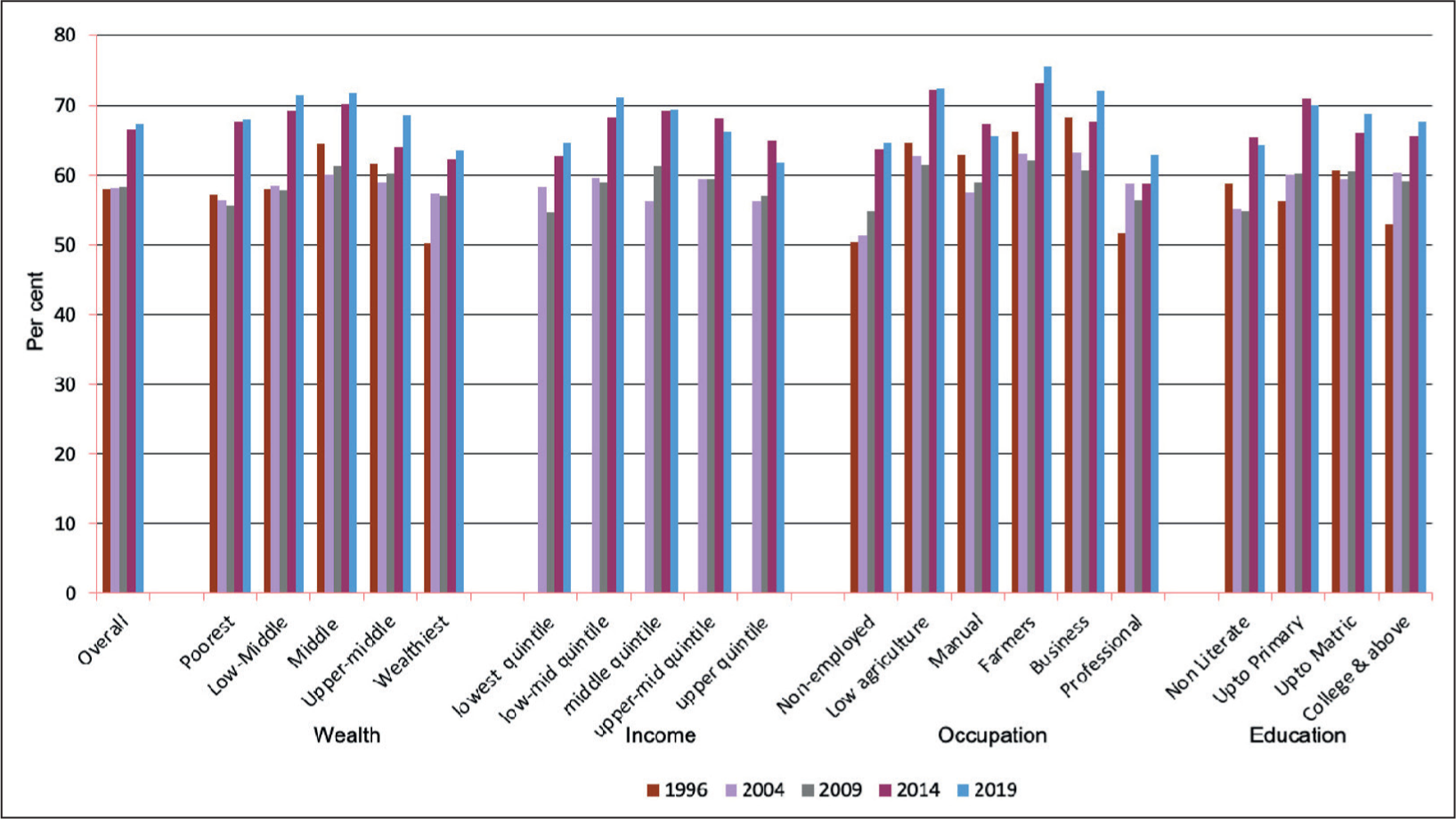
Although turnout was consistent around the 58% level between 1996 and 2009; 2014 and 2019 stand out with substantially high turnout. However, there is no distinctive pattern of a smooth increase or decrease in turnout by measures of class.
Asset-wealth-wise turnout figures indicate a slight inverted u-shaped curve, with those in the middle quintiles turning out more than the two extremes in all election years. In the last two general elections, it is the asset-poorest (and the lower-middle) who are turning out to vote more than those in the upper-middle and wealthy categories.
A similar inverted u-shaped pattern is seen in terms of income quintiles. The middle-income quintile in all years except 2004 (where the skew is towards the lower quintiles) has the highest turnout with some distinctions across the years. For 2009–2014, the pattern is an exact inverted u-shape, and for 2019, while an inverted u-shape is maintained, the peak turnout is for the lower-middle rather than the middle-income quintile. Also, over 2004–2014, there has been an increase in turnout in each subsequent election for those in middle, upper-middle and upper-income levels.
For education, in most years, the highest turnout is for those with education up to the primary (2004–2019) or up to the matriculate level (1996), which are the two middle education categories in the data, thus displaying another rough inverted u-shaped curve. Except for 1996, the lowest turnout for all years is for the non-literate.
Occupation is an exception. This is not surprising given that occupation is not an ordinal variable unlike the other variables discussed. The occupation patterns show us the distinction between the pre- and the post-2014 elections. Before 2014, turnout in order from highest was business, farm, lower agriculture, manual and professionals, with the lowest turnout for the homemakers/non-employed. Since 2014, it is the two farm categories, followed by business, manual, the non-employed/homemakers and finally the professionals with the lowest turnout.
In order to capture whether there are gender or rural–urban differences in turnout, we study the odds ratios of turnout. These odds ratios are a measure of the odds of a woman (or someone in an urban area for the locality-wise ratios) voting, compared with the odds of a man (or someone in a rural area) voting. An odds ratio of 1 implies that gender (or locality) and turnout are ‘independent’ of each other (Yadav, 2000), and hence there is no gender or rural–urban difference in turnout. An odds ratio less than 1 implies that women (or people in urban areas) are less likely to turnout than men (or people in rural areas), and conversely, an odds ratio greater than 1 implies that women (or urban) are more likely to turnout than men (or rural).
We find (Table 2) that the odds ratio of women turning out to vote compared with men has been increasing over the election years (with a slight dip in 2004). In 1996, for every 100 men who turned out to vote, 84 women voted, while in 2019, for every 100 men who voted, 95 women voted.
Odds Ratios of Turnout by Gender and Locality 1996–2019.
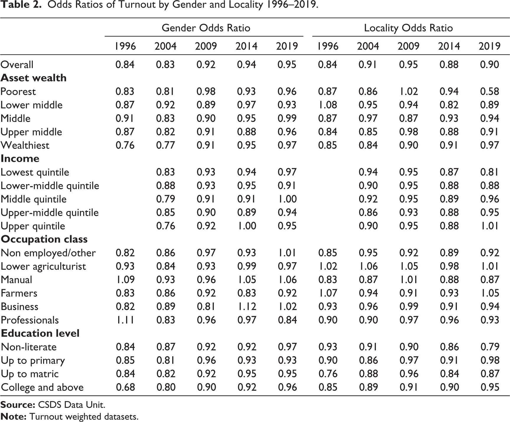
There is no clear pattern across years by asset-wealth. In 2019, the gender odds ratios are close to 1 for the middle class, and quite high for all classes, with the lowest for the lower-middle class.
This absence of a pattern holds for income, however in 2014 the richest have an odds ratio of 1 for turnout, that is an equal number of women and men turnout to vote. A similar perfect odds ratio is seen for the middle quintile for 2019, and the most uneven odds are found for the lower-middle quintile (this is similar to the pattern seen for asset-wealth).
In terms of occupation, women have a better odds ratio than men in 1996, 2014 and 2019 for manual work, for professional class in 1996 and for business class in 2014 and 2019.
Although there is no clear pattern for education across the years, the odds ratio for intermediate/college and above sees the most dramatic changes over time, rising from the lowest of all education levels of 68 women to 100 men in 1996 to 96 women to 100 men in 2019, making it higher than or equal to all other education levels. A similar pattern of a consistent increase is seen for the least educated as well from 0.84 (1996) to 0.97 (2019).
For turnout by locality, across most measures, the turnout for rural areas exceeds that in urban areas. The lowest income and wealth quintiles, the least educated, and manual workers in urban areas have seen a decline over the years with lower turnout than their rural counterparts. In contrast, the highest income and asset quintiles, the most educated have seen an increased turnout in urban areas improving their odds ratios. In terms of occupation, lower agriculture turnout is higher than or closest to 1 implying that not much difference in this category between rural and urban turnout is found, while in some cases, the urban turnout is higher than the rural (1996, 2004).
Party Vote
While studying figures for party vote share (Table 3 shows the vote share by class; see Tables A8–A11 that provide gender and locality-wise patterns), broadly the United Progressive Alliance (UPA) had a higher vote share than the NDA until 2009, with a switch in 2014 towards the NDA, a pattern which continued in 2019. The vote share of the left parties combined fell in each election. Here, we disaggregate these patterns by measures of class.
Party Vote by Class 1996–2019.
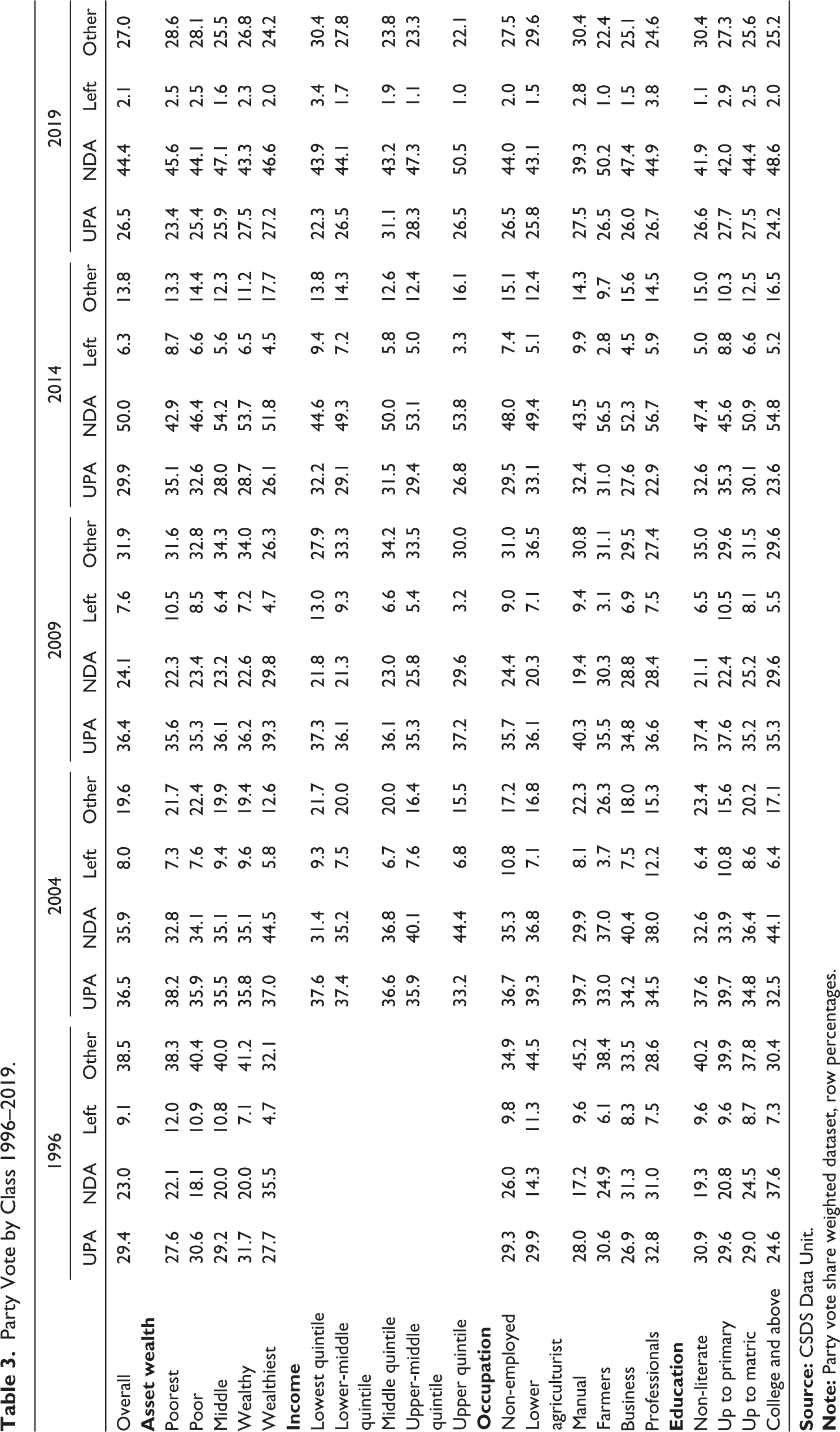
As per asset-wealth, the UPA was drawing its support roughly equally from nearly all asset classes in 1996–2004, whereas the wealthiest supported the NDA rather than the UPA consistently (except in 2009). In 2014, the UPA lost its support across class, retaining its support somewhat among the poorest more than among other classes. However, this support eroded further in 2019. The NDA saw an increase across asset classes (with a dip between 2004 and 2009), consolidating its vote share among the asset-poorer groups. Analysing by gender, in 1996–2009, except wealthy women, women from all other asset classes were more likely to vote for the UPA (2009 was an exception where wealthy women turned out overwhelmingly for the UPA). However, the pattern for women too swung in 2014 when women across all classes voted more for the NDA. Men displayed a similar pattern. The figures across locality were similar.
In terms of income, there was a pattern of the poorest supporting the UPA generally up until 2014, and the vote among the income poorest for the UPA was higher in 2014 than among other classes. In 2019, interestingly within the middle and upper-middle classes, there was a greater support for the UPA than other classes, and the poor seemed to be least supportive of the UPA, thus indicating a further loss of its traditional vote base. In 2014–2019, across all income classes, the support for the NDA was higher, though those in the richer quintiles had a higher support for them. The gender pattern by income quintiles were similar, except for 2004 when the middle- and higher-income groups of women were more likely to vote for the NDA than women of other classes (this reversed in 2009 and then returned back again in 2014). For men, it was the upper-middle and the upper quintiles who supported the NDA. Again, the patterns were similar by locality.
In terms of occupation, in the years of the UPA victory at the national level, the UPA was drawing its vote share consistently across occupations more than the NDA, with the exception of the business class and later the farming class. However, since 2014, across all occupational groups, the vote share for the NDA has been exceeding that for the UPA. The biggest shift to the NDA was among professional, business and farm-owning women in 2019. In urban India, the non-employed/homemakers were NDA supporters in 1996 (with a minor difference with the UPA in 2004; a higher difference in 2009), and then overwhelmingly in 2014 and 2019.
In terms of education, the patterns were quite distinct, with college and above educated consistently supporting the NDA more than the UPA (except in 2009). While the UPA vote share generally declined, the lower and middle educated were more likely to vote for it than were the more educated consistently across all years. We find some interesting patterns with women in intermediate/college supporting the UPA more than men with the same education. Among the non-literate, more women than men supported the NDA in 1996, equalising for the middle three survey periods, and reversing with more non-literate men supporting them in 2019. For the UPA, the pattern was not consistent, and nearly the opposite of that for the NDA, with more support for the UPA among non-literate women than men in 2019. The rural–urban patterns are similar.
Subjective/Self-Identified Class
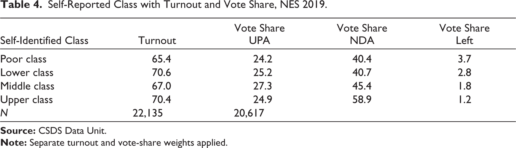
For 2019, an additional analysis using subjective class identification (Table 4) shows us that the highest turnout is for the self-identified lower and upper classes and not for the middle class. This is the opposite of patterns seen by income, asset-wealth and education and raises the question about what exactly the self-identified variable in the data is measuring. The support for the NDA increases with each level of subjective class (as does support for the UPA but at a lower level, except for the upper class which shows less support for the UPA than the middle and lower classes). The support for the left parties declines consistently with an increase in subjective class.
Self-Reported Class with Turnout and Vote Share, NES 2019.
Caste and Class Patterns
Prior work has shown a persisting association between caste and class, especially at the extremes (Vaid, 2018). One can expect that electoral participation may also display specific class-based patterns within each caste (see Jaffrelot, 2015). While this article does not study this relation in detail, this section provides a brief discussion of community/caste-based patterns within class using the 2019 NES data first as related to turnout and then with regard to vote share. 16
Disaggregating turnout by wealth (Table A12), for the UC (the so-called ‘upper castes’), the lowest turnout was for the asset-poorest, and among all other castes/communities, the lowest turnout was for the asset-wealthiest. For the UCs, Other Backward Castes (OBCs) and Schedule Tribes (STs), the highest turnout is the middle asset group; for the Schedule Tribes (SCs) and Others, it is the lower middle; and for Muslims, it is the poorest.
In terms of income also, the poorest UCs, STs and Others had the lowest turnout. For the OBCs, it was the upper-middle quintile; and for the SCs, Muslims and Others, it was the richest with the lowest turnout. The highest turnout for UC and OBC is for the lower-middle quintile, the middle quintile for the SCs and Muslims, and interestingly the richest for the STs who turned out more.
With regard to occupation, for the UC, the lowest turnout was for lower agriculture, manual work and professionals, and the highest was for farmers. For the Muslims and Others, the lowest turnout was for the professional occupations; for SC and ST, it is for manual work; and for OBCs, it was the non-employed/other. For UCs, OBCs and Others, the highest turnout was for the farmers; and for SCs, STs and Muslims, it was for the business class.
In terms of education, across caste and community, the lowest turnout was for the non-literate (for the SC in addition it was the up to matriculate), and for Others, it was the college and above. The highest turnout across caste by education was for the up to matriculate for the UCs and SCs, whereas for OBCs, STs and Muslims, it was the primary school educated with the highest turnout.
A separate paper would be needed to comment on the details of caste-wise disaggregation and party choice. However, there are some things that stand out when we look at community/caste and class disaggregation (Table A13) despite the overwhelming support for the NDA. The overall figures show that the UC have the highest support for the NDA (59.6%), followed by the OBCs (54.2%) and STs (45.4%). This contrasts with the support among the Muslims which is the lowest at 9.2%. Disaggregating these figures by class shows us how complex the picture truly is.
While the support for the NDA remains higher than that for the UPA at all asset-class levels within caste, the main exception is the wealthiest SCs who voted more for the UPA than the NDA, as did Muslims and Others. Further, the gap between UPA and NDA (in favour of the NDA) is smallest for the poorest STs, and highest among the poorest UCs. Also, among the UCs, the middle-asset quintile has the higher support for the NDA than other asset groups.
With regard to income, again we find that the richest SCs voted more for the UPA than the NDA. Further, the gap between the UPA and the NDA was narrowest for the middle-income quintiles for STs, though the vote for the NDA was consistently more than that for the UPA across all income classes (with the exception of the SCs mentioned). Muslims regardless of income voted more for the UPA as did the Other Minorities.
By occupation, we find a consistent preference for the NDA across occupation classes, with the exception of the Muslims and Other Minorities. Among the UC, among the farmers as compared to other classes, the support in favour of the NDA (the gap between the NDA and UPA votes) is larger; among the OBCs, this gap is larger for the business class; among SCs, it is for the lower agriculture; among STs, farmers have a higher support for the UPA, whereas the gap in favour of the NDA is highest among manual workers. While the Muslims have higher support for the UPA regardless of occupation, among the professionals, there is slightly more support for the NDA than among other occupations.
The support for the NDA exceeds that for the UPA across all disaggregations of education by community, except among Muslims and Others Minorities. Among the UCs, OBCs, SCs and STs, the lowest support for the NDA is among the non-literate. The patterns for the highest support vary—the highest educated among the UC, ST and to an extent Muslims support the NDA. Among the SCs, those with college and above education have higher support for the UPA (the gap between UPA and NDA is lower) than those with other levels of education.
The Impact of Class: Regression Analysis
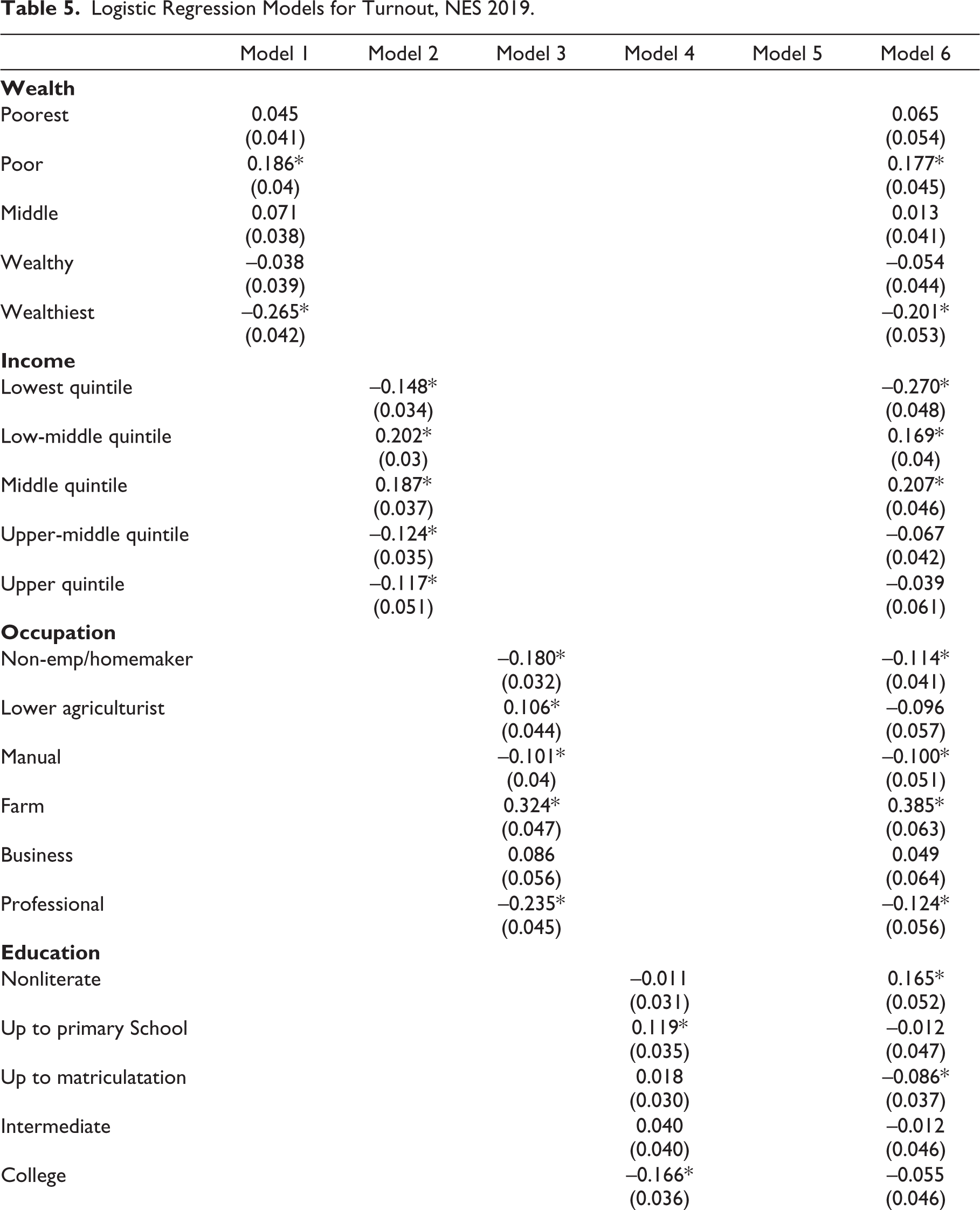
In the final analysis of this article to study the impact of different measures of class on turnout and vote for the NDA, we use binary logistic-regression models, with deviation contrasts. Deviation contrasts compare the parameter estimates to the ‘unweighted average of all groups’ (Nichols, 1997) and not to any specific reference group 17 (see Kumar et al. [2002] and Vaid and Heath [2010] for a discussion on treating these parameters as ‘fitted logs odds ratios’). Table 5 has the outcome variable of turnout (1 = voted, 0 = not voted), while Table 6 has vote for the NDA as outcome (1 = NDA vote, 0 = all other parties).
Model 1 in both tables controls for asset-wealth, model 2 for income, model 3 for occupation, model 4 for education and model 5 for self-identified class. Model 6 includes all the measures of class together. Each of these models also controls for caste/community, locality, gender, political interest and political participation (measures that were discussed earlier).
In Table 5, model 1, the asset-poor as compared to the average have more favourable relative chances of turning out to vote, and the wealthiest have the least favourable relative chances controlling for variables such as locality, gender, community and so on. In model 2, the extremes with the lowest income quintile and upper-middle and upper quintiles have the least favourable chances of turnout, whereas those in the middle have better chances than the average. In model 3, the farming categories have better, and all others have less, relative chances than the average. The business class is not statistically different from the average. Those with college and higher education turnout less (model 4) and those with primary schooling vote more. For model 5, the pattern in terms of subjective class is unclear—those who identify as middle and poor have less favourable chances of voting, and the lower and upper class have more favourable ones. In the complete model (6), with all the measures of class 18 and controls, most results remain similar overall (with minor differences); however, the parameters for education alter the most when other measures of class are controlled for. Controlling for all measures of class, the non-literate have more favourable relative odds to vote, and the up to matriculate have less favourable relative odds.
Logistic Regression Models for Turnout, NES 2019.
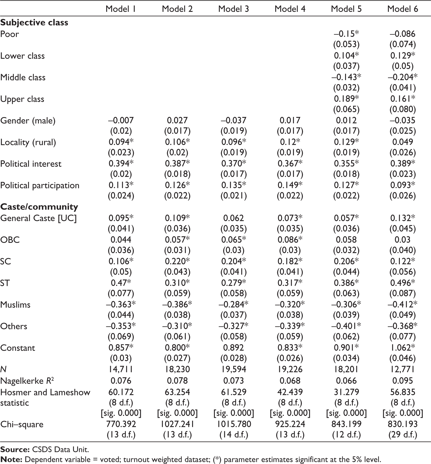
In all these models, gender is not statistically significant, people from rural areas turnout more, and those with higher political interest and participation have better relative chances of voting controlling for class. Caste/community figures vary slightly by model, but overall regardless of which measure of class one uses, Muslims and other religions have worse, and all others (General [UC], OBC, ST, SC) have better relative chances, to vote. While the Hosmer and Lameshow statistic does not fit the models, due to limitations of this test and the purpose of testing each measure of class, we interpret the models as a whole. As per the Nagelkerke R2 (which shows weak correlations between the independent variables and turnout), the best fitting model is the complete one (model 6) where 9.5% of the total variation in turnout is explained, followed by model 2 with income controls 19 and the least fitting model is where subjective class is used (6.6% of turnout is explained).
Moving on to regression models studying NDA vote in 2019, we see interesting patterns. According to asset-wealth (Table 6, model 1), controlling for gender, community etc., the poorest have better relative chances and the wealthy worse relative chances to vote for the NDA (the parameter estimates for the wealthiest and other classes are not statistically significant). However, in model 2, the upper-middle-income quintile is the only statistically significant parameter showing a higher relative chance of voting for the NDA. By occupation (model 3), business people and the non-employed/homemakers vote NDA, whereas lower-agriculturalists and manual workers do so less as compared to the average. None of the parameters for education are statistically significant. Finally, those in the highest subjective class are NDA supporters, while the lower and middle class have unfavourable relative chance of voting for the NDA (model 5).
Logistic Regression Models for NDA Vote, NES 2019.
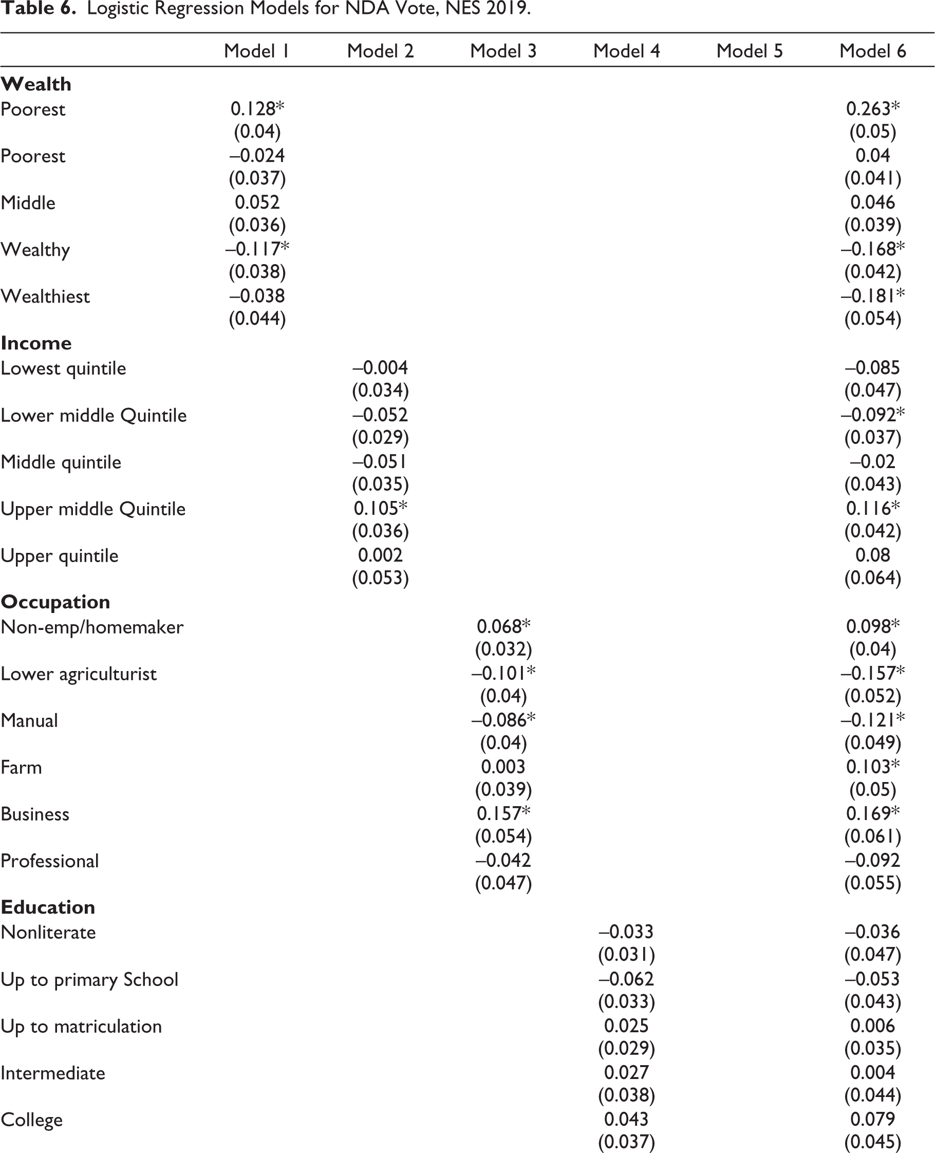

The controls in all the models show that regardless of the measure of class used, men have more favourable relative chances than the average, and those with more political interest are more favourable relative chances, to vote NDA. Interestingly, those with higher political participation have less favourable chances of voting for the NDA than the average. The results do not vary by locality. In terms of community/caste, in all models (controlling for class), we find that caste Hindus are NDA supporters, and Muslims and other religions are not.
The final model (6) controlling for all measures of class with other controls displays opposite results for wealth and income (similar to asset patterns)—the asset-poorest vote more for the NDA and the asset wealthy and wealthiest vote less, where the upper-middle-income class has more favourable chances of voting for the NDA and the lower-middle quintile has unfavourable chances. Lower agriculturalists and manual workers are less likely to vote for the NDA, and business people and homemakers/non-employed are more likely to do so. As per subjective-class, higher classes support the NDA more than the average class. The results for education are not statistically significant. The best fitting model is the full one, followed by the model controlling for subjective class.
Overall, except for asset-wealth, the picture is that the more well-off have relatively favourable chances of voting for the NDA. This exception of wealth from the overall patterns is important to keep in mind, especially because studies have conflated asset and income in creating class indices.
Conclusion
This article set out to study whether patterns of turnout and vote share vary across measures of class. Further, it asked whether these measures of class have a similar impact on turnout and vote share. This study is significant given the confusion in measuring class in the study of electoral participation in India, where indexes bringing together component measures of class such as income, assets and occupation in inconsistent ways provide divergent results. If the substantive focus of any study is on class, then defining and operationalising class is crucial. As a first step in this direction, this article studied asset-wealth, income, occupation and education separately in relation to electoral participation between the 1996 and 2019 general elections. Further, as these patterns themselves are aggregates, the paper disaggregated them by gender, locality and caste/community.
This section summarises some of the broader patterns and discusses their implications.
First, with regard to turnout, those in the middle range of two measures, asset-wealth and income, are more likely to turnout over the years; however, the 2014 election has seen an upswing in voting across all class categories, which was surpassed in 2019. Interestingly, in the last two general elections, it is the asset-poorest (and the lower-middle) who are turning out to vote more than those in the upper-middle and wealthy categories. For education, we do not observe any consistent pattern, though an increase overall is seen in the last two elections, with the lowest turnout for the non-literates. According to occupation before 2014, the highest turnout was for the business class, followed by farmers, lower agriculturalists, manual workers and professionals, while the lowest was for the non-employed/homemakers. In 2019, it is the two farm categories with the highest turnout, followed by business, manual, non-employed/homemakers, with professionals with the lowest turnout. The gender-wise comparison leads us to conclude that more women are turning out to vote over time, and the odds of a woman voting compared to a man has indeed improved over the five election years. With regard to asset-wealth, the odds ratios are highest for the middle and the lower middle class, which implies that there are more equal chances for women from these classes to vote than men. The odds ratios for the two wealthiest categories imply a more unequal gender turnout. This pattern holds for income. In terms of occupation, manual work in particular displays a favourable gender odds ratio across the years. Interestingly, the gender odds ratio is worst for the highest level of education in all years. The figures by locality are less distinct, though the rural turnout is consistently higher than the turnout in urban areas across all measures of class. Subjective class patterns for 2019 are the opposite of income, wealth and education patterns, where rather than the middle class, the highest turnout is for the poorest and the upper classes.
Second, with regard to vote share for the two largest alliances, 2014 stands out with the large upswing for the NDA across all measures of class which is maintained in 2019. Further, over time the vote for the NDA comes from the wealthiest and most educated voters, though the lowest income and asset groups have increased their vote share for it. Also, while the UPA’s vote share generally declined, the lower and middle educated groups were more likely to vote for it than were the more educated across the years.
Third, disaggregation by caste underlines the intersection between class and caste. For the UCs and OBCs, the highest turnout is for the middle asset group, the lower-middle-income group, farmers and those with middle levels of education. The patterns for the other caste groups are less consistent, though for the SCs and Muslims, the lower middle and lowest asset group (respectively) and the middle-income group have the highest turnout. In terms of party-vote, while the UCs, followed by the OBCs, and STs have the highest support for the NDA, the class disaggregated analysis shows a complicated picture. The asset-wealthiest and income-richest SCs voted more for the UPA as did Muslims regardless of class. In contrast, among the UCs, the middle asset group, the upper-middle and richest groups, farmers and the most educated had the most support for the NDA.
Finally, the regression analysis emphasises some of this variation further, especially concluding that different measures of ‘class’ show different results. In terms of the impact of caste controlling for measures of class, we find that UC Hindus have relatively higher support for the NDA and Muslims do not. Overall, controlling for caste (and other controls), the upper-middle income, the business and the higher subjective classes have relatively favourable chances of voting for the NDA; the exception here are the asset-poor who also have favourable relative chances of NDA vote.
The implications of these broad findings are twofold: substantive and methodological.
Substantively, we find some consistency in class-based participation/vote for asset-wealth and income (and to a lesser extent for education), but not so much for occupation, and with no distinct pattern with regard to party vote. We find an upsurge in turnout for the asset-poorest in the last two elections, which talks to the possibility of a democratic upsurge (Yadav, 2000). However, regarding income, we find an increase in turnout among the middle and upper categories, which talks more to a levelling off (Kumar, 2009), as does the increase in women’s turnout among the middle and upper classes. Further, while the rural turnout exceeds the urban, we find a levelling with those in wealthier income and asset groups and in higher education increasing their turnout in urban India. Overall, the picture across class is inconsistent.
Further, studying what factors may be driving an upsurge among groups such as the asset-poorest, requires elaboration in the light of possible pro-poor policies and their impact (see Sridharan, 2014), which was outside the present study’s scope. Similarly, in order to understand why we find a particular pattern of vote among the UC/OBC which have greater support in the middle for the NDA, and the higher support for the UPA among upper-class SCs, we would need to study specific welfare policies and provide a more historically contextual view of party support bases.
Methodologically, the lack of consistency in findings across measures of class is a warning about creating class indices without considering what exactly is being measured, whether it is being measured at the individual (occupation/education) or household (income/asset) level, whether it is being measured at the ordinal (education/asset), interval (income) or nominal (occupation) level and the implications of this on the class construct and the results. Any future work using class would benefit by considering the heterogeneities of the indicators used to measure class.
Footnotes
Acknowledgements
I thank the Lokniti–CSDS Data Unit for access to their database, and I am grateful for the review comments and suggestions received on an earlier draft of this article.
Declaration of Conflicting Interests
The author declared no potential conflicts of interest with respect to the research, authorship and/or publication of this article.
Funding
The author received no financial support for the research, authorship and/or publication of this article.