Wealth Inequality and Carbon Emissions in High-income Countries

Abstract

This study contributes to the emerging literature on connections between climate change and economic inequality by investigating the relationship between domestic wealth inequality and consumption-based carbon emissions for 26 high-income countries from 2000 to 2010. Results of the two-way fixed effects longitudinal models indicate that the effect of wealth inequality, measured as the wealth share of the top decile, on per capita emissions in high-income countries is consistently positive and relatively stable over the time period. This finding is consistent with political economy theories arguing that the concentration of political and economic power that accompanies the concentration of wealth plays an important role in increasing environmental degradation and preventing proenvironmental actions.

Keywords

climate change carbon emissions inequality environment

Introduction

As the problems of climate change and rising economic inequality become more urgent, greater scholarly attention is being paid to the ways in which they are interrelated (e.g., Chancel and Piketty 2015). One line of research in environmental sociology has begun to examine the effects of domestic economic inequality on anthropogenic carbon dioxide emissions using data at national and sub-national scales (e.g., Jorgenson et al. 2015; Jorgenson et al. 2016; Jorgenson et al. 2017). A deeper understanding of this relationship could facilitate policies aimed at addressing economic inequality that also mitigate emissions, and vice versa (Kenner 2016).

Previous cross-national research on the domestic inequality/emissions relationship has yielded mixed results. Early studies, focusing on Gini coefficients and varied propensities to consume carbon-intensive goods across income classes, found a negative association between income inequality and carbon emissions (Heerink, Mulatu, and Bulte 2001; Ravallion, Heil, and Jalan 2000). However, later research suggested a nonsignificant relationship (Borghesi 2006; Gassebner, Lamla, and Sturm 2011). A subsequent study of 138 countries between 1960 and 2008 found a U-shaped relationship between income inequality and emissions, where rising inequality reduces emissions in more equal countries and raises them in more unequal countries (Grunewald et al. 2012). The inflection point is at a higher level of inequality for poorer than wealthier countries, suggesting that income redistribution could reduce emissions in wealthy countries with high income inequality, but is unlikely to do so in poorer countries. More recently, Jorgenson et al. (2016) analyzed the impact of income inequality on consumption-based carbon emissions for 67 countries from 1991 to 2008. They found that the effect of income inequality on emissions became increasingly positive in higher income nations, and that the income level of countries also affects the relationship. Jorgenson et al. (2015) also analyzed the relationship between U.S. state-level residential carbon emissions and income inequality (measured as the Theil index) for the 1990 to 2012 period, finding a positive association, while Jorgenson et al. (2017) found that U.S. state-level emissions from all sectors combined was positively associated with the income share of the top 10 percent, top 5 percent, and top 1 percent during the 1997 to 2012 period.

A limitation of these studies is that they all focus on income inequality and fail to consider the role of wealth inequality.¹ We suggest that a more comprehensive understanding of the inequality/emissions relationship requires examining both dimensions of economic inequality. As many scholars have argued, there are important differences in the causes and consequences of income and wealth inequality (Keister and Lee 2014; Piketty 2014, 2015). Furthermore, wealth is more unequally distributed than income (Kus 2016) and, according to a recent analysis of 17 Organisation for Economic Co-operation and Development (OECD) countries, income inequality and wealth inequality are only weakly related (OECD 2015). Therefore, it cannot be assumed that these two dimensions of economic inequality have similar effects on carbon emissions.

With the exception of Jorgenson et al. (2016), another limitation of the foregoing research is the use of territorial (or production-based) carbon emissions that only reflect emissions originating within a country. However, measures of consumption-based emissions, which adjust for emissions transfers via international trade (i.e., adding in emissions embodied in imports and subtracting emissions embodied in exports), are important to consider as production and consumption activities are increasingly spatially separated in the global economy (Peters et al. 2011). Consumption-based emissions provide a more comprehensive accounting of the contribution of each country to global climate change and thus are more appropriate for assessing the various potential effects of wealth inequality on environmental degradation.

We advance this line of research by investigating the relationship between consumption-based carbon emissions and domestic wealth inequality for a sample of 26 high-income nations for the 2000 to 2010 period. We allow the effect of wealth inequality to vary over time, a dynamic that has been observed for other anthropogenic drivers of emissions, such as economic development and urbanization (e.g., Jorgenson, Auerbach, and Clark 2014; Jorgenson and Clark 2012; Knight and Schor 2014).

Theoretical Linkages

Social scientists have theorized multiple pathways through which domestic economic inequality may affect carbon emissions (for a thorough review, see Cushing et al. 2015). Inequality may inhibit proenvironmental collective action and socially responsible behaviors by eroding social trust, cohesion, and cooperation, which can result in greater environmental degradation, including increased emissions, as environmental problems are not effectively met by changes in individual behavior or public policy (Boyce 2003; Cushing et al. 2015; Ostrom 2008; Sonderskov 2008; Wilkinson and Pickett 2010). Experimental research suggests that economic inequality impedes cooperation to reduce emissions when the poor are more vulnerable to the negative consequences of climate change (Burton-Chellew, May, and West 2013). In addition, higher economic inequality has been found to be associated with increased competitive status-based consumption and longer working hours, both of which are positively associated with energy consumption and carbon emissions (Bowles and Park 2005; Cushing et al. 2015; Fitzgerald, Jorgenson, and Clark 2015; Knight, Rosa, and Schor 2013; Schor 1998). Thus, greater income and wealth inequality may shape consumer and labor market dynamics in ways that increase emissions by spurring status competition as the wealthy set higher and higher standards for consumption.

In contrast, it has also been suggested that higher income inequality may actually be associated with lower emissions, because the marginal propensity to emit (and consume) declines with income (Heerink et al. 2001; Ravallion et al. 2000). This argument suggests that attempts to reduce economic inequality could result in increased emissions as income is redistributed to the poor.

Perhaps most relevant for wealth inequality, however, is the political economy approach introduced by James Boyce (1994), and further developed by Downey (2015), which links economic inequality to environmental degradation via the unequal distribution of power. We highlight the mechanism of power, rather than the other linkages discussed above because the others may be more influenced by income than wealth. Though wealth can affect consumption, these “wealth effects” are generally considered small in comparison with the impact of income (e.g., Sierminska and Takhtamanova 2007). By contrast, wealth is more likely to be an indicator of power. As Winters and Page (2009) argued, more so than income, wealth is translatable to political influence and power in that it is “a material form of power that is distinct from all other power resources, and which can be readily deployed for political purposes” (p. 732).

Boyce’s (1994, 2003, 2008) political economy framework centers on what he termed the “power-weighted social decision rule,” which specifies that when the beneficiaries of environmental degradation are more powerful than those who bear the costs, the overall level of environmental degradation will be greater. Because the affluent benefit more from environmental degradation (as both producers and consumers) while the poor benefit less and are more vulnerable to the harmful consequences (e.g., pollution, proximity to industrial activities), greater economic inequality is likely to lead to increased environmental degradation as the interests of the affluent are protected in the political realm (Cushing et al. 2015). Consistent with this argument, research from the United States indicates that the wealthiest are less supportive of environmental protection and also disproportionately participate in politics (Page, Bartels, and Seawright 2013; Page and Hennessy 2011). Furthermore, numerous environmental justice studies demonstrate empirically that lower income neighborhoods and communities are disproportionately exposed to environmental hazards (Brulle and Pellow 2006; Mohai, Pellow, and Roberts 2009). In their study of air pollution in metropolitan areas of the United States, Ash et al. (2013) found evidence consistent with Boyce’s theory that where environmental inequality is more pronounced, the overall level of environmental degradation is greater. Climate change is not spatially localized and thus may not seem to be subject to the dynamics described by Boyce, but some research has found otherwise. Pattison, Habans, and Clement (2014) demonstrated that the higher income counties in the United States have greater consumption-based carbon emissions but lower production-based emissions than lower income counties, which suggests that “The most affluent localities have the power to displace carbon-intensive industrial activities onto less affluent communities” (p. 862).

In environmental sociology, Downey’s (2015) inequality, democracy, and environment (IDE) model synthesizes and builds on the work of Boyce (1994, 2008), Schnaiberg’s (1980) treadmill of production theory, and ecologically oriented world-systems theory (e.g., Roberts and Grimes 2002) to draw connections between inequality, elite power, and the environment. The IDE model specifies the mechanisms by which organizational, institutional, and network-based inequalities lead to environmental degradation. Downey (2015) argued that elites actively work to create undemocratic institutions and elite-controlled organizations and networks as means to exert their power and achieve what are often environmentally destructive goals. He identified several ways that inequality can exacerbate environmental degradation, such as concentrating decision-making power, shifting environmental costs to those who are less powerful and less affluent, inhibiting public environmental concern and circumscribing proenvironmental behaviors, and enhancing the ability of elites to frame issues in their favor and divert attention from their activities (Downey 2015; Downey and Strife 2010).

The political economy approaches of Boyce and Downey are particularly relevant for studying the wealth inequality/emissions relationship because of the political character of wealth. As Winters and Page (2009) note, “concentrated wealth in the hands of a small fraction of a community’s members is a particularly versatile and potent source of political power” (p. 732). Political power derived from concentrated wealth can be exercised without much individual effort as the wealthy often control organizations and companies or have the means to hire professionals and firms that can act for them in the pursuit of their interests (Winters and Page 2009). To the degree that wealth inequality is tied to political inequality, the political economy approach suggests that environmental harms, including carbon emissions, will be greater when wealth is more unequally distributed.

Data and Method

The dependent variable in the present study is consumption-based carbon dioxide emissions in metric tons per capita, and includes emissions from fossil-fuel combustion, cement production, and gas flaring, but not those from bunker fuels used in international transport or land use and cover change. These data are also referred to as trade-adjusted carbon emissions as they account for the emissions generated in the processes of production, which are then attributed to the consuming (i.e., importing) rather than producing (i.e., exporting) country using input-output analysis. In contrast, data on territorial (production-based) emissions include only emissions that occur within a country (i.e., domestic production plus exports; see Peters 2008). In developed countries, consumption-based emissions tend to be greater than territorial emissions, and emissions embodied in trade are on the rise. However, the biggest contributor to consumption-based emissions in most countries is territorial emissions from domestic production that is consumed domestically (Peters, Davis, and Andrew 2012). Since the potential effects of economic inequality on environmental degradation (as identified in previous research and theorization) encompass both production and consumption dynamics, we prefer to use the more comprehensive consumption-based emissions measure. We obtain these data from the online database of the Global Carbon Atlas (http://www.globalcarbonatlas.org/). Our use of these data is consistent with prior cross-national research in environmental social science (Jorgenson et al. 2016; Knight and Schor 2014; Lamb et al. 2014). For additional details on the methodology involved in creating these measures, see Le Quéré et al. (2013) and Peters et al. (2011). For a useful assessment of the robustness and reliability of estimates of consumption-based emissions, see Peters et al. (2012).

The main independent variable is wealth inequality, which is measured as the wealth (i.e., individual net worth) share (percentage) of the top decile of adults aged 20 and up in each country, that is, the percentage of total wealth owned by the top 10 percent of wealth holders. Measuring inequality as the concentration of wealth at the top of the distribution is particularly suitable for evaluating the political economy approaches given the political implications of highly concentrated wealth (Jorgenson et al. 2015; Winters and Page 2009).² These data are from Table 4-4 in the 2014 Credit Suisse Global Wealth Databook (Shorrocks, Davies, and Lluberas 2014). Shorrocks et al. (2014) estimated the wealth share of the top decile in each country by using household balance sheet data, regression estimates, and rich lists, such as those published by Forbes Magazine (to more accurately depict the extreme upper tail of the wealth distribution). Because of the unavailability or incompleteness of wealth data for certain countries and the potential for error in these estimates, we conservatively limit our analysis to countries rated by Shorrocks et al. (2014) as having “good” or “satisfactory” quality wealth distribution data.³ We use interactions between wealth inequality and dummy variables for each year (2000–2010), with 2000 as the reference year, which allow for assessing the extent to which the effect of wealth inequality on emissions increases or decreases through time (Allison 2009). A balanced panel dataset is preferable for such an analysis (e.g., Jorgenson and Clark 2012), which along with data availability, limited the countries and years that could be included in the study.

Control variables include gross domestic product (GDP) per capita and income inequality.⁴ GDP per capita is measured in constant 2005 U.S. dollars from the World Bank’s online World Development Indicators Database (http://databank.worldbank.org/data/home.aspx). In line with previous research, income inequality is measured as the Gini coefficient of inequality for household disposable income (posttax, posttransfer), taken from Solt’s Standardized World Income Inequality Database (Version 4, http://myweb.uiowa.edu/fsolt/swiid/swiid.html; see also Solt 2009). Table 1 reports descriptive statistics for all variables.

Table 1.

Descriptive Statistics.

Variable	Mean/Standard deviation
Carbon dioxide emissions per capita	1.08/.14
Wealth inequality	1.77/.05
Wealth inequality × 2001	0.16/.51
Wealth inequality × 2002	0.16/.51
Wealth inequality × 2003	0.16/.51
Wealth inequality × 2004	0.16/.51
Wealth inequality × 2005	0.16/.51
Wealth inequality × 2006	0.16/.51
Wealth inequality × 2007	0.16/.51
Wealth inequality × 2008	0.16/.51
Wealth inequality × 2009	0.16/.51
Wealth inequality × 2010	0.16/.51
GDP per capita	4.50/.20
Income inequality	1.48/.07
No. of nations/sample size	26/286

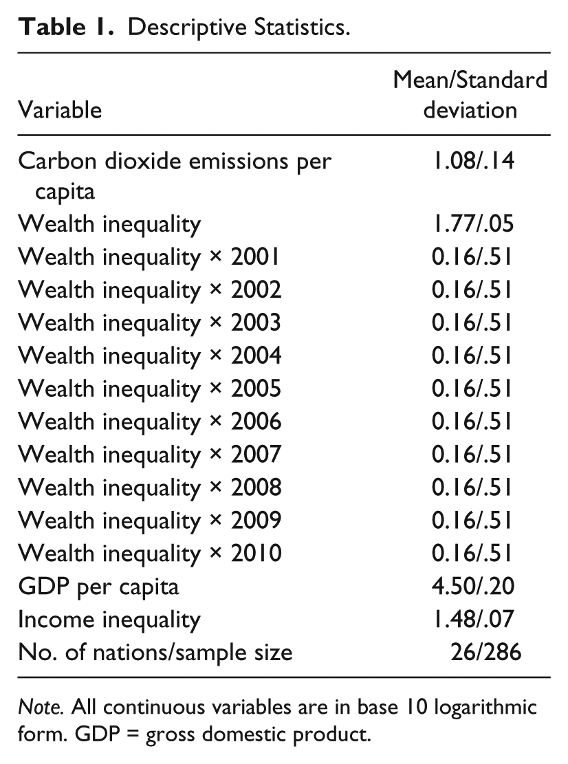
Note. All continuous variables are in base 10 logarithmic form. GDP = gross domestic product.

Our sample consists of a balanced panel dataset of annual observations from 2000 to 2010 for 26 high-income countries (N = 286).⁵ Limiting the analysis to countries with “good” or “satisfactory” quality wealth distribution data (according to Shorrocks et al. 2014) restricts the number of countries to 28 (excluding Taiwan for which data on the control variables are not available). All but two of these countries are classified as high-income (in 2010) by the World Bank. Because prior research suggests the economic inequality/emissions varies by levels of economic development, we excluded the two non-high-income countries (Colombia and Mexico) from the analysis, which results in a sample of 26 high-income countries (Grunewald et al. 2012; Jorgenson et al. 2016).

Consistent with prior research, we use a time-series cross-sectional Prais-Winsten regression model with panel-corrected standard errors, allowing for disturbances that are heteroskedastic and contemporaneously correlated across panels (e.g., Jorgenson et al. 2016; Knight and Schor 2014). We correct for AR(1) disturbances (first-order autocorrelation) within panels and treat the AR(1) process as common to all panels (Beck and Katz 1995). We include dummy variables to control for both country-specific and year-specific effects, the equivalent of a two-way fixed effects model. This modeling technique controls out between-country variation in favor of estimating within-country effects, a relatively conservative approach for hypothesis testing. All variables are transformed into logarithmic form (base 10). Thus, the models estimate elasticity coefficients where the coefficient for the independent variable is the estimated net percentage change in the dependent variable associated with a 1 percent increase in the independent variable.

Results

Results for the analysis are reported in Table 2. Model 1 is the baseline model without interactions, in which the estimated elasticity coefficient of wealth inequality is significant and positive (b = .795) for the entire time period, indicating that a 1 percent increase in wealth inequality is associated with a .795 percent increase in emissions per capita. Model 2 includes the interactions between wealth inequality and dummy variables for each year to test whether the relationship between wealth inequality and emissions changes over time.

Table 2.

Prais-Winsten Regression Two-Way Fixed Effects Elasticity Model of the Effects of Wealth Inequality on Per Capita Consumption–Based Carbon Dioxide Emissions, 2000–2010.

	Model 1	Model 2
Wealth inequality	.795** (.304)	.840** (.302)
Wealth inequality × 2001		−.075 (.042)
Wealth inequality × 2002		−.168*** (.046)
Wealth inequality × 2003		.032 (.043)
Wealth inequality × 2004		−.087* (.040)
Wealth inequality × 2005		−.084* (.039)
Wealth inequality × 2006		−.122** (.040)
Wealth inequality × 2007		−.060 (.045)
Wealth inequality × 2008		−.030 (.046)
Wealth inequality × 2009		−.100* (.044)
Wealth inequality × 2010		−.011 (.043)
GDP per capita	.390** (.138)	.379** (.140)
Income inequality	−.145 (.181)	−.154 (.184)
R ²	.9716	.9722
No. of nations/sample size	26/286	26/286
No. of coefficients	39	49
ρ	.410	.406

Note. Panel-corrected standard errors are in parentheses. All continuous variables are in base 10 logarithmic form. Models include unreported unit-specific and period-specific intercepts (two-way fixed effects). GDP = gross domestic product.

p < .05. **p < .01. ***p < .001 (two-tailed tests).

In Model 2, the estimated elasticity coefficient of wealth inequality in 2000 (the reference year and determined by the main effect) is positive and significant (b = .84), indicating that a 1 percent increase in wealth inequality in 2000 is associated with a .84 percent increase in emissions per capita. The effect of wealth inequality for the other time points (i.e., 2001, . . ., 2010) equals the sum of the coefficient for wealth inequality in 2000 and the appropriate interaction term if the latter is statistically significant (Allison 2009). For the years 2002, 2004, 2005, 2006, and 2009, the interactions are negative and statistically significant, but for the other five years, the interactions are nonsignificant. To ease interpretation, Figure 1 provides the estimated yearly effects of wealth inequality on emissions (based on the estimated elasticity coefficients in Table 2). The estimates show that though there is some fluctuation from year to year, there is no steady increase or decrease in the size of the effect of wealth inequality on emissions. The elasticity coefficient of wealth inequality ranges from a low of 0.672 to a high of 0.84 over this period. Overall, the results suggest that the effect of wealth inequality on emissions in high-income countries is positive and relatively stable over time, though it may vary somewhat in magnitude.

Figure 1.

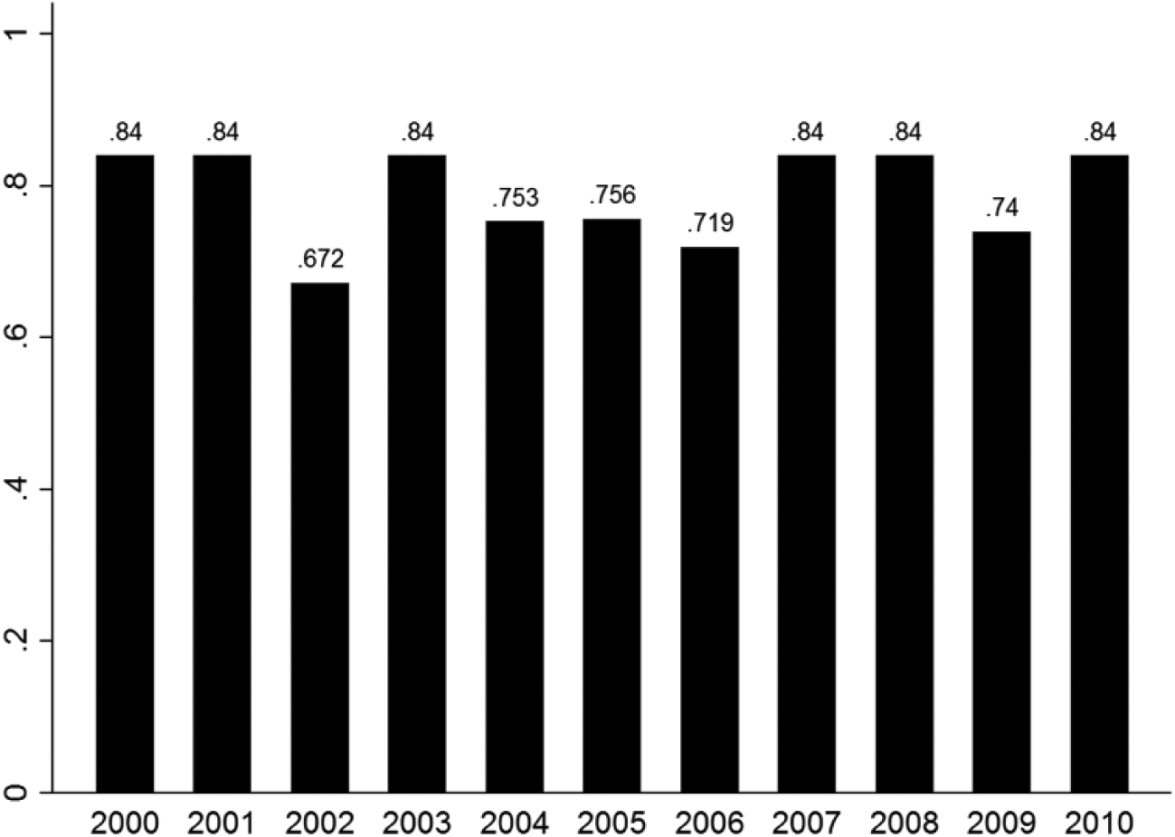
Estimated effects (elasticity coefficients) of domestic wealth inequality on per capita consumption–based CO₂ emissions, 2000–2010.

Turning to the control variables, the coefficient for GDP per capita is positive and significant, which is consistent with prior research (e.g., Jorgenson and Clark 2012). The coefficient for income inequality is nonsignificant, which is consistent with the findings of Borghesi (2006) and Gassebner et al. (2011) but less so with Jorgenson et al. (2016) and Grunewald et al. (2012).⁶ Our results suggest that inequality in wealth, measured as concentration at the top of the distribution, may be more important in predicting emissions than income inequality, at least when the latter is measured with the Gini coefficient.

Conclusion

Environmental sociologists have long focused on the ways in which power and inequality shape society-environment interactions (Pellow and Brehm 2013). Therefore, it is somewhat surprising that connections between domestic economic inequality and carbon emissions have largely been overlooked until recently (Jorgenson et al. 2015; Jorgenson et al. 2016; Jorgenson et al. 2017). With the goal of advancing this nascent literature, the present study focused on estimating the effect of wealth inequality (measured as the wealth share of the top decile), on consumption-based carbon emissions. We found that in high-income countries, wealth inequality has a relatively stable positive effect on emissions over the 2000 to 2010 period. This finding is consistent with political economy theories arguing that the concentration of power that accompanies the concentration of wealth plays an important role in intensifying environmental degradation (Boyce 1994, 2003, 2008; Downey 2015; Downey and Strife 2010). It is important to note, however, that the present study is limited in that it does not identify the specific mechanism(s) that may link wealth inequality to emissions, but only empirically demonstrates an association between the two. The results also indicate that the effect of income inequality, measured as the Gini coefficient, is nonsignificant. This suggests a need for more research on both dimensions of economic inequality and to explore different inequality measures. However, limited availability of quality data on wealth and income inequality for many countries and years remains a problem. As more and better data become available, it will be necessary to revisit and refine research on this topic. Such research is especially important given that the findings of this study suggest that policies aimed at reducing wealth concentration could potentially yield a “double-dividend” in terms of social and environmental benefits.

Footnotes

Declaration of Conflicting Interests

The author(s) declared no potential conflicts of interest with respect to the research, authorship, and/or publication of this article.

Funding

The author(s) received no financial support for the research, authorship, and/or publication of this article.

Notes

References

Allison

Paul

. 2009. Fixed Effects Regression Models. Thousand Oaks, CA: Sage Publications.

Ash

Michael

Boyce

James

Chang

Grace

Scharber

Helen

. 2013. “Is Environmental Justice Good for White Folks? Industrial Air Toxics Exposure in Urban America.” Social Science Quarterly 94(3):616–36.

Beck

Nathaniel

Katz

Jonathan

. 1995. “What to Do (and Not Do) with Time-series Cross-section Data.” American Political Science Review 89:634–47.

Borghesi

Simone

. 2006. “Income Inequality and the Environmental Kuznets Curve.” Pp. 33–51 in Environment, Inequality, and Collective Action, edited by Basili

Marcello

Franzini

Maurizio

Vercelli

Alessandro

. New York: Routledge.

Bowles

Samuel

Park

Yongjin

. 2005. “Emulation, Inequality, and Work Hours: Was Thorsten Veblen Right?” The Economic Journal 115(507): F397–412.

Boyce

James

. 1994. “Inequality as a Cause of Environmental Degradation.” Ecological Economics 11:169–78.

Boyce

James

. 2003. “Inequality and Environmental Protection.” Working Paper No. 52, Political Economy Research Institute, University of Massachusetts, Amherst, MA.

Boyce

James

. 2008. “Is Inequality Bad for the Environment?” Research in Social Problems and Public Policy 15:267–88.

Brulle

Robert

Pellow

David

. 2006. “Environmental Justice: Human Health and Environmental Inequalities.” Annual Review of Public Health 27:103–24.

10.

Burton-Chellew

Maxwell

May

Robert

West

Stuart

. 2013. “Combined Inequality in Wealth and Risk Leads to Disaster in the Climate Change Game.” Climatic Change 120:815–30.

11.

Chancel

Lucas

Piketty

Thomas

. 2015. Carbon and Inequality: From Kyoto to Paris. Paris, France: Paris School of Economics.

12.

Cushing

Laura

Morello-Frosch

Rachel

Wander

Madline

Pastor

Manuel

. 2015. “The Haves, the Have-nots, and the Health of Everyone: The Relationship between Social Inequality and Environmental Quality.” Annual Review of Public Health 36:193–209.

13.

Downey

Liam

. 2015. Inequality, Democracy, and the Environment. New York: New York University Press.

14.

Downey

Liam

Strife

Susan

. 2010. “Inequality, Democracy, and the Environment.” Organization & Environment 23:155–88.

15.

Fitzgerald

Jared

Jorgenson

Andrew

Clark

Brett

. 2015. “Energy Consumption and Working Hours: A Longitudinal Study of Developed and Developing Nations, 1990–2008.” Environmental Sociology 1:213–23.

16.

Gassebner

Martin

Lamla

Michael

Sturm

Jan-Egbert

. 2011. “Determinants of Pollution: What Do We Really Know?” Oxford Economic Papers 63:568–95.

17.

Grunewald

Nicole

Klasen

Stephan

Martínez-Zarzoso

Immaculada

Muris.

Chris

2012. “Income Inequality and Carbon Emissions.” Discussion Paper No. 92, Courant Research Centre, University of Göttingen, Göttingen, Germany.

18.

Heerink

Nico

Mulatu

Abay

Bulte

Erwin

. 2001. “Income Inequality and the Environment: Aggregation Bias in Environmental Kuznets Curves.” Ecological Economics 38:359–67.

19.

Jorgenson

Andrew

Auerbach

Daniel

Clark

Brett

. 2014. “The (De-) Carbonization of Urbanization, 1960–2010.” Climatic Change 127:561–75.

20.

Jorgenson

Andrew

Clark

Brett

. 2012. “Are the Economy and the Environment Decoupling? A Comparative International Study, 1960–2005.” American Journal of Sociology 118:1–44.

21.

Jorgenson

Andrew

Schor

Juliet

Huang

Xiaorui

. 2017. “Income Inequality and Carbon Emissions in the United States: A State-Level Analysis, 1997–2012.” Ecological Economics 134:40–48.

22.

Jorgenson

Andrew

Schor

Juliet

Huang

Xiaorui

Fitzgerald

Jared

. 2015. “Income Inequality and Residential Carbon Emissions in the United States: A Preliminary Analysis.” Human Ecology Review 22(1):93–105.

23.

Jorgenson

Andrew

Schor

Juliet

Knight

Kyle

Huang

Xiaorui

. 2016. “Domestic Inequality and Carbon Emissions in Comparative Perspective.” Sociological Forum 31(S1):770–86.

24.

Keister

Lisa

Lee

Hang Young

. 2014. “The One Percent: Top Incomes and Wealth in Sociological Research.” Social Currents 1(1):13–24.

25.

Kenner

Dario

. 2016. Reducing Inequality and Carbon Footprints within Countries. Cambridge, England: Global Sustainability Institute, Anglia Ruskin University.

26.

Knight

Kyle

Rosa

Eugene

Schor

Juliet

. 2013. “Could Working Less Reduce Pressures on the Environment? A Cross-national Panel Analysis of OECD Countries, 1970–2007.” Global Environmental Change 23:691–700.

27.

Knight

Kyle

Schor

Juliet

. 2014. “Economic Growth and Climate Change: A Cross-national Analysis of Territorial and Consumption-based Carbon Emissions in High-income Countries.” Sustainability 6:3722–31.

28.

Kus

Basak

. 2016. “Wealth Inequality: Historical Trends and Cross-national Differences.” Sociology Compass 10(6):518–29.

29.

Lamb

William F.

Steinberger

Julia K.

Bows-Larkin

Alice

Peters

Glen P.

Roberts

Timmons J.

Wood

Ruth F.

2014. “Transitions in Pathways of Human Development and Carbon Emissions.” Environmental Research Letters 9(014011).

30.

Le Quéré

Andres

R. J.

Boden

Conway

Houghton

R. A.

House

J. I.

Marland

Peters

G. P.

van der Werf

G. R.

Ahlstrom

Andrew

R. M.

Bopp

Canadell

J. G.

Ciais

Doney

S. C.

Enright

Friedlingstein

Huntingford

Jain

A. K.

Jourdain

Kato

Keeling

R. F.

Klein Goldewijk

Levis

Levy

Lomas

Poulter

Raupach

M. R.

Schwinger

Sitch

Stocker

B. D.

Viovy

Zaehle

Zeng

2013. “The Global Carbon Budget 1959–2011.” Earth System Science Data 5:165–85. doi:10.5194/essd-5-165-2013

31.

Mohai

Paul

Pellow

David

Roberts

Timmons

. 2009. “Environmental Justice.” Annual Review of Environmental Resources 34:404–30.

32.

Organisation for Economic Co-operation and Development. 2015. In It Together: Why Less Inequality Benefits All. Paris, France: Organisation for Economic Co-operation and Development.

33.

Ostrom

Elinor

. 2008. “Frameworks and Theories of Environmental Change.” Global Environmental Change 18:249–52.

34.

Page

Benjamin

Bartels

Larry

Seawright

Jason

. 2013. “Democracy and the Policy Preferences of Wealthy Americans.” Perspectives on Politics 11(1):51–73.

35.

Page

Benjamin

Hennessy

Cari Lynn

. 2011. “What Affluent Americans Want from Politics.” Working Paper No. 11-08, Institute for Policy Research, Northwestern University, Evanston, IL.

36.

Pattison

Andrew

Habans

Robert

Clement

Matthew

. 2014. “Ecological Modernization or Aristocratic Conservation? Exploring the Impact of Affluence on Carbon Emissions at the Local Level.” Society & Natural Resources 27:850–66.

37.

Pellow

David

Brehm

Holly Nyseth

. 2013. “An Environmental Sociology for the Twenty-first Century.” Annual Review of Sociology 39:229–50.

38.

Peters

Glen

. 2008. “From Production-based to Consumption-based National Emission Inventories.” Ecological Economics 65:13–23.

39.

Peters

Glen

Minx

Jan

Weber

Christopher

Edenhofer

Ottmar

. 2011. “Growth in Emission Transfers via International Trade from 1990 to 2008.” Proceedings of the National Academy of Sciences of the United States 108:8903–8908.

40.

Peters

G. P.

Davis

S. J.

Andrew

2012. “A Synthesis of Carbon in International Trade.” Biogeosciences 9:3247–76.

41.

Piketty

Thomas

. 2014. Capital in the Twenty-first Century. Cambridge, MA: Belknap Press.

42.

Piketty

Thomas

. 2015. “Putting Distribution Back at the Center of Economics: Reflections on Capital in the Twenty-first Century.” Journal of Economic Perspectives 29(1):67–88.

43.

Ravallion

Martin

Heil

Mark

Jalan

Jyotsna

. 2000. “Carbon Emissions and Income Inequality.” Oxford Economic Papers 52:651–69.

44.

Roberts

Timmons

Grimes

Peter

. 2002. “World-system Theory and the Environment: Toward a New Synthesis.” Pp. 167–96 in Sociological Theory and the Environment: Classical Foundations, Contemporary Insights, edited by Dunlap

Riley

Buttel

Frederick

Dickens

Peter

Gijswijt. Lanham, MD

August

: Rowman & Littlefield.

45.

Schnaiberg

Allan

. 1980. The Environment: From Surplus to Scarcity. New York: Oxford University Press.

46.

Schor

Juliet

. 1998. The Overspent American: Upscaling, Downshifting, and the New Consumer. New York: Basic Books.

47.

Shorrocks

Anthony

Davies

Jim

Lluberas

Rodrigo

. 2014. Credit Suisse Global Wealth Databook 2014. Zurich, Switzerland: Credit Suisse Research Institute. (Available at https://www.credit-suisse.com/us/en/about-us/research/research-institute/global-wealth-report.html).

48.

Sierminska

Eva

Takhtamanova

Yelena

. 2007. “Wealth Effects Out of Financial and Housing Wealth: Cross Country and Age Group Comparisons.” Working Paper No. 2007-01. Federal Reserve Bank of San Francisco, San Francisco, CA.

49.

Solt

Frederick

. 2009. “Standardizing the World Income Inequality Database.” Social Science Quarterly 90:231–42.

50.

Sonderskov

Kim Mannemar

. 2008. “Environmental Group Membership, Collective Action and Generalised Trust.” Environmental Politics 17:78–94.

51.

Wilkinson

Richard

Pickett

Kate

. 2010. The Spirit Level: Why Equality Is Better for Everyone. London, England: Penguin Books.

52.

Winters

Jeffrey

Page

Benjamin

. 2009. “Oligarchy in the United States?” Perspectives on Politics 7(4):731–51.