Artificial Intelligence-Assisted Heat Input Design for Melt Pool Depth Consistency in Wire Arc Additive Manufacturing

Abstract

Thermal accumulation is a characteristic feature of additive manufacturing (AM), which can lead to layer-dependent thermal histories, microstructural heterogeneity, and property variations along the build direction. To improve the consistency of melt pool depth in wire arc AM (WAAM), an artificial intelligence (AI)-assisted heat input design was proposed and evaluated through numerical simulation and experimental feasibility tests. A moving heat source model was first established to calculate the melt pool depth, and the simulated substrate penetration showed a mean absolute percentage error of 5.65% compared with the experimental measurements. The layer thickness and layer number in the numerical simulations were used as the inputs of the neural network, while the corresponding current was selected as the output. The correlation coefficient between the predicted and target current values was 0.99944. Compared with conventional WAAM under fixed heat input, where the melt pool depth varied from 2.72 to 6.67 mm, the proposed AI-assisted heat input design reduced the melt pool depth range to 1.92–2.72 mm under simulated WAAM conditions. In addition, WAAM deposition experiments using the AI-predicted layer-wise current schedule confirmed the practical implementability and macro-forming feasibility of the proposed strategy.

Keywords

wire arc additive manufacturing artificial intelligence heat input design back propagation neural network

Introduction

Additive manufacturing (AM) is quickly applied to different industries due to its high ability to be combined with computers.^1–6 AM can be classified into different categories according to the uses of powder/wire and the applied heat source like laser, electron beam, or wire arc. Generally, laser-direct energy deposition, powder bed fusion (laser or electron beam), and wire arc AM (WAAM; electric arc or laser and electric arc) are used to fabricate metal components.^7–9 Among all the AM technologies, WAAM is a type of AM using wire as feeding material and electric arc as heat source for the fabrication layer by layer.^10–12 In comparison with the traditional manufacturing technologies, WAAM can reduce production time by 40–60%, with a rework time reduction of 15–20%, depending on the size and the complexity of the components.¹³

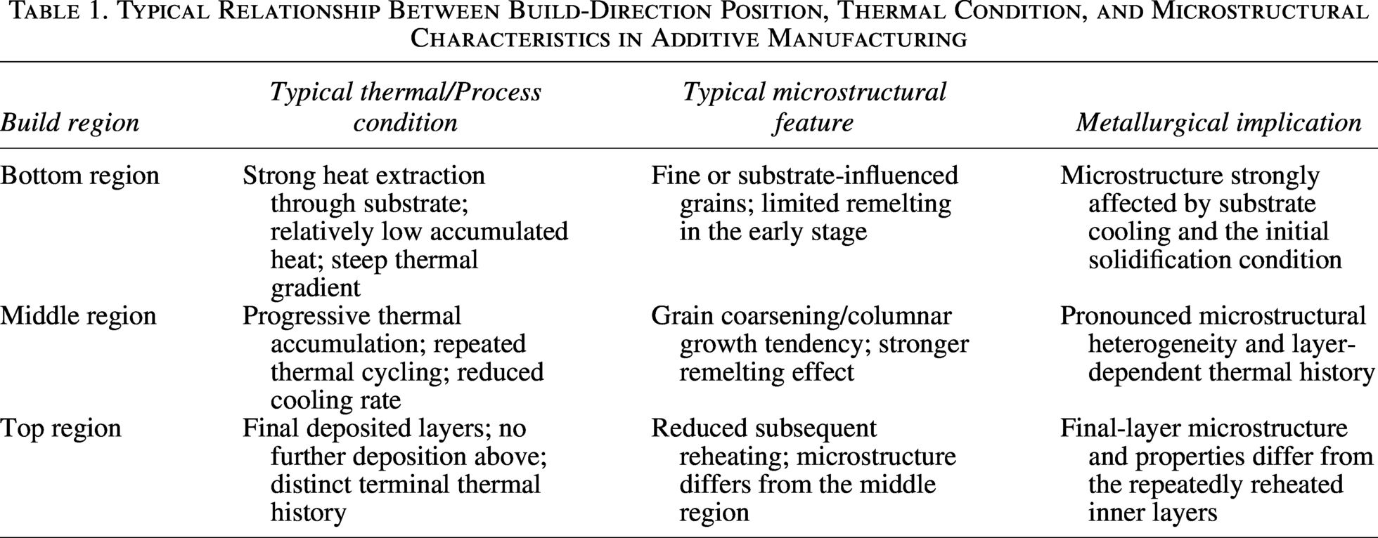
In AM, thermal accumulation generally increases with build height and leads to layer-dependent thermal histories.^14–16 As a result, the microstructure and related properties may vary along the build direction.^17–19 A commonly observed tendency is that the lower region of the build, which is strongly affected by heat extraction through the substrate, exhibits a relatively different solidification condition from the middle region, where repeated thermal cycling and thermal accumulation become more pronounced. In the upper region, the final deposited layers experience a distinct thermal history because no subsequent layers are deposited above them. These differences in thermal conditions can result in variations in grain morphology, remelting behavior, and microstructural heterogeneity along the build direction.^20–24 Such phenomena can be further understood from the perspectives of undercooling, nucleation, and thermal cycling.^25–29 For clarity, the typical relationship between build height, thermal condition, and microstructural distribution is summarized in Table 1. These build-direction-dependent thermal and microstructural variations indicate that heat input regulation is essential for improving melt pool consistency and reducing microstructural heterogeneity during WAAM.

Table 1.

Typical Relationship Between Build-Direction Position, Thermal Condition, and Microstructural Characteristics in Additive Manufacturing

Build region	Typical thermal/Process condition	Typical microstructural feature	Metallurgical implication
Bottom region	Strong heat extraction through substrate; relatively low accumulated heat; steep thermal gradient	Fine or substrate-influenced grains; limited remelting in the early stage	Microstructure strongly affected by substrate cooling and the initial solidification condition
Middle region	Progressive thermal accumulation; repeated thermal cycling; reduced cooling rate	Grain coarsening/columnar growth tendency; stronger remelting effect	Pronounced microstructural heterogeneity and layer-dependent thermal history
Top region	Final deposited layers; no further deposition above; distinct terminal thermal history	Reduced subsequent reheating; microstructure differs from the middle region	Final-layer microstructure and properties differ from the repeatedly reheated inner layers

The evolution of the melting pool depth can be well visualized by numerical methods with different kinds of heat source models.^30–34 The traditional heat source models like the Gaussian heat source model and double ellipsoid model used in welding simulations^35–37 can also be directly applied to AM for the temperature visualizations.^38–42 All temperature features, including maximum temperature rises, cooling rates, and the temperature gradients, can be well revealed by the numerical models.^43–45 In particular, particle features^46–48 and melt pool motions^49–51 can be further incorporated into the heat source model to highlight key features of AM. The details of temperature variations and thermal accumulations are well shown by numerical models. However, further work is needed to determine how to control thermal accumulation and ensure melt pool consistency along the build height.

Recent developments in artificial intelligence (AI) provide possible solutions to the challenges in AM. Xie et al.⁵² used a data-driven method to predict the melt pool geometries, in which simulation cases are used to form the database and Gaussian regression model is used to predict the keyhole sizes. Wang et al.⁵³ converted data like point clouds into control-field representations, and the map rules between control and property are set. Both the initial data and the mapping rules form the multi-information model to generate property data for industrial manufacturing. Mozaffar et al.⁵⁴ used neural networks for graph-based representation to obtain the thermal responses in AM, and the tests on directed energy deposition reveal the accuracy of the developed deep learning architecture on the prediction of thermal histories. Popova et al.⁵⁵ developed four-step data workflows to predict the process–structure relationships, in which data preprocessing, microstructure, dimensionality reduction, and extraction/validation are incorporated. The microstructures are predicted by the Potts Monte Carlo method, and the process parameters can be correlated with the final microstructures using the data-driven method. Herriott et al.⁵⁶ applied machine-learning and deep-learning methods to predict the microstructure-dependent mechanical properties of additively manufactured metals. Their study showed that AI-based models can effectively capture the relationship between microstructural features and mechanical properties, thereby demonstrating the potential of data-driven methods for process–microstructure–property analysis in AM. Xie et al.⁵⁷ used convolutional neural network integrating wavelet transforms to predict location-dependent mechanical properties based on the input temperature histories. The dominant mechanistic features like temperature ranges and thermal frequencies can be revealed by the developed data-driven computational framework. Nguyen et al.⁵⁸ presented a novel end-to-end AI-enhanced metal additive manufacturing lifecycle framework spanning the stages of design, build, post-processing, and end-of-life, which enables a more comprehensive evaluation of AI applications across the broader AM field. Representative applications of AI in AM are summarized in Table 2. Caggiano et al.⁵⁹ presented a process qualification-oriented, data-driven framework for WAAM, integrating qualification data, process monitoring, and feedback control. Xiong et al.⁶⁰ presented an adaptive control system for maintaining a constant distance between the nozzle and the top surface during GMAW-based layer AM. Love et al.⁶¹ developed a vision-based monitoring system integrated with a reinforcement learning framework to enable intelligent in situ monitoring and control of WAAM. Xia et al.⁶² proposed a deep-learning-based vision monitoring method for diagnosing different anomalies during the WAAM process. AI can be used to establish data-driven relationships between process parameters and process responses in AM.^63–67 In this work, AI is employed to predict the current required under different layer-number and layer-thickness conditions for improving melt pool depth consistency in WAAM. Accordingly, the present study focuses on an AI-assisted offline heat input design for improving melt pool depth consistency in WAAM.

Table 2.

Representative Applications of Artificial Intelligence in Additive Manufacturing

Reference	AI method	Objective category	Main task
Xie et al.⁵²	Gaussian regression/Data-driven model	Prediction	Prediction of keyhole/Melt-pool-related geometric features
Wang et al.⁵³	Field-driven data processing	Optimization/Property mapping	Mapping between control field and property field
Mozaffar et al.⁵⁴	Graph neural network	Prediction	Prediction of thermal histories
Popova et al.⁵⁵	Data science workflow	Process–structure mapping	Linking process parameters to microstructure
Herriott et al.⁵⁶	CNN + ridge regression	Prediction	Prediction of microstructure-dependent mechanical properties
Xie et al.⁵⁷	CNN + wavelet transforms	Prediction	Prediction of location-dependent mechanical properties from thermal histories
Nguyen et al.⁵⁸	Review/Lifecycle framework	Review/Framework	Lifecycle-level overview of AI in MAM

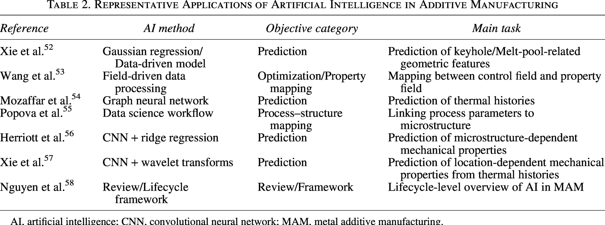
AI, artificial intelligence; CNN, convolutional neural network; MAM, metal additive manufacturing.

Recent studies have demonstrated the strong potential of AI in AM for applications such as prediction, monitoring, and process–structure/property mapping. However, comparatively fewer studies have focused on the layer-by-layer design of heat input for mitigating thermal accumulation and improving melt pool depth consistency during WAAM deposition. This gap is important because thermal accumulation along the build direction leads to layer-dependent thermal histories, melt pool variations, and microstructural heterogeneity, which in turn affect the quality and stability of deposited components. To address this issue, the present study develops an AI-assisted heat input design using a backpropagation neural network for the offline layer-by-layer design of heat input in WAAM. The specific objective is to establish the relationship among layer number, layer thickness, and the required current to maintain a more consistent melt pool depth under thermal accumulation conditions. In this way, the present work provides a focused step toward AI-assisted heat input regulation in WAAM while also offering a basis for future experimentally validated control strategies.

Models and Methods

Model description

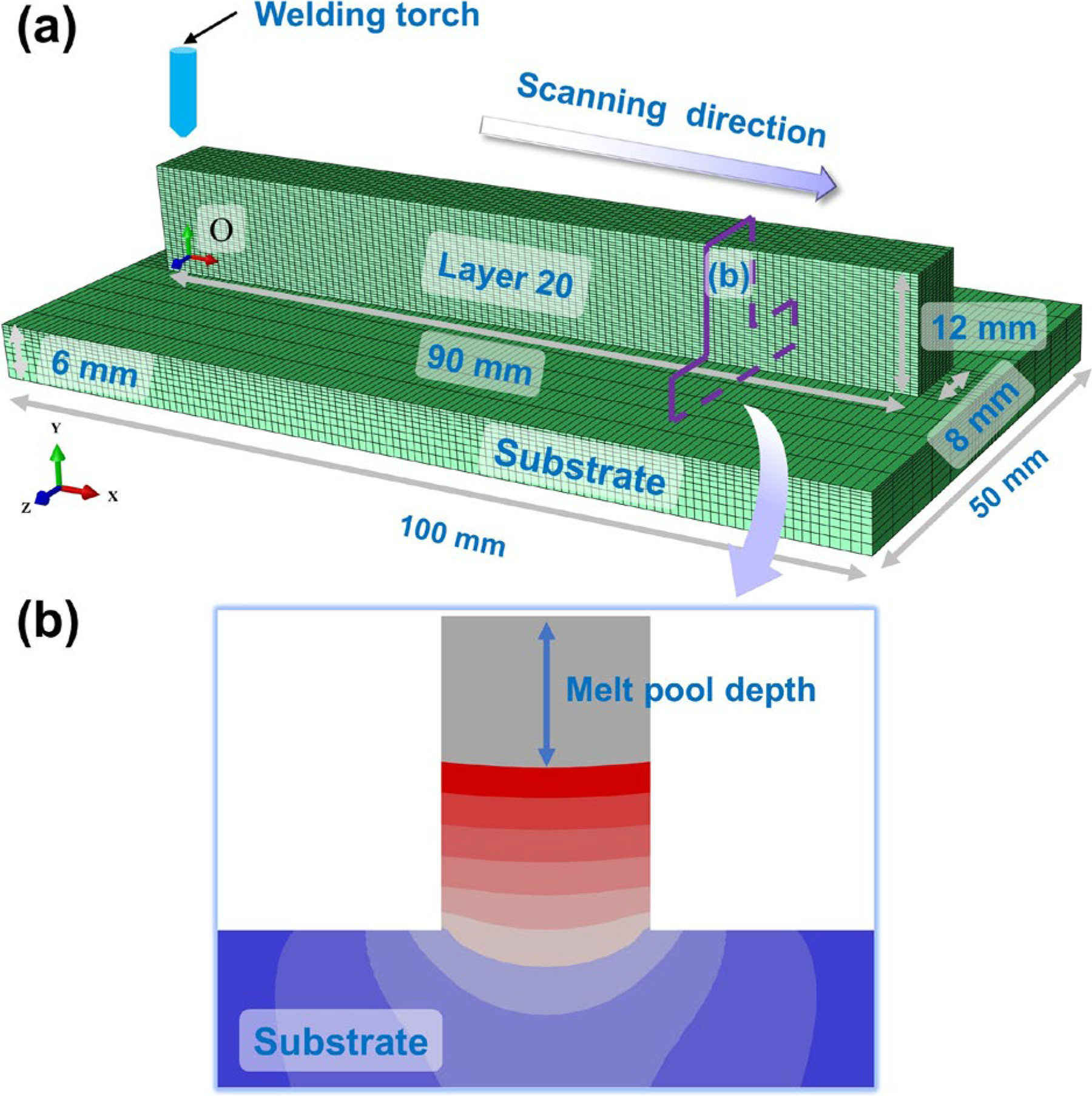
The finite element model is shown in Figure 1a. The substrate dimensions are 100 × 50 × 6 mm. The dimensions of the 20 deposited layers are 90 × 8 × 0.6 mm. The mesh is generated with linear hexahedral element DC3D8. The melt pool is shown in Figure 1b.

FIG. 1.

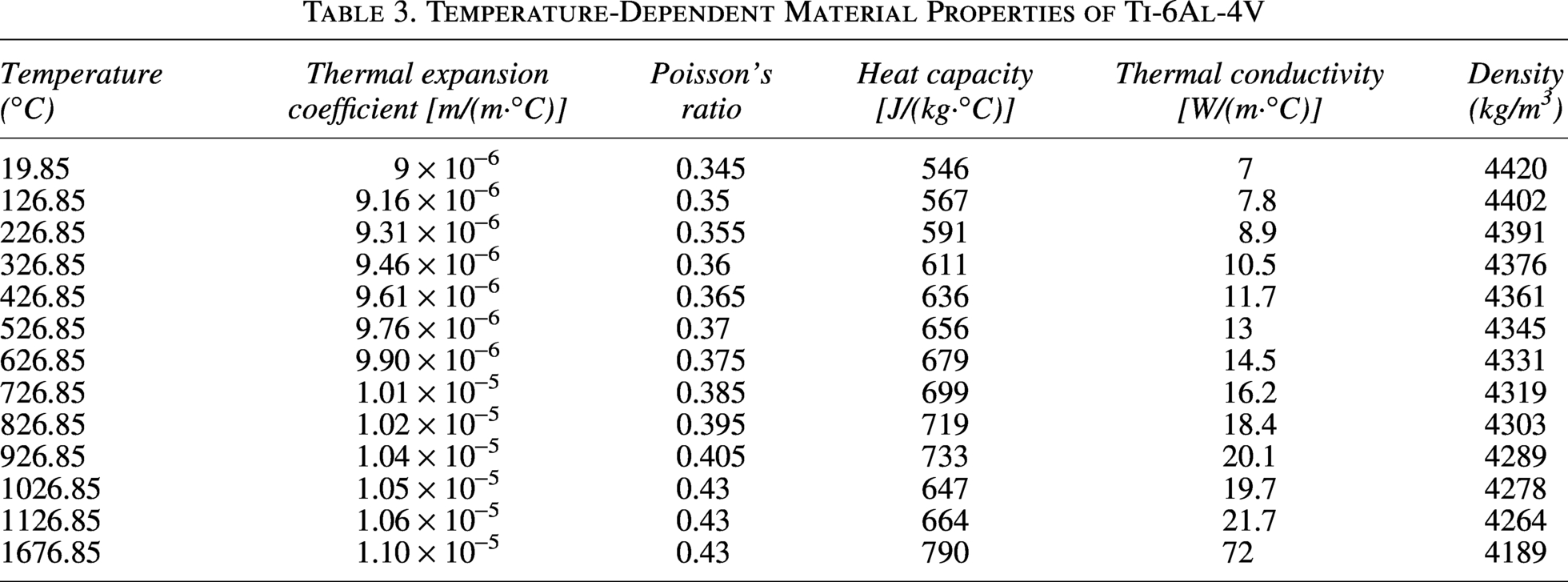
Numerical simulation: (a) finite element model and (b) melt pool.

Both the substrate and the deposited materials are Ti-6Al-4V. The temperature-dependent material properties of Ti-6Al-4V are listed in Table 3.⁶⁸ The mechanical properties of the deposited material are assumed to be identical to the substrate. The current is 180 A, the voltage is 15 V, and the scanning speed is 300 mm/min.

Table 3.

Temperature-Dependent Material Properties of Ti-6Al-4V

Temperature (°C)	Thermal expansion coefficient [m/(m·°C)]	Poisson’s ratio	Heat capacity [J/(kg·°C)]	Thermal conductivity [W/(m·°C)]	Density (kg/m³)
19.85	9 × 10⁻⁶	0.345	546	7	4420
126.85	9.16 × 10⁻⁶	0.35	567	7.8	4402
226.85	9.31 × 10⁻⁶	0.355	591	8.9	4391
326.85	9.46 × 10⁻⁶	0.36	611	10.5	4376
426.85	9.61 × 10⁻⁶	0.365	636	11.7	4361
526.85	9.76 × 10⁻⁶	0.37	656	13	4345
626.85	9.90 × 10⁻⁶	0.375	679	14.5	4331
726.85	1.01 × 10⁻⁵	0.385	699	16.2	4319
826.85	1.02 × 10⁻⁵	0.395	719	18.4	4303
926.85	1.04 × 10⁻⁵	0.405	733	20.1	4289
1026.85	1.05 × 10⁻⁵	0.43	647	19.7	4278
1126.85	1.06 × 10⁻⁵	0.43	664	21.7	4264
1676.85	1.10 × 10⁻⁵	0.43	790	72	4189

Heat transfer

The transient temperature field T(x, y, z, t) can be determined by the solution to the 3D heat conduction equation along with the relevant boundary conditions. The energy balance equation is as follows:

\frac{\partial}{\partial x} (k \frac{\partial T}{\partial x}) + \frac{\partial}{\partial y} (k \frac{\partial T}{\partial y}) + \frac{\partial}{\partial z} (k \frac{\partial T}{\partial z}) + Q = \frac{\partial (ρ C_{p} T)}{\partial t}

(1)

where t represents the time, C_p is the specific heat capacity, ρ is the density, T denotes temperature, k is the thermal conductivity, and Q is the power generated per unit volume within the workpiece. The coordinates x, y, and z define the coordinate system related to the heat source.

A double-ellipsoid heat source model is selected to simulate the heat input in this WAAM model. The power density in the front ellipsoid is given by the following equation:

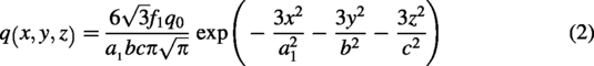
q (x, y, z) = \frac{6 \sqrt{3} f_{1} q_{0}}{a_{_{1}} b c π \sqrt{π}} \exp (- \frac{3 x^{2}}{a_{1}^{2}} - \frac{3 y^{2}}{b^{2}} - \frac{3 z^{2}}{c^{2}})

(2)

The power density in the rear ellipsoid is given by the following equation:

q (x, y, z) = \frac{6 \sqrt{3} f_{2} q_{0}}{a_{_{2}} b c π \sqrt{π}} \exp (- \frac{3 x^{2}}{a_{2}^{2}} - \frac{3 y^{2}}{b^{2}} - \frac{3 z^{2}}{c^{2}})

(3)

where f₁ = 0.7 and f₂ = 1.3 are thermal input parameters; a₁ = 0.004 m, a₂ = 0.006 m, b = 0.006 m, and c = 0.002 m are shape parameters; a₁ and a₂ determine the length of the ellipsoid in the front and rear sides of the double-ellipsoid heat source, respectively; and b and c determine the width and the depth of the double-ellipsoid heat source model, respectively. The initial values of the Goldak double-ellipsoidal heat source parameters were estimated using the geometry-based initialization rules proposed by Goldak.⁶⁹ In the present notation, b was initialized as one-half of the experimentally measured melt-pool width, c as the experimentally measured melt-pool depth, a₁ as one-half of the measured melt-pool width, and a₂ as twice the measured melt-pool width. These initial estimates were subsequently refined using the experimentally observed melt-pool cross-sections.⁷⁰ The schematic of the double-ellipsoid heat source model and the corresponding shape parameters are shown in Figure 2.

FIG. 2.

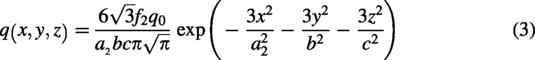
Double-ellipsoid heat source shape parameters.

Usually, the thermal input q₀ is constant during the AM process. But the temperature can be increased with the increase in building height due to thermal accumulations. To solve this problem, a BP neural network method is used to determine the layer-wise current required for heat input adjustment. The heat input is adjusted by changing the current for different deposited layers. In this way, the heat input can be varied by adjusting the layer-wise current. The heat input is determined by voltage, current, and thermal input efficiency.

q_{0} = η V I_{BP}

(4)

where η represents the efficiency, V stands for the voltage, and I_BP denotes the current calculated by the BP neural network.

The temperature field was not directly measured in the experiment. Instead, it was modeled using a 3D transient heat conduction model with a Goldak double-ellipsoidal heat source and temperature-dependent material properties. Accordingly, the present study uses indirect thermal validation through comparison of fusion-zone geometry and substrate penetration, rather than direct in situ temperature-field measurement.

For the deposition process, the elements assigned to the deposited layers were initially inactive and were activated sequentially along the prescribed scanning path as the moving heat source advanced. At each time increment, the volumetric heat input was applied only to the currently active elements, thereby ensuring a consistent coupling between material addition, heat input, and the layer-by-layer deposition sequence.^71,72

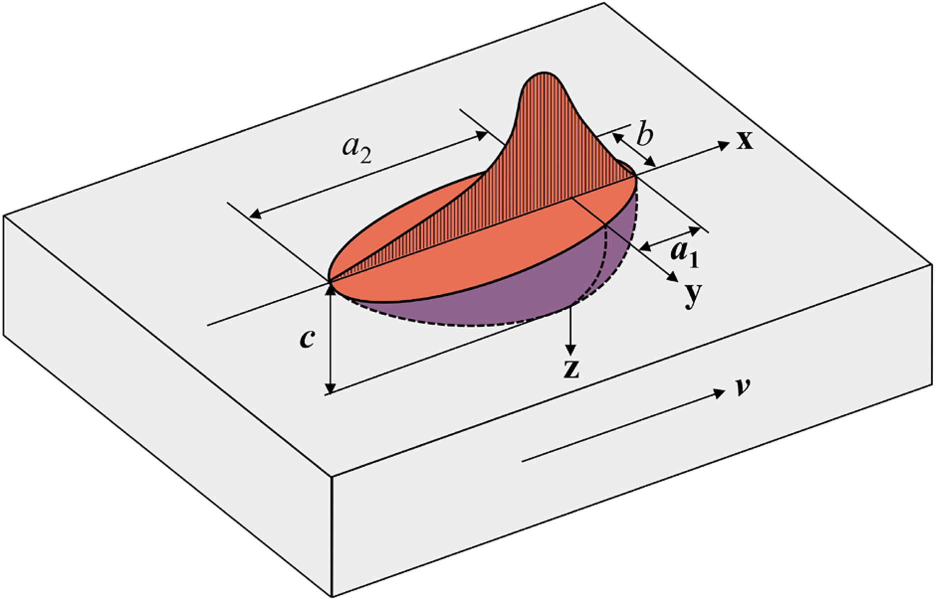
BP neural network

The BP network is a type of multilayer feedforward network with unidirectional propagation, with the backpropagation algorithm. The flowchart of the BP algorithm is shown in Figure 3a. It is composed of an input layer, a hidden layer, and an output layer, as illustrated in Figure 3b. The layer thickness (h) and the number of layers (n) are given as input parameters. The corresponding current (I) through each layer is selected to be the output parameter. The BP neural network was selected in this study as a practical nonlinear regression model. The mapping from layer number and layer thickness to the required current is highly nonlinear, particularly because of the sharp variation in the early layers and the gradual stabilization in the later layers. In such a case, polynomial fitting would require a predefined functional form, whereas the BP neural network can learn the nonlinear relationship directly from the dataset. Moreover, previous studies on AM have reported that neural-network-based models are effective for bead-geometry-related prediction and may outperform conventional regression-based models when the underlying process relationship is strongly nonlinear.^73–76 Therefore, the BP neural network was used here to construct the layer-by-layer current prediction model.

FIG. 3.

BP neural network: (a) flowchart of the BP algorithm and (b) architecture of the BP neural network.

The core training process of the BP neural network is divided into two stages: forward propagation and backward propagation. In forward propagation, the input data are processed layer by layer through the network’s weights, the bias calculations, and the activation functions to generate the necessary output data. In backward propagation, the error between the predicted value and target values is propagated backward from the output layer to the input layer. The weights and the bias are then updated using the gradient descent method to optimize the network parameters, reducing the error.

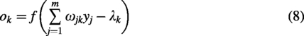
The neural network structure consists of an input layer, a hidden layer, and an output layer. In this model, h = (h₁, h₂, …, h_n) and n = (n₁, n₂, …, n_n) are considered to be the input data. I = (I₁, I₂, …, I_n₎ represents the data from the output layer. The parameter θ represents the weight vector connecting the input layer to the hidden layer. θ_ij represents the weight connecting the i-th input node to the j-th hidden layer node. λ represents the weight vector connecting the hidden layer to the output layer, specifically corresponding to the weight coefficients from the hidden layer nodes to the output layer nodes. The number of neurons in the hidden layer is 3. For instance, λ_jk represents the weight connecting the j-th hidden layer node to the k-th output layer node.

y_{i} = f (\sum_{i = 1}^{n} ω_{i j} x_{i} - θ_{j})

(5)

where ω_ij denotes the weight coefficient connecting the input to the output values. θ_j denotes the threshold for the signal from the input layer to the j-th node in the hidden layer.

y_{i} = f (n e t_{i})

(6)

n e t_{i} = \sum_{i = 1}^{n} ω_{i j} x_{i} - θ_{j}

(7)

where net_i represents the neural network structure formed by the i-th input node.

The computed output of the output nodes is given by,

o_{k} = f (\sum_{j = 1}^{m} ω_{j k} y_{j} - λ_{k})

(8)

where λ_k represents the threshold for the signal from the hidden layer to the k-th output node.

o_{k} = f (n e t_{j})

(9)

n e t_{j} = \sum_{j = 1}^{m} ω_{j k} y_{j} - λ_{k}

(10)

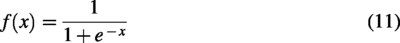
The function f in the above equation is the activation function being selected to be the form below:

f (x) = \frac{1}{1 + e^{- x}}

(11)

The error E is generated and needs to be updated in the backward propagation:

E = \frac{1}{2} {(d - o)}^{2}

(12)

where o is the output data, and d is the expected output data.

Deposition process

Ti-6Al-4V is used as both the deposited material and the substrate material. The experiments were carried out using a common MIG welder. The wire diameter is 1.2 mm, with a wire feeding rate of 1 m/min. The scanning speed is set to 300 mm/min, and the welding current is maintained at 180 A. The welding current was directly prescribed in the WAAM system during deposition. In contrast, the arc voltage was not directly recorded in the experiment. Therefore, a constant nominal voltage was adopted as the model input for heat input calculation. The adopted value was selected to be consistent with comparable Ti-6Al-4V WAAM conditions reported in the literature, where average arc voltages of ∼15 V.⁷⁷ The efficiency η is assumed to be 0.6. The experiments were performed under continuous deposition conditions. The interval between adjacent layers was short, and no intentional interlayer cooling was applied during the build. The ambient temperature was set to 25°C, and the convection coefficient was taken as 20 W/(m²·K). The substrate dimensions are 200 × 100 × 6 mm. 1-layer, 3-layer, and 5-layer specimens are fabricated on the substrate, as illustrated in Figure 4a and b. The 1-layer specimen is measured approximately to be 80 mm in length, 8 mm in width, and 0.6 mm in height. The 3-layer specimen is 80 × 8 × 1.8 mm, while the 5-layer specimen is 90 × 8 × 3 mm. The maximum width and the total deposited height of the additively manufactured wall were measured from the deposited geometry. In the numerical model, the deposition domain was constructed according to the measured maximum width and total height. For simplification, a uniform layer width was assumed for all deposited layers, and the layer height for each activated layer was taken as the total deposited height divided by the number of deposited layers. The corresponding deposition elements were initially defined as inactive and were activated sequentially along the predefined scanning path during the transient analysis. The deposited layers are cut on the cross-section at a distance of 3 cm along the scanning direction to obtain the specimens, as shown in Figure 4c–e. The cross-sections of the specimens are subsequently grounded, polished, and etched.

FIG. 4.

Wire arc additive manufacturing: (a) 1-layer and 3-layer deposits, (b) 5-layer deposit, (c) 1-layer specimen, (d) 3-layer specimen, and (e) 5-layer specimen.

Results and Discussions

Experimental verification

The numerical and experimental results were correlated through the comparison of cross-sectional fusion-zone geometry and substrate penetration. Specifically, the experimentally measured and simulated substrate penetration values were compared for the 1-layer, 3-layer, and 5-layer specimens at the selected cross-section. The resulting mean absolute percentage error (MAPE) was used to quantify the agreement between the numerical model and the experimental observations.

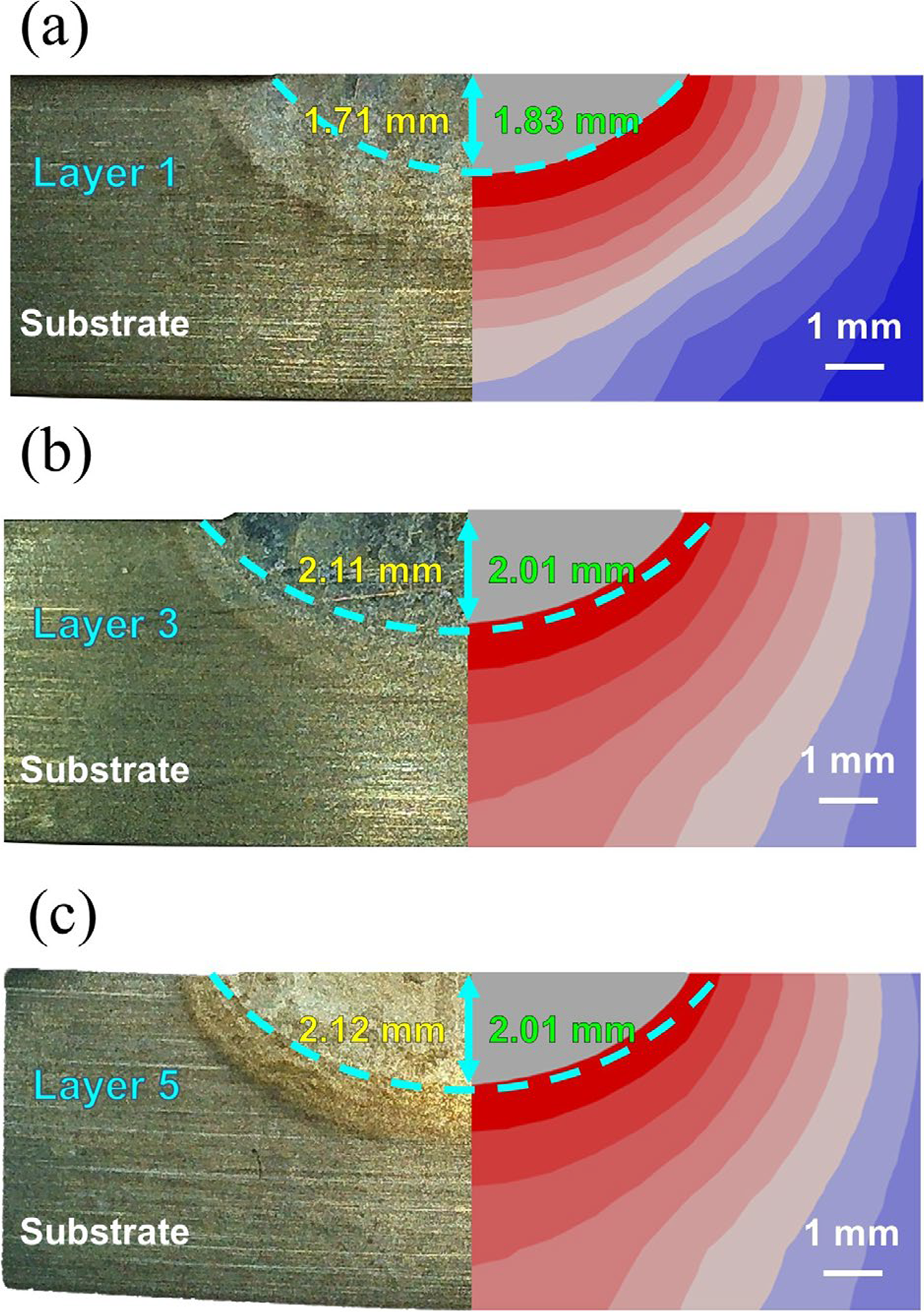
The cross-sections of the deposited specimens are shown in Figure 5. The overall fusion depths for the 1-layer, 3-layer, and 5-layer specimens are 2.26, 3.66, and 4.94 mm, respectively. The overall fusion depth increases with the number of deposited layers. The substrate penetrations are 1.71, 2.11, and 2.12 mm, respectively. The substrate penetration remains essentially unchanged between the 3-layer and 5-layer specimens.

FIG. 5.

Cross-sections of the experimental specimens: (a) 1-layer specimen, (b) 3-layer specimen, and (c) 5-layer specimen.

The numerical results on the cross-sections at different scan lengths (L_s) are shown in Figure 6. The melt pool in the simulation is determined according to the melting point of the deposited material, that is, 1660°C. At a scan length of 1 cm, the melt pool depths for the five layers are 2.34, 2.83, 3.17, 3.50, and 4.07 mm, respectively. When the scan length is increased to 5 cm, these values increase to 2.45, 3.25, 3.80, 4.17, and 4.47 mm. For substrate penetration, the values are 1.74, 1.63, 1.37, 1.10, and 1.07 mm at 1 cm, increasing to 1.85, 2.05, 2.00, 1.77, and 1.47 mm at 5 cm. Both the melt pool depth and the substrate penetration increase with increasing scan length.

FIG. 6.

Numerical simulation of cross-sections at different scan lengths: (a) layer 1, (b) layer 2, (c) layer 3, (d) layer 4, and (e) layer 5.

Figure 7 shows a comparison of substrate penetration between experimental and simulated results at a scan length of 3 cm. For layers 1, 3, and 5, the experimental values are 1.71, 2.11, and 2.12 mm, respectively, while the simulated values are 1.83, 2.01, and 2.01 mm. The MAPE of 5.65% indicates good agreement between the simulation and experimental results.

FIG. 7.

Comparison of substrate penetration between experimental and simulated results: (a) layer 1, (b) layer 3, and (c) layer 5.

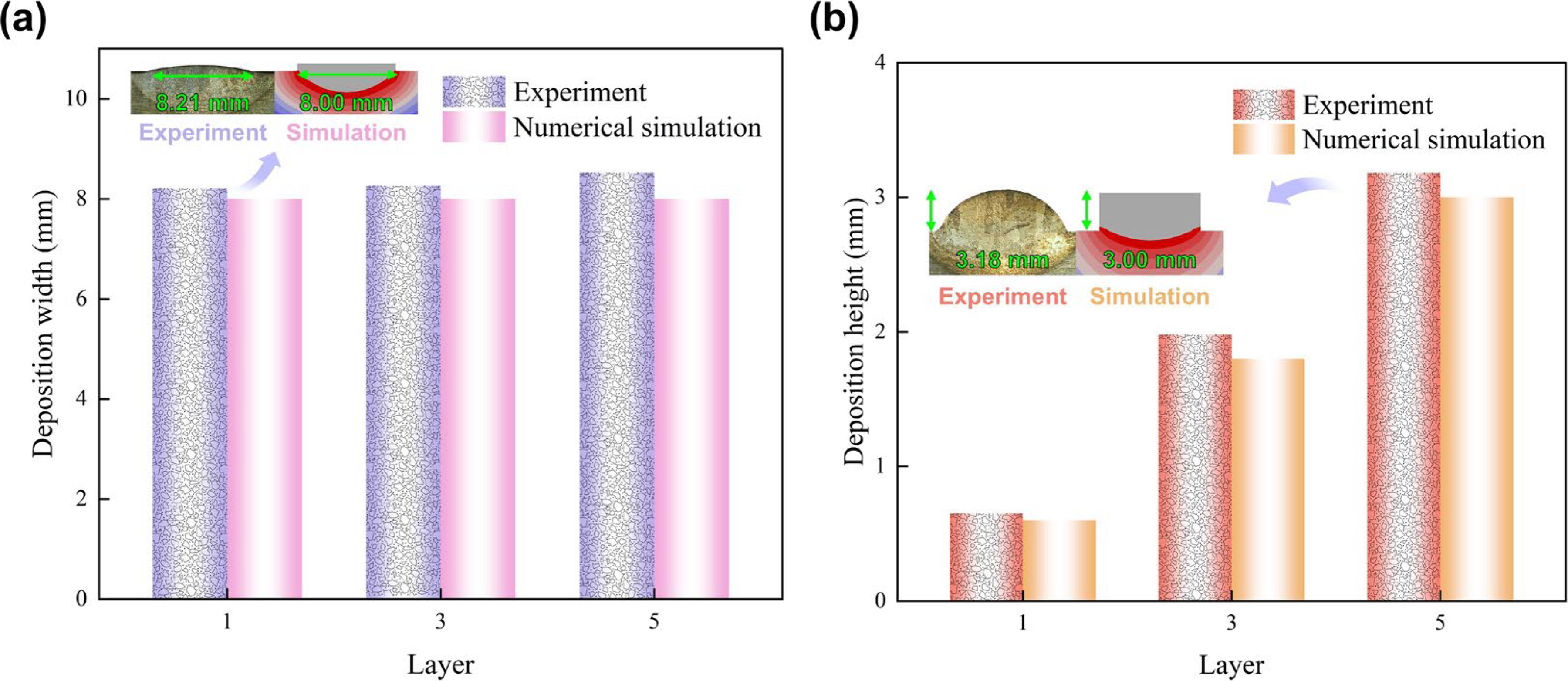
To verify the credibility of the numerical model, experimental measurements were compared with simulation results, as shown in Figure 8. In the experiments, the widths of layers 1, 3, and 5 range from 8.21 to 8.52 mm, while the simulated width is consistently 8 mm. The measured heights of layers 1, 3, and 5 are 0.65, 1.98, and 3.18 mm, respectively, whereas the corresponding simulated values are 0.6, 1.8, and 3.0 mm. The comparison shows that the MAPE for width and height is 3.94% and 7.48%, respectively.

FIG. 8.

Comparison between experiment and simulation: (a) deposition width and (b) deposition height.

Thermal accumulation under fixed heat input

Building upon the previous experimental cases, the numerical analysis was extended to a 20-layer simulation case to investigate the cumulative effect of thermal accumulation at a larger build height. Similar approaches have been used in previous WAAM simulation studies, where models validated on simpler experimental cases were further applied to analyze multilayer builds beyond the experimentally tested layer numbers.^78,79

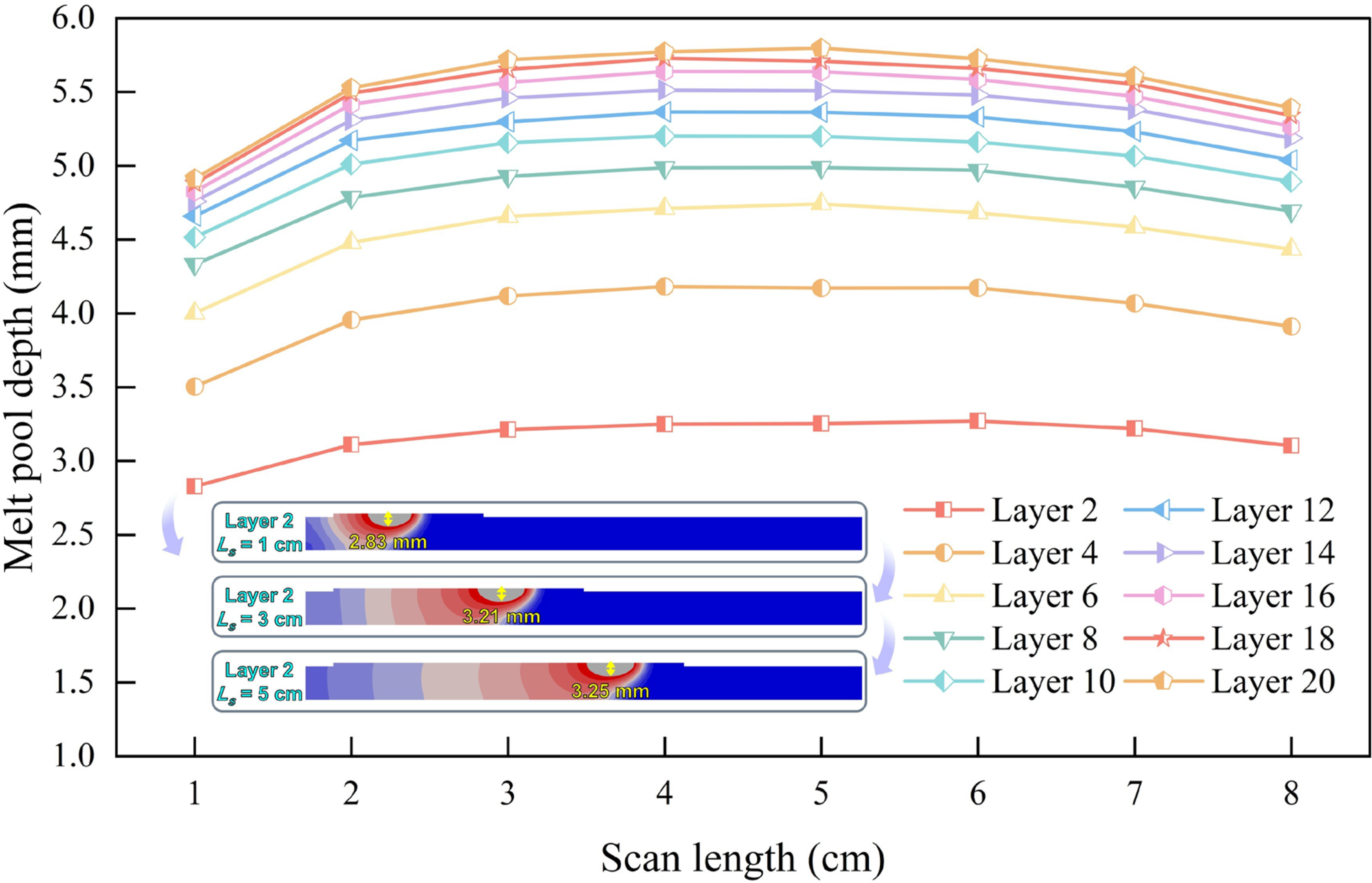
Figure 9 shows the melt pool depth evolution along the scanning path within a layer. When the scan length increases from 1 to 2 cm, the melt pool depth of layer 2 increases from 2.83 to 3.11 mm, representing a 9.89% increase. The melt pool depth of layer 4 increases from 3.50 to 3.96 mm, with a 13.14% increase. Layer 20 exhibits an increase from 4.91 to 5.53 mm, corresponding to a 12.63% increase. When the scan length increases from 2 to 8 cm, the melt pool depth of layer 2 changes by 0.17 mm (5.48), that of layer 4 changes by 0.27 mm (6.90%), and that of layer 20 changes by 0.40 mm (7.42%). From 1 to 2 cm along the scanning path, the melt pool depth increases noticeably. This indicates that the local thermal state is still evolving in the early stage of deposition, because the material at these positions has experienced different elapsed deposition times and different degrees of prior thermal accumulation. In contrast, from 2 to 8 cm, the variation in melt pool depth becomes much smaller, suggesting that the local thermal state along the scanning path has approached a relatively stable condition. Therefore, the melt pool depth at the midpoint of the scan path (4.5 cm) is selected as the representative value for each layer.

FIG. 9.

Melt pool depth evolution along the scanning path within a layer.

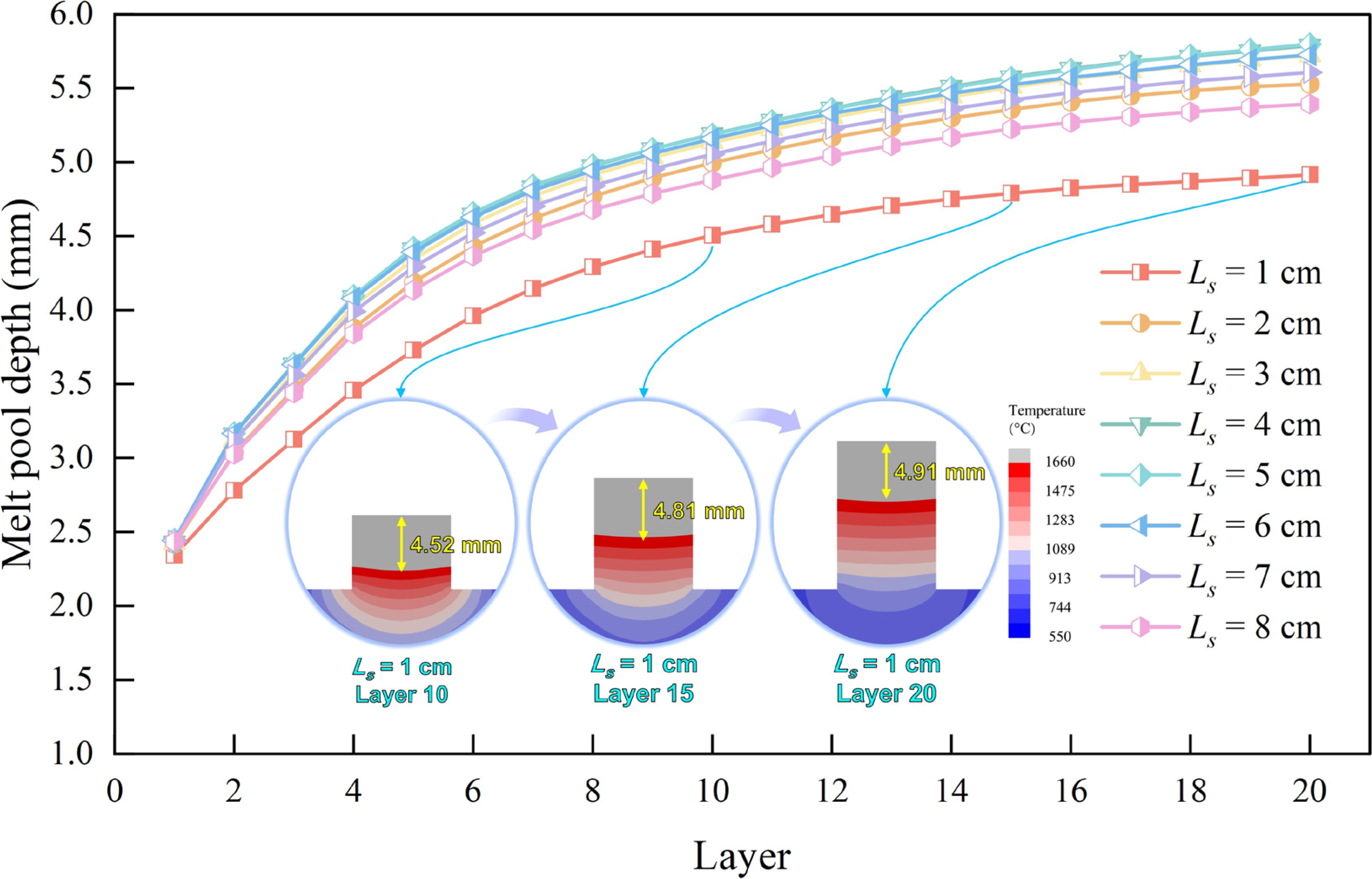
Figure 10 shows the melt pool depth evolution with increasing layer number. When the layer number increases from 1 to 2, the melt pool depth at a scan length of 1 cm increases from 2.34 to 2.83 mm, representing a 20.94% increase. At a scan length of 2 cm, the melt pool depth increases from 2.42 to 3.11 mm, with a 28.51% increase. At a scan length of 8 cm, the melt pool depth increases from 2.43 to 3.10 mm, corresponding to a 27.57% increase. When the layer number increases from 19 to 20, the melt pool depth at a scan length of 1 cm increases from 4.88 to 4.91 mm, with an increase of 0.61%. At a scan length of 2 cm, the melt pool depth increases from 5.51 to 5.53 mm, representing a 0.36% increase. At a scan length of 8 cm, the melt pool depth increases from 5.38 to 5.39 mm, with an increase of 0.19%. Thermal accumulation is relatively weak at a scan length of 1 cm. With the increase in the layer number, the melt pool depth still increases, but the increase rate slows down, indicating progressively weaker thermal accumulation effects.

FIG. 10.

Melt pool depth evolution with increasing layer number.

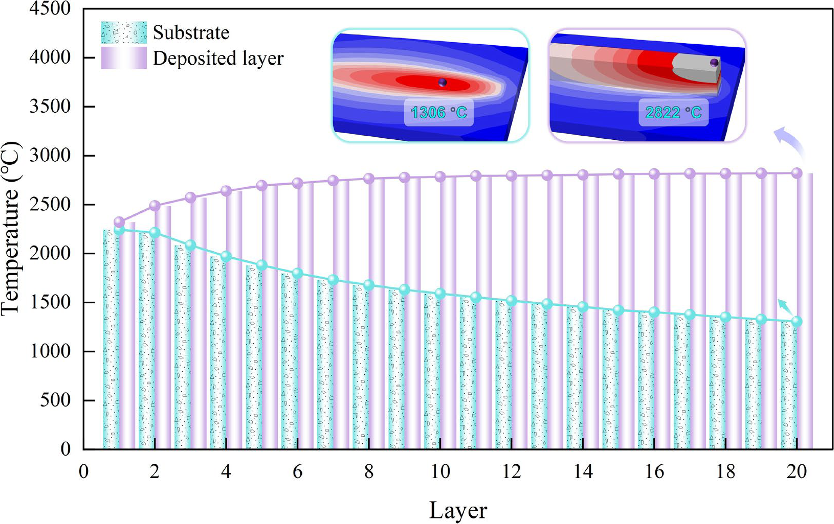
Figure 11 shows the variation in the maximum temperatures of the substrate and the deposited layers with increasing layer number. For layer 1, the local peak temperature of the substrate-side elements adjacent to the fusion boundary reaches 2244°C. As the layer number increases, the local peak value decreases, reaching 1306°C at layer 20. It should be noted that these values represent model-predicted transient local peaks near the fusion region, rather than the average temperature of the substrate or the interpass temperature. The simulation was carried out under a continuous-deposition condition without active interlayer cooling, which promotes stronger heat accumulation and repeated reheating during the build.^80–83 In contrast, for layer 1, the maximum temperature of the deposited layer is 2321°C. For layer 2, the maximum temperature of the deposited layer rises to 2488°C, representing a 7.20% increase. For layer 19, the maximum temperature of the deposited layer reaches 2820°C. For layer 20, it further rises to 2822°C, with a 0.07% increase. Heat accumulates in the deposited layer,^84–86 causing the maximum temperature to increase with the layer number, but the rate of increase slows down.

FIG. 11.

Variation in the maximum temperatures of the substrate and deposited layers with increasing layer number.

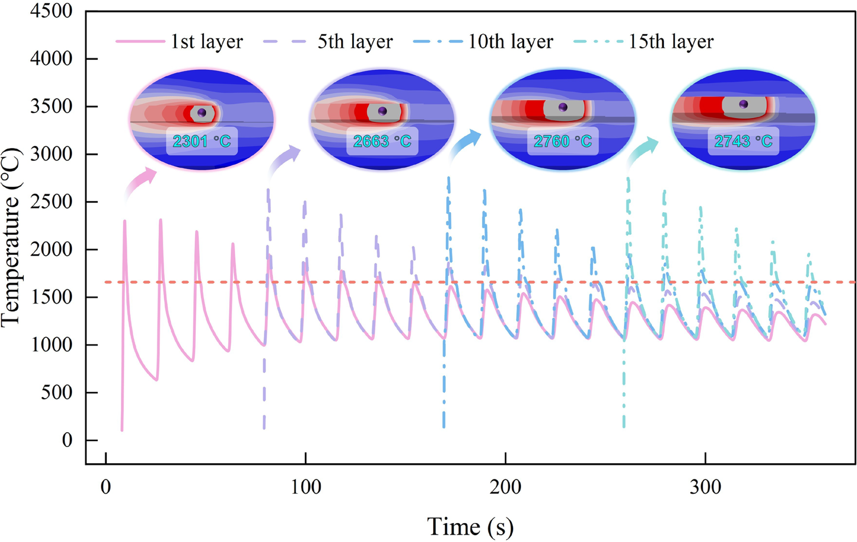
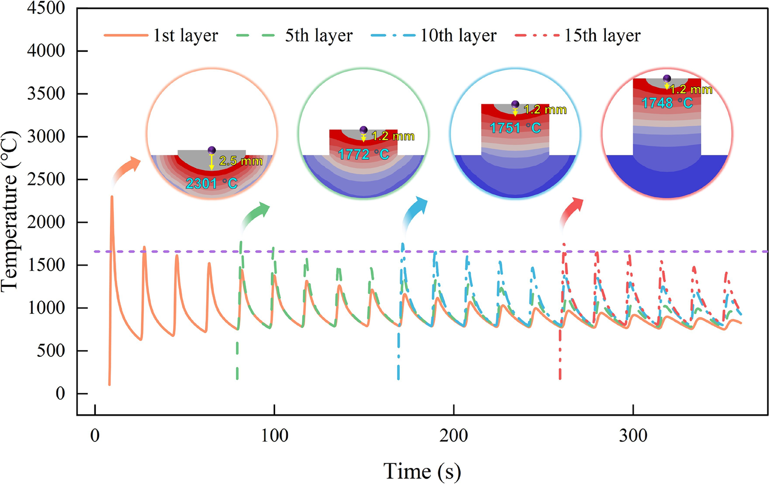
The temperature cycles extracted at a fixed point located at the midpoint of the scanning path on the top surface of layers 1, 5, 10, and 15 are shown in Figure 12. For layer 1, the temperature reaches 2301°C during its deposition. Owing to subsequent thermal accumulation, the temperature further increases to 2313°C during the deposition of layer 2 and then decreases. Layer 1 undergoes eight remelting cycles. For layer 5, the temperature reaches the maximum of 2663°C during its deposition and subsequently decreases. Layer 5 undergoes nine remelting cycles. Layers 10 and 15 reach their peak temperatures during their respective depositions, at 2760°C and 2790°C. Layer 10 undergoes nine remelting cycles. Since a total of 20 layers are deposited, the number of remelting cycles decreases for higher layers. Layer 15 undergoes five remelting cycles. Variations in the thermal cycles across different layers result in different melt pool depths. These variations lead to differences in grain morphology from layer to layer, which ultimately influences the mechanical properties. Therefore, controlling the melt pool depth of each layer is essential.

FIG. 12.

Temperature cycles of different layers.

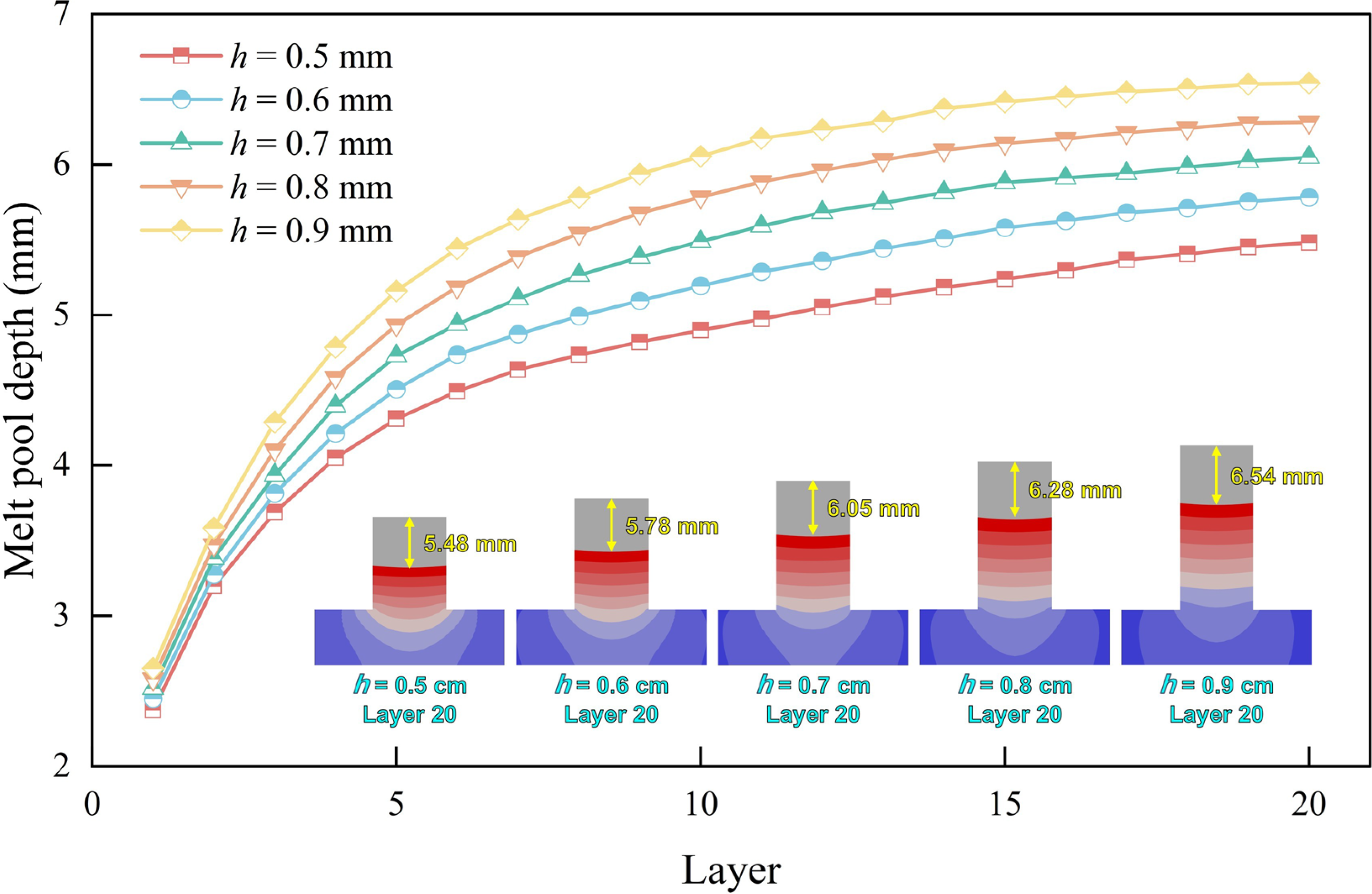
The melt pool depth for different deposited layer thicknesses is shown in Figure 13. For layer thicknesses of 0.5, 0.6, 0.7, 0.8, and 0.9 mm, the melt pool depth increases from layer 1 to layer 2 by 0.82, 0.83, 0.86, 0.89, and 0.93 mm, respectively. In contrast, from layer 19 to layer 20, the corresponding increases are 0.03, 0.03, 0.03, 0.01, and 0.01 mm, respectively. The melt pool depth increases, but the rate of increase slows down. From layer 1 to layer 20, the melt pool depth increases by 3.11, 3.33, 3.53, 3.70, and 3.89 mm, respectively. With increasing layer thickness, the melt pool depth increases more significantly, suggesting enhanced thermal accumulation.

FIG. 13.

Melt pool depth for different layer thicknesses.

AI-assisted heat input design

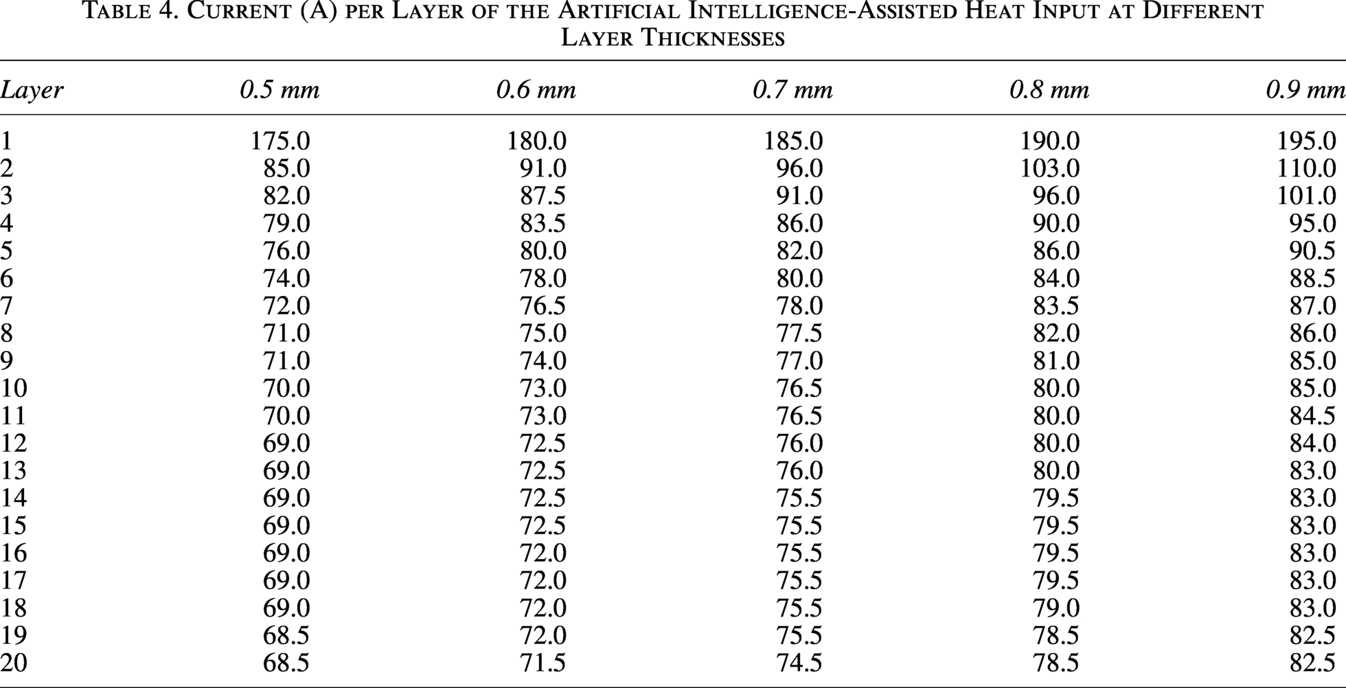
To maintain the melt pool depth across different layers within a relatively stable range, an AI-assisted heat input design is proposed. The AI-assisted heat input design is implemented through a layer-by-layer decreasing current strategy, in which the current is assigned individually to each layer to keep the melt pool depth at approximately twice the deposited layer thickness. For layer thicknesses ranging from 0.5 to 0.9 mm, the designed current values are summarized in Table 4 and used as the training set for the neural network. The neural network is used to establish the relationship among layer number, layer thickness, and the required current. The proposed method is an offline layer-by-layer heat input design based on the current adjustment. Given the layer number and layer thickness, the AI-assisted heat input design predicts the corresponding current values for the deposited layers.

Table 4.

Current (A) per Layer of the Artificial Intelligence-Assisted Heat Input at Different Layer Thicknesses

Layer	0.5 mm	0.6 mm	0.7 mm	0.8 mm	0.9 mm
1	175.0	180.0	185.0	190.0	195.0
2	85.0	91.0	96.0	103.0	110.0
3	82.0	87.5	91.0	96.0	101.0
4	79.0	83.5	86.0	90.0	95.0
5	76.0	80.0	82.0	86.0	90.5
6	74.0	78.0	80.0	84.0	88.5
7	72.0	76.5	78.0	83.5	87.0
8	71.0	75.0	77.5	82.0	86.0
9	71.0	74.0	77.0	81.0	85.0
10	70.0	73.0	76.5	80.0	85.0
11	70.0	73.0	76.5	80.0	84.5
12	69.0	72.5	76.0	80.0	84.0
13	69.0	72.5	76.0	80.0	83.0
14	69.0	72.5	75.5	79.5	83.0
15	69.0	72.5	75.5	79.5	83.0
16	69.0	72.0	75.5	79.5	83.0
17	69.0	72.0	75.5	79.5	83.0
18	69.0	72.0	75.5	79.0	83.0
19	68.5	72.0	75.5	78.5	82.5
20	68.5	71.5	74.5	78.5	82.5

Each combination of layer thickness and layer number corresponds to one current value, yielding a total of 100 samples. Among them, 70% is used as the training set, 15% as the validation set, and 15% as the test set. The layer thickness and layer number are input variables, while the current value is taken as the output. To improve the training performance, both input and output vectors are normalized prior to training. After normalization, the original data are transformed into dimensionless values ranging from −1 to 1, which can be expressed as:

T^{'} = 2 \frac{T - T_{min}}{T_{max} - T_{min}} - 1

(13)

L^{'} = 2 \frac{L - L_{min}}{L_{max} - L_{min}} - 1

(14)

I^{'} = 2 \frac{I - I_{min}}{I_{max} - I_{min}} - 1

(15)

where T′ and L′ are dimensionless input vectors used for training, and I′ is the output vector. T_min and L_min are the minimum input values, T_max and L_max are the maximum input values, I_min is the minimum output value, and I_max is the maximum output value. Once training is complete, the predicted values can be retrieved by reversing the normalization process.

To investigate whether the training set size is sufficient, the relative error (e) and correlation coefficient (ρ) between the true and identified current values for 10 different sizes (10%, 20%, 30%, 40%, 50%, 60%, 70%, 80%, 90%, and 100% of the total size) are analyzed. Training performance improves as ρ approaches 1 and e approaches 0.

Let I^t and Iⁱ represent the true and identified current values in the test set, respectively; the correlation coefficient ρ(I^t, Iⁱ) and relative error e(I^t, Iⁱ) can be described as:

ρ (I^{t}, I^{i}) = \frac{1}{k - 1} \sum_{k = 1}^{K} (\frac{I_{k}^{t} - μ_{I^{t}}}{σ_{I^{t}}}) (\frac{I_{k}^{i} - μ_{I^{i}}}{σ_{I^{i}}}) = \frac{cov (I^{t}, I^{i})}{σ_{I^{t}} σ_{I^{i}}}

(16)

e (I^{t}, I^{i}) = \frac{\sqrt{\sum_{k = 1}^{K} {| I_{k}^{t} - I_{k}^{i} |}^{2}}}{\sqrt{\sum_{k = 1}^{K} {| I_{k}^{t} |}^{2}}} = \frac{‖ I^{t} - I^{i} ‖}{‖ I^{t} ‖}

(17)

where

μ_{I^{t}}

is the mean of the true value,

μ_{I^{i}}

is the mean of the identified value,

σ_{I^{t}}

is the standard deviation of the true values,

σ_{I^{i}}

is the standard deviation of the identified values, and

cov (g)

is the covariance between the true and identified values.

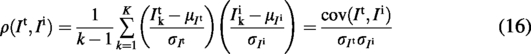
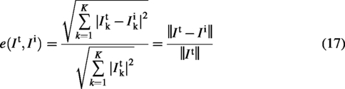
The correlation coefficients and relative errors for different training set sizes are shown in Figure 14. As the size of the training set increases, ρ gradually increases, while e correspondingly decreases. When the sample size exceeds 60, ρ stabilizes at approximately 0.997, approaching 1, and e stabilizes at about 0.026, approaching 0. Therefore, a dataset size of 100 is sufficient.

FIG. 14.

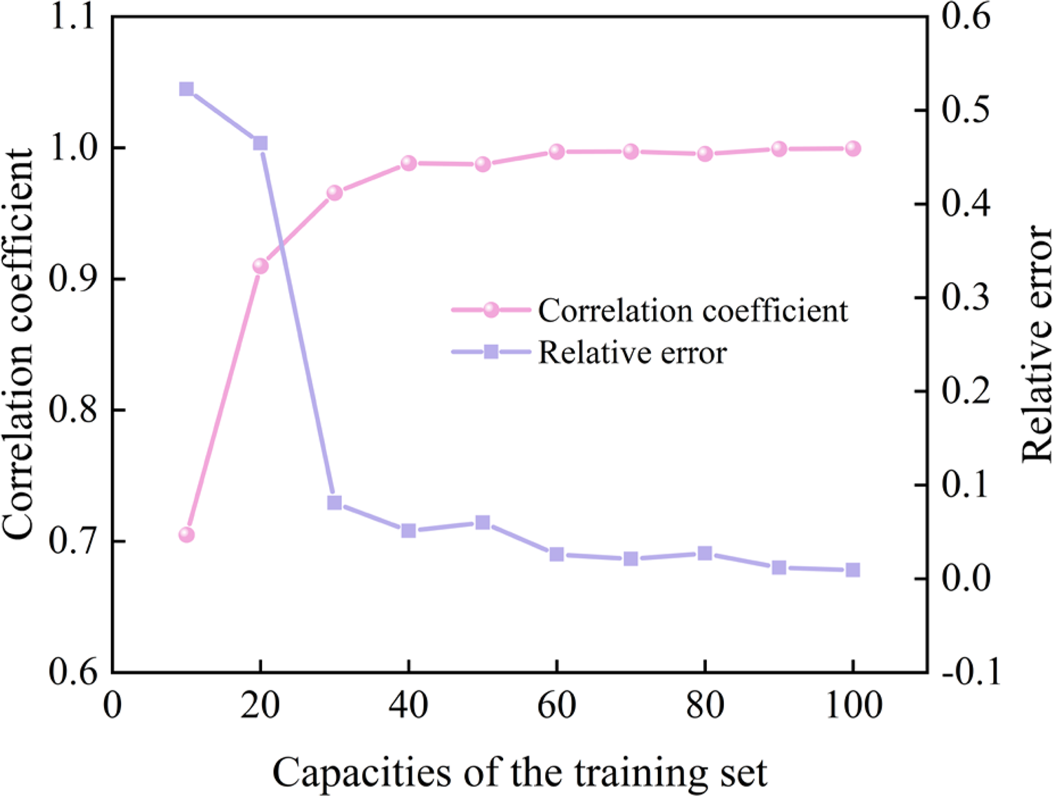
Correlation coefficient and relative error under different training set sizes.

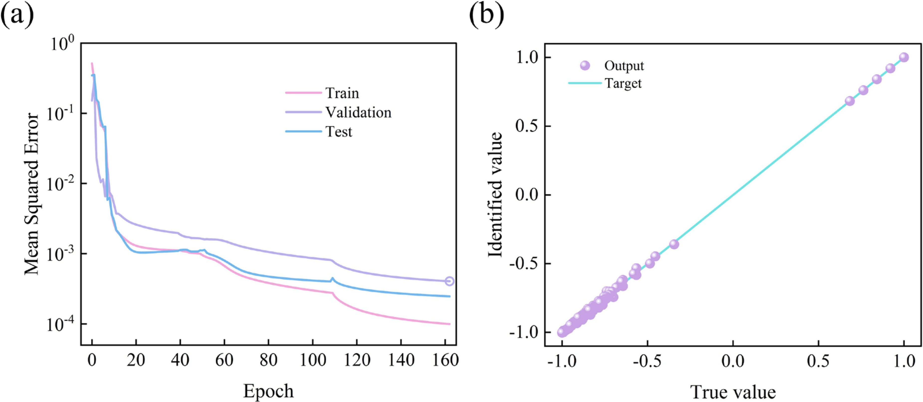
The error performance curve during training is shown in Figure 15a. The training process runs for a total of 162 epochs. As the number of epochs increases, the training, validation, and test errors all decrease. The best validation performance is achieved at the 162nd epoch, with a mean squared error of 4.06 × 10⁻⁴.

FIG. 15.

BP neural network: (a) training performance and (b) regression results.

The training regression results are shown in Figure 15b. The apparent two-region distribution in Figure 15 originates from the layer-dependent current values in the dataset. Specifically, under all five thickness conditions, the first layer requires a substantially higher current than the subsequent layers. Consequently, the first-layer samples are grouped in the high-current region, while the majority of the later-layer samples fall into the low-current region, which makes the intermediate region less populated. Most data points are close to the target line. The correlation coefficient between the predicted and actual values of the dataset is 0.99944, which is close to 1 and indicates a strong linear relationship. This demonstrates that the prediction model has good data fitting capability for the training samples and achieves satisfactory training performance.

Results under AI-assisted heat input

The temperature cycles of different layers under the AI-assisted heat input are shown in Figure 16. Compared with fixed heat input, the AI-assisted heat input reduces the peak temperatures for all layers. For layer 5, the maximum temperature is 1772°C, which is 891°C lower than that under fixed heat input, and the number of remelting cycles decreases from nine to one. For layer 10, the maximum temperature is 1751°C, representing a reduction of 1009°C, and the remelting cycles decrease from nine to one. For layer 15, the maximum temperature is 1748°C, which is 995°C lower, and the remelting cycles decrease from five to one. The use of the AI-assisted heat input effectively controls heat input and maintains consistency of melt pool depth across layers. The remelting behavior across layers becomes more uniform, reducing differences in thermal history. This homogenized thermal cycling strongly influences grain growth behavior and microstructural evolution, thereby improving microstructural uniformity and the stability of mechanical properties.

FIG. 16.

Temperature cycles of different layers using the artificial intelligence-assisted heat input at a layer thickness of 0.6 mm.

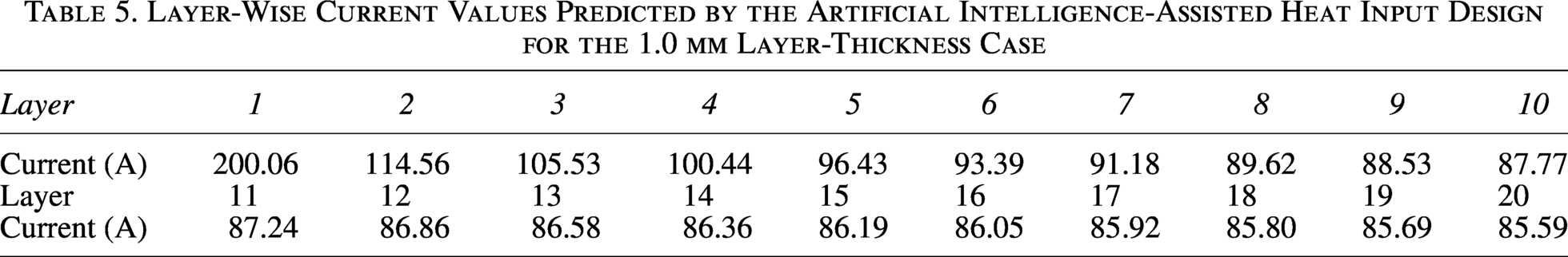
To further verify the feasibility of the prediction model, the AI-assisted heat input design was used to calculate the current values for a layer thickness of 1.0 mm. Layer-wise current values are listed in Table 5. The melt pool morphologies obtained using fixed heat input and AI-assisted heat input at a layer thickness of 1.0 mm are shown in Figure 17. The melt pool depth varies from 2.72 to 6.67 mm in traditional WAAM and can be adjusted to 1.92 to 2.72 mm using the proposed AI-assisted heat input design. Melt pool depth consistency is improved using the AI-assisted heat input design. The results show that the MAPE, mean absolute error, root mean square error, and coefficient of variation of the root mean square error are 2.8158%, 0.0563%, 0.0600%, and 3.0022%, respectively. These metrics describe the prediction error from the perspectives of relative deviation, average absolute deviation, overall error level, and normalized error dispersion, respectively, indicating the predictive accuracy of the proposed method.

Table 5.

Layer-Wise Current Values Predicted by the Artificial Intelligence-Assisted Heat Input Design for the 1.0 mm Layer-Thickness Case

Layer	1	2	3	4	5	6	7	8	9	10
Current (A)	200.06	114.56	105.53	100.44	96.43	93.39	91.18	89.62	88.53	87.77
Layer	11	12	13	14	15	16	17	18	19	20
Current (A)	87.24	86.86	86.58	86.36	86.19	86.05	85.92	85.80	85.69	85.59

FIG. 17.

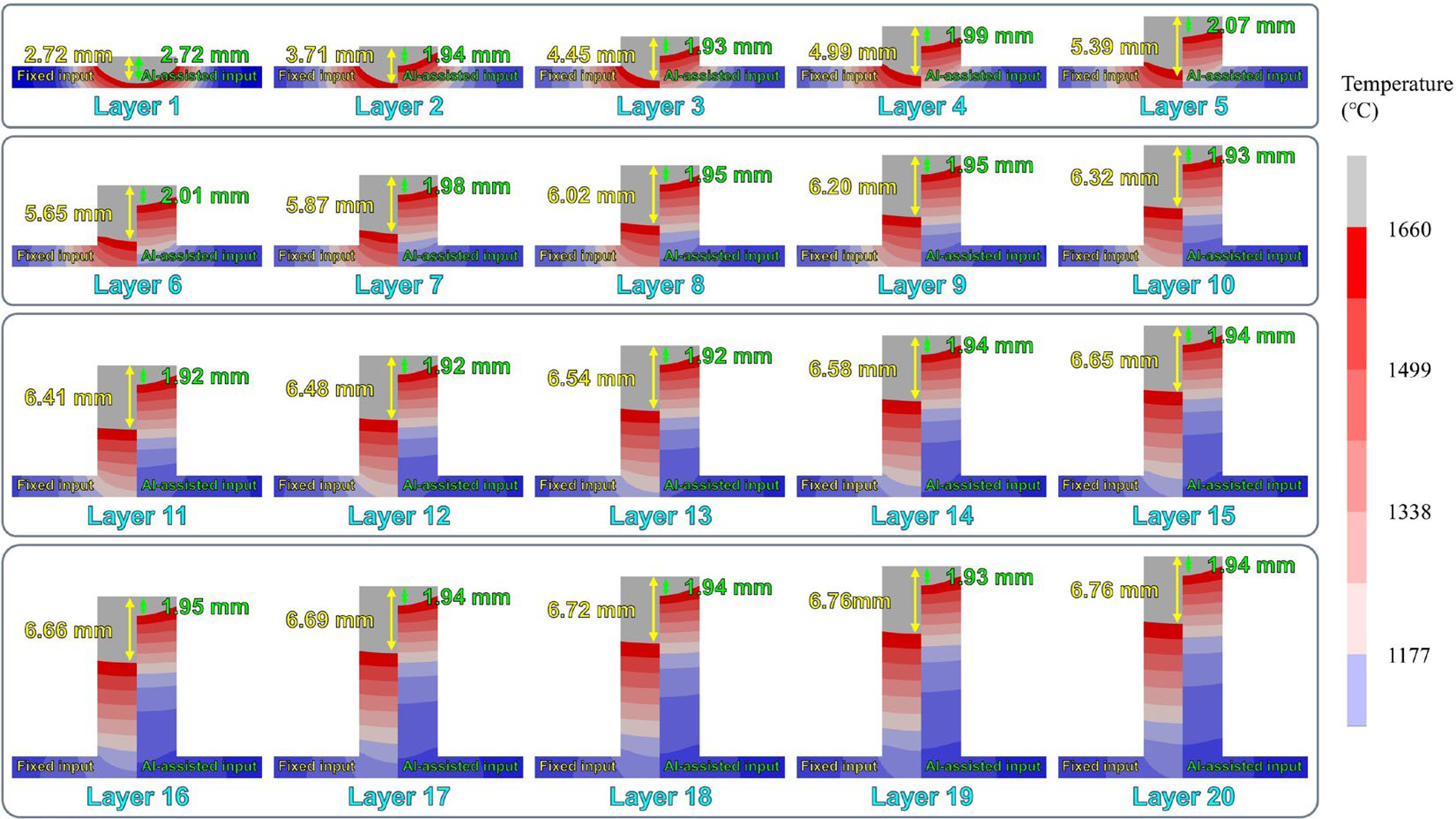
Melt pool morphologies using fixed heat input and artificial intelligence-assisted heat input.

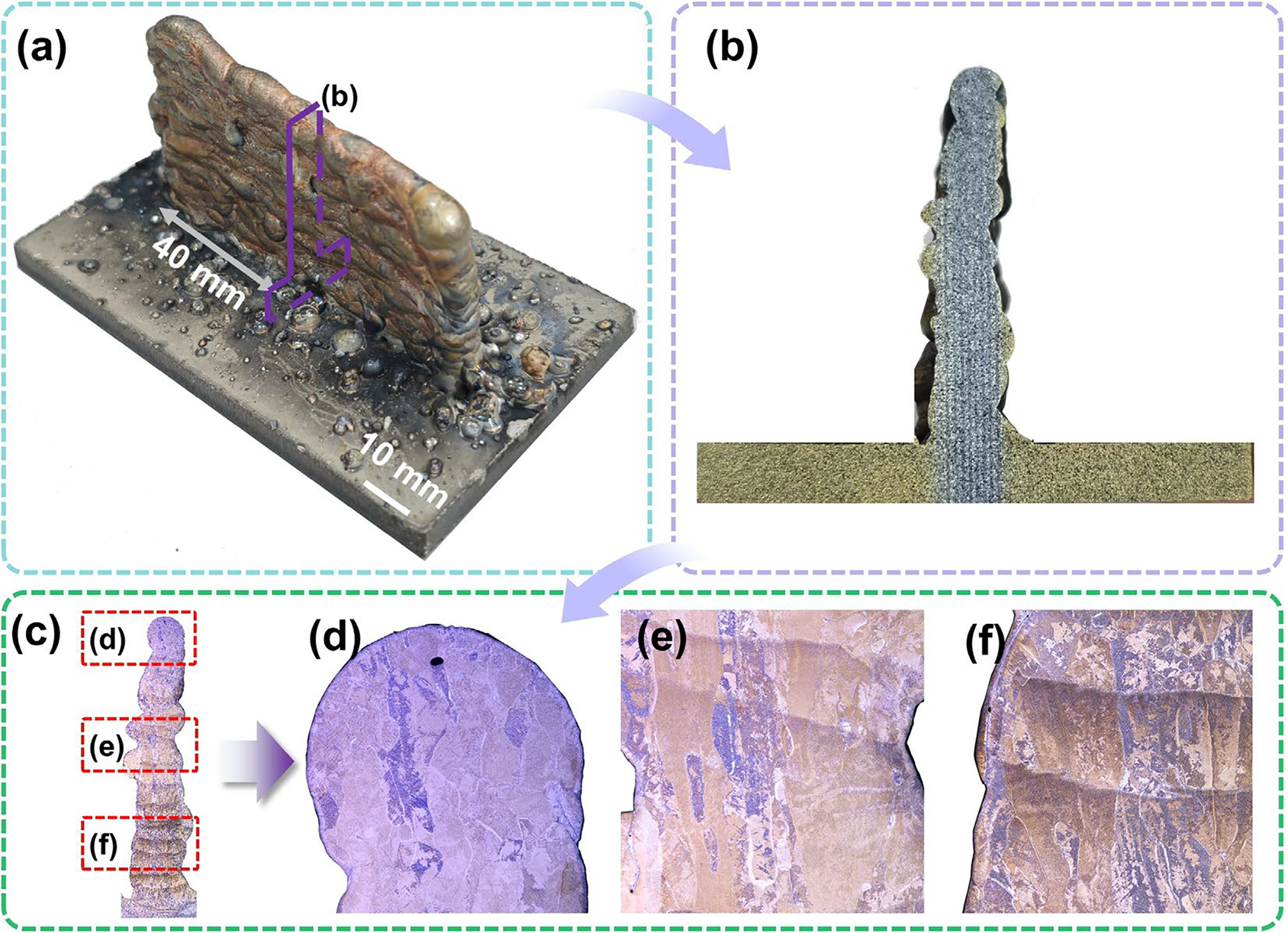
Additional experimental deposition was carried out to further examine the practical implementability of the layer-wise current schedule listed in Table 5, as shown in Figure 18. Figure 18a shows the 20-layer WAAM wall deposited using the AI-predicted layer-wise current schedule. The wall could be continuously formed without severe macroscopic collapse or discontinuity, indicating that the predicted current range was practically implementable under the present deposition conditions. Figure 18b shows the cross-section of the deposited wall, and Figure 18c presents the stitched metallographic cross-section. The cross-section shows a continuous deposited structure and metallurgical bonding between the deposited wall and the substrate. The enlarged regions in Figures 18d–f further show the local microstructural features at different build-height positions. It should be noted that the individual melt pool boundaries of each deposited layer cannot be clearly distinguished in the final cross-section, mainly because repeated remelting and thermal cycling during multilayer WAAM obscure the original layer-wise fusion boundaries. Therefore, this experiment is not used as a direct quantitative validation of transient layer-wise melt pool depth. Instead, it provides macro-forming and process-feasibility evidence for the AI-assisted heat input design.

FIG. 18.

Additional experimental deposition using the layer-wise current schedule listed in Table 5: (a) 20-layer deposited wall, (b) cross-section of the deposited wall, (c) metallographic cross-section, (d) metallography of the upper part of the cross-section, (e) metallography of the middle part of the cross-section, and (f) metallography of the lower part of the cross-section.

Limitations and future research

Although the proposed AI-assisted heat input design improves the simulated consistency of melt pool depth, some limitations should be noted. First, the present study still mainly relies on numerical simulation for evaluating the transient, layer-wise melt pool depth. The experimental results validate the thermal model indirectly through substrate penetration and deposited geometry, and the additional 20-layer deposition experiment in Figure 18 demonstrates the macro-forming feasibility of the AI-predicted layer-wise current schedule. However, the transient, layer-wise melt pool depth was not directly measured. Second, the thermal model includes several simplifications, such as constant nominal arc voltage, assumed heat input efficiency, simplified boundary conditions, and nominal layer geometry. These assumptions may affect the quantitative accuracy of the simulation under real WAAM conditions. Third, the proposed method is an offline heat input design method based on layer-wise current adjustment, not a real-time closed-loop control strategy. The predicted current schedule does not yet include feedback from melt pool geometry, arc signals, bead height, or interlayer temperature.

Future work will focus on direct experimental validation using in situ melt pool monitoring, thermal imaging, high-speed vision, or pyrometer-based temperature measurement. In addition, current adjustment should be combined with wire feed rate, travel speed, interlayer cooling, and bead-height monitoring to move toward closed-loop WAAM process control.

Conclusions

This study developed an AI-assisted heat input design using a BP neural network to improve the layer-to-layer consistency of melt pool depth in WAAM. The main findings are summarized as follows: 1.

Thermal accumulation becomes more pronounced with increasing build height in WAAM, resulting in layer-dependent thermal histories and an increase in melt pool depth under fixed heat input conditions.

A relationship among layer number, layer thickness, and the required current was established using a BP neural network, thereby enabling offline layer-by-layer heat input design for improving melt pool depth consistency.

For the additional validation case, the predicted melt pool depth showed an error of 2.82% relative to the target value, supporting the effectiveness of the proposed AI-assisted heat input design under simulated WAAM conditions.

The proposed AI-assisted heat input design improves melt pool depth consistency, narrowing the depth variation from 2.72–6.67 mm in traditional WAAM to 1.92–2.72 mm.

Authors’ Contributions

H.Z.: Writing—original draft, data curation, and formal analysis. Z.Z.: Writing—reviewing and editing, supervision, and project administration.

Data Availability Statement

The raw/processed data required to reproduce these findings cannot be shared at this time because of technical or time limitations but are available from the authors upon reasonable request.

Footnotes

Acknowledgments

The authors would like to acknowledge the help from Prof. Hongyang Wang at Dalian University of Technology with the experimental validation.

Author Disclosure Statement

The authors declare that they have no known competing financial interests or personal relationships that could have appeared to influence the work reported in this article.

Funding Information

This work was supported by the National Key Research and Development Program of China (2022YFB4600902) and the National Natural Science Foundation of China (12372191, 52332012).

References

1. Jia

, Yi

, Cao

, et al. Laser shock peening of TiC/inconel 625 composites fabricated via cored wire arc additive manufacturing. J Mater Process Technol 2026;348:119190.

2. Ramesh

, Gairola

, Jayaganthan

, et al. High-temperature tensile behaviour, fracture mechanism and constitutive modelling of additively manufactured AlSi9Cu3 alloy under varying strain rates. J Alloys Compd 2026;1056:186517.

3. Bhandari

, Vajpayee

, Da Silva

, et al. A review on additive manufacturing of piezoelectric ceramics: From feedstock development to properties of sintered parts. Mater Sci Eng R Rep. 2025;162:100877.

4. Sun

, Dong

, Liu

, et al. A critical review on additive manufacturing of continuous fiber-reinforced polymer composites: Materials, fabrication, structural design and novel functions. Thin-Walled Struct 2025;215:113491.

5. Noorbakhsh Nezhad

, Mohammadi Zahrani

, Mousavinasab

, et al. A comprehensive review of additively manufactured biomedical titanium alloys for bone tissue engineering: Biocorrosion, biomechanical, and biological properties. J Mater Res Technol 2025;36:9113–9157.

6. Li

, Wang

, Lindgren

L-E

, et al. Microstructure-based simulation of constitutive behaviors in friction stir additive manufacturing. Int J Mech Sci 2025;286:109863.

7. Zhang

. A review on additive manufacturing of wave controlling metamaterial. Int J Adv Manuf Technol 2023;124(3–4):647–680.

8. Nafis

, Whitt

, Iradukunda

A-C

, et al. Additive manufacturing for enhancing thermal dissipation in heat sink implementation: A review. Heat Transfer Eng 2021;42(12):967–984.

9. Yu

, France

, Du

, et al. Modeling of additively manufactured ceramic heat exchangers with semi-elliptical cross-section flow channels. Heat Transfer Eng 2025;46(11):909–918.

10.

10. Zarei

, Shabestari

, et al. Microstructural heterogeneity and anisotropic mechanical properties of titanium alloys manufactured by wire arc additive manufacturing: A review. J Mater Res Technol 2025;36:8381–8409.

11.

11. Omiyale

, Ogedengbe

, Ogbeyemi

, et al. Influence of heat input and uniform temperature distribution during wire arc additive manufacturing process: A critical review. Int J Adv Manuf Technol 2025;138(7–8):2673–2695.

12.

12. Mishra

, P. R

, Sajin Jose

, et al. Wire arc additive manufacturing: Materials, processes and its constraints. Mater Manuf Process 2025;40(6):723–740.

13.

13. Wu

, Pan

, Ding

, et al. A review of the wire arc additive manufacturing of metals: Properties, defects and quality improvement. J Manuf Process 2018;35:127–139.

14.

14. Wang

, Shi

, Fan

, et al. Role of process parameters on the elastocaloric effect of thin-walled NiTi shape memory alloys fabricated by additive manufacturing at the same energy density. J Manuf Process 2025;149:345–363.

15.

15. Yang

, Tang

, Li

, et al. Mitigating microstructural heterogeneity in laser-directed energy deposition Ni-based superalloys by heat accumulation in-situ heat treatment. Virtual Phys Prototyp 2025;20(1):e2509614.

16.

16. Huang

, Gu

, Liu

, et al. The effect of thermal history on elemental diffusion, phase evolution, and mechanical properties of laser powder bed fusion fabricated Ti6Al4V/AlMgScZr multi-material components. Addit Manuf 2025;107:104821.

17.

17. Negi

, Bairagi

, Arya

, et al. Microstructure, mechanical properties and phase transformation behaviour of directed energy deposition developed NiTixCu shape memory alloys. Mater Today Commun 2025;46:112953.

18.

18. Ziesing

, Berger

, Schaefer

, et al. From arc to alloy: Impact of directed energy deposition-arc/M on the microstructure and thermophysical properties of hot-work tool steels. J Mater Res Technol 2025;36:9662–9672.

19.

19. Zhang

, Zhou

, Chen

, et al. Numerical simulation for microstructure control in wire arc additive manufacturing of thin-walled structures. Thin-Walled Struct.2024;205:112581.

20.

20. Zeng

, Zhang

, Jin

, et al. Microstructure evolution and properties of inconel 625 alloy fabricated by hot-wire TIG additive manufacturing. J Alloys Compd 2025;1032:181113.

21.

21. Kim

, Kam

D-H

, Lee

K-A

. Characterization of the microstructure and mechanical properties of Ti-6Al-4V alloy fabricated by wire-arc additive manufacturing: Insights into fracture behavior and strengthening mechanism. Mater Sci Eng A 2025;939:148399.

22.

22. Zhang

, Zai

, Wang

, et al. Insight into microstructural evolution and mechanical property correlations of Ti2AlNb-based alloy fabricated through wire arc additive manufacturing. Mater Sci. Eng A 2025;938:148477.

23.

23. Feng

, Peng

, Huang

, et al. Enhancing strength-ductility synergy in wire arc additively manufactured CoCrNiTi medium-entropy alloys by adjusting Ni/Ti-rich precipitates. Mater Sci Eng. A 2025;941:148637.

24.

24. Sahoo

, Roy

. Novel insights on the microtexture formation in additive manufacturing of Ti-6Al-4V alloy. Mater Charact 2025;226:115159.

25.

25. Liu

, Wang

, Xiao

, et al. Insight into the mechanisms of columnar to equiaxed grain transition during metallic additive manufacturing. Addit Manuf 2019;26:22–29.

26.

26. Yao

, Gao

, Zhang

. Three-dimensional microstructure evolution of Ti–6Al–4V during multi-layer printing: A phase-field simulation. J Mater Res Technol 2022;20:934–949.

27.

27. Gao

, Yao

, Wang

, et al. Multiscale modeling of grain structure control in wire arc additive manufacturing of Ti6Al4V. J Mater Res Technol 2025;35:3980–3993.

28.

28. Xiong

, Lian

, Panwisawas

, et al. A microscale cellular automaton method for solid-state phase transformation of directed energy deposited Ti6Al4V. Addit Manuf 2024;95:104517.

29.

29. Liang

, Xue

, Yi

. Non-isothermal phase-field modeling and simulation of microstructure evolution in magnetic field-assisted selective laser sintering. Comput Methods Appl Mech Eng 2024;432:117387.

30.

30. Kundakcioglu

, Lazoglu

, Rawal

. Transient thermal modeling of laser-based additive manufacturing for 3D freeform structures. Int J Adv Manuf Technol 2016;85(1–4):493–501.

31.

31. Liu

, Liu

, Long

, et al. Influence of oscillating laser on forming characteristics and molten pool flow behavior of aluminum alloy double-wire additive manufacturing. J Laser Appl 2023;35(2):e022016.

32.

32. Chen

, Xue

, Zhong

, et al. AM-FEMU: An optimization method for additive manufacturing simulation parameters based on finite element model updating, utilizing three-dimensional deformation and melt pool temperature fields. Thin-Walled Struct 2025;209:112962.

33.

33. Beghini

, Stender

, Moser

, et al. A coupled fluid-mechanical workflow to simulate the directed energy deposition additive manufacturing process. Comput Mech 2021;67(4):1041–1057.

34.

34. Zhang

, Ge

, Li

, et al. Electromagnetic wave-based analysis of laser–particle interactions in directed energy deposition additive manufacturing. Addit Manuf 2020;34:101284.

35.

35. Aslam

, Sahoo

. Finite element analysis and experimental investigation of moving heat source model for GMAW deposited mild steel weld bead. Proc Inst Mech Eng E J Process Mech Eng. 2022;236(5):2218–2228.

36.

36. Friedrich

, Choo

. Thermal-stress characteristics of a large area additive manufacturing. Heat Transfer Eng 2023;44(13):1083–1098.

37.

37. Zhang

, Zhang

, Liu

, et al. The interface reaction and microstructure control in friction stir lap welding of Al and Ti dissimilar alloys. J Mater Res Technol 2025;35:6700–6714.

38.

38. Jiang

, Man

, Guo

, et al. Determination of residual stress field in laser cladding using finite element updating method driven by contour deformation. Opt Laser Technol 2024;179:111371.

39.

39. Prajadhiana

, Taufek

, Wan Abdul Rahaman

, et al. Distortion analysis method for wire arc additive manufacturing component using thermomechanical computation with enhanced separation and deposition algorithm. 3D Print Addit Manuf 2024;11(4):e1616–e1628.

40.

40. Ke

, Oliveira

, Cong

, et al. Multi-layer deposition mechanism in ultra high-frequency pulsed Wire Arc Additive Manufacturing (WAAM) of NiTi shape memory alloys. Addit Manuf 2022;50:102513.

41.

41. Cheng

, Huo

, Fernandez-Zelaia

, et al. A Gaussian process-based extended Goldak heat source model for finite element simulation of laser powder bed fusion additive manufacturing process. Comput Mater Sci 2024;244:113185.

42.

42. Zhang

, Tan

, Yao

, et al. Numerical methods for microstructural evolutions in laser additive manufacturing. Comput Math Appl 2019;78(7):2296–2307.

43.

43. Çalışkan

Cİ

, Koca

, Özer

, et al. Efficiency comparison of conformal cooling channels produced by additive and subtractive manufacturing in automotive industry plastic injection moulds: A hybrid application. Int J Adv Manuf Technol 2023;126(9–10):4419–4437.

44.

44. Turk

, Liu

, Hung

C-H

, et al. In-situ thermographic monitoring and numerical simulations of laser-foil-printing additive manufacturing. Virtual Phys Prototyp 2025;20(1):e2440609.

45.

45. Scipioni Bertoli

, Guss

, Wu

, et al. In-situ characterization of laser-powder interaction and cooling rates through high-speed imaging of powder bed fusion additive manufacturing. Mater Des 2017;135:385–396.

46.

46. Zhang

, Zhang

. Particle motion control in ultrasonic assisted directed energy deposition. Int J Mech Sci 2025;294:110259.

47.

47. Zhang

, Chen

, Gao

, et al. Gas-particle-heat dynamic coupling simulation in directed energy deposition. Int J Mech Sci 2024;275:109302.

48.

48. Wang

, Guo

, Chen

, et al. In-situ experimental and high-fidelity modeling tools to advance understanding of metal additive manufacturing. Int J Mach Tools Manuf 2023;193:104077.

49.

49. Bayat

, Nadimpalli

, Pedersen

, et al. A fundamental investigation of thermo-capillarity in laser powder bed fusion of metals and alloys. Int J Heat Mass Transf 2021;166:120766.

50.

50. Wu

, Fu

, Zhang

, et al. Application of fluid dynamics methods in additive manufacturing. Phys Fluids 2025;37(1):e011304.

51.

51. Jia

, Saadlaoui

, Feulvarch

, et al. An efficient local moving thermal-fluid framework for accelerating heat and mass transfer simulation during welding and additive manufacturing processes. Comput Methods Appl Mech Eng 2024;419:116673.

52.

52. Xie

, Chen

, Wang

, et al. Data-driven prediction of keyhole features in metal additive manufacturing based on physics-based simulation. J Intell Manuf 2024;35(5):2313–2326.

53.

53. Wang

, Zhang

, Cai

, et al. Field-driven data processing paradigm for multi-information additive manufacturing. Addit Manuf 2023;61:103352.

54.

54. Mozaffar

, Liao

, Lin

, et al. Geometry-agnostic data-driven thermal modeling of additive manufacturing processes using graph neural networks. Addit Manuf 2021;48:102449.

55.

55. Popova

, Rodgers

, Gong

, et al. Process-structure linkages using a data science approach: Application to simulated additive manufacturing data. Integr Mater Manuf Innov 2017;6(1):54–68.

56.

56. Herriott

, Spear

. Predicting microstructure-dependent mechanical properties in additively manufactured metals with machine- and deep-learning methods. Comput Mater Sci 2020;175:109599.

57.

57. Xie

, Bennett

, Saha

, et al. Mechanistic data-driven prediction of as-built mechanical properties in metal additive manufacturing. Npj Comput Mater 2021;7(1):86–97.

58.

58. Nguyen

, Giang

LBT

, Nguyen

, et al. Artificial intelligence in metal additive manufacturing: Current status, challenges, and future developments. J Intell Manuf 2026.

59.

59. Caggiano

, Mattera

, Zhang

, et al. Heat input control and deep learning-based indirect measure of process and deposition stability in wire arc additive manufacturing. CIRP Annals 2026.

60.

60. Xiong

, Zhang

. Adaptive control of deposited height in GMAW-based layer additive manufacturing. J Mater Process Technol 2014;214(4):962–968.

61.

61. Love

, Behseresht

, Park

. Reinforcement learning enabled intelligent process monitoring and control of wire arc additive manufacturing. JMMP 2025;9(10):340–357.

62.

62. Xia

, Pan

, Li

, et al. Vision-based melt pool monitoring for wire-arc additive manufacturing using deep learning method. Int J Adv Manuf Technol 2022;120(1–2):551–562.

63.

63. Yu

, Zhang

, Mujumdar

, et al. AI-based additive manufacturing for future food: Potential applications, challenges and possible solutions. Innov Food Sci Emerg Technol 2024;92:103599.

64.

64. Mattera

, Nele

, Paolella

. Monitoring and control the wire arc additive manufacturing process using artificial intelligence techniques: A review. J Intell Manuf 2024;35(2):467–497.

65.

65. Jannesari Ladani

. Applications of artificial intelligence and machine learning in metal additive manufacturing. J Phys Mater 2021;4:e042009.

66.

66. Zhu

, Wu

, Gotawala

, et al. Thermal prediction of additive friction stir deposition through bayesian learning- enabled explainable artificial intelligence. J Manuf Syst 2024;72:1–15.

67.

67. Verma

, Dong

, Sharma

, et al. Advanced processing of 3D printed biocomposite materials using artificial intelligence. Mater. Manuf. Process 2022;37(5):518–538.

68.

68. Cao

, Gharghouri

, Nash

. Finite-element analysis and experimental validation of thermal residual stress and distortion in electron beam additive manufactured Ti-6Al-4V build plates. J Mater Process Technol 2016;237:409–419.

69.

69. Hu

, Chiu

LNS

, Huang

, et al. Application of melt pool profiles for parameter calibration of Goldak’s heat source model. Addit Manuf 2024;92:104379.

70.

70. Ertugrul

, Hälsig

, Rimpl

, et al. Artificial neural network based calibration of Goldak heat source parameters in tandem plasma transferred arc process using finite element analysis. Int J Adv Manuf Technol 2025;139(5–6):2349–2363.

71.

71. Tröger

J-A

, Hartmann

, Treutler

, et al. Simulation-based process parameter optimization for wire arc additive manufacturing. Prog Addit Manuf 2025;10(1):1–14.

72.

72. Pragana

, Sampaio

, Bragança

, et al. Macro-scale finite element simulation of wire-arc additive manufacturing. Proc Inst Mech Eng L J Mater Des Appl 2024;239:14644207241272840.

73.

73. Irfan

, Fu

Y-F

, Singh

, et al. Data-driven parameter optimization for bead geometry in wire arc additive manufacturing of 17-4 PH stainless steel. J Adv Join Process 2025;12:100319.

74.

74. So

, Mahdi

, Kim

, et al. Prediction of metal additively manufactured bead geometry using deep neural network. Sensors (Basel) 2024;24(19):6250.

75.

75. Pradhan

, Joshi

, Sunny

, et al. Performance of predictive models to determine weld bead shape parameters for shielded gas metal arc welded T-joints. Mar Struct 2022;86:103290.

76.

76. Xiong

, Zhang

, Hu

, et al. Bead geometry prediction for robotic GMAW-based rapid manufacturing through a neural network and a second-order regression analysis. J Intell Manuf 2014;25(1):157–163.

77.

77. Chen

, Liang

, Xu

, et al. Improving the product of strength and ductility and corrosion resistance by adding He shielding gas in the CMT additive manufacturing process of Ti6Al4V. J Alloys Compd 2024;1005:176078.

78.

78. Israr

, Buhl

, Bambach

. A study on power-controlled wire-arc additive manufacturing using a data-driven surrogate model. Int J Adv Manuf Technol 2021;117(7–8):2133–2147.

79.

79. Li

, Yun

, Zhang

, et al. 3D modelling of layer-by-layer heat and mass transfer in wire arc additive manufacturing. Addit Manuf Front 2024;3(3):200159.

80.

80. Staroselsky

, Voytovych

, Acharya

. Prediction of Ni-based alloy microstructure in wire arc additive manufacturing from cellular automata model. Comput Mater Sci 2024;233:112721.

81.

81. Fritschle

, Kaess

, Weihe

, et al. Investigation of the thermo-mechanical modeling of the manufacturing of large-scale wire arc additive manufacturing components with an outlook towards industrial applications. JMMP 2025;9(5):166.

82.

82. Wu

, Pan

, Ding

, et al. The effects of forced interpass cooling on the material properties of wire arc additively manufactured Ti6Al4V alloy. J Mater Process Technol 2018;258:97–105.

83.

83. Farias

FWC

, Da Cruz Payão Filho

, Moraes E Oliveira

VHP

. Prediction of the interpass temperature of a wire arc additive manufactured wall: FEM simulations and artificial neural network. Addit Manuf 2021;48:102387.

84.

84. Yao

, Zhang

. Laser-particle interaction-based heat source model of laser powder bed fusion additive manufacturing. Opt Laser Technol 2022;155:108402.

85.

85. Guirguis

, Tucker

, Beuth

. Machine learning for real-time detection of local heat accumulation in metal additive manufacturing. Mater Des 2024;241:112933.

86.

86. Long

, Wang

, Zhao

, et al. High-power wire arc additive manufacturing of stainless steel with active heat management. Sci Technol Weld Join 2022;27(4):256–264.