Deserts and Oases: Geospatial Analytics of Higher Education Access

Abstract

Despite the high level of literacy, near universal enrolment in elementary education, and higher indices of social and human development among Indian States, Kerala has not made an impressive headway in higher education. Several studies show that there is ubiquitous relationship between ‘place’ and educational opportunities. Learners’ choice in enrolling to a programme and or an institution of study is largely driven by the geography and physical access to these institutions. This aspect has been widely covered in the Western context, but there are not many studies in the Indian context, especially so in Kerala. In this article, we propose a spatial-metric tool to assess disparity in educational opportunities by assigning a fixed dimension to define the ‘catchment’ area of an institution. We integrated our results with a model of higher education opportunity markets proposed in earlier studies for better understanding. This provides information about the graded nature in the choice of opportunities available in a region and its spatial distribution. Such regions are further classified as regions of negligible opportunities (education deserts) and abundant opportunities (education oases). The spatial-analytical tool proposed here can be recreated and applied across different regions employing various socio-economic and other relevant components of interest. This can have significant implications in educational planning and administration of a region.

Keywords

Educational opportunity geospatial technique education deserts policy interventions higher education Kerala

Introduction

At the time of joining college, several factors are taken into consideration such as the cost, the programmes available, and especially the distance to the college from home. Many studies have pointed out that the learner’s choice in enrolling for a programme or an institution of study is largely driven by the geographic proximity of the institution.

Significant observations on the relation between geography of opportunity with choice of institutions have been made in many previous studies addressing regional socio-economic aspects. The geographic location of an institution plays a major role in enrolment disparities and its own growth as pointed out by many researchers (Blagg & Chingos, 2016; Hillman, 2014; Klasik et al., 2018; Ogechi et al., 2016; White & Lee, 2020). The negative association between distance and university enrolment is cited in a study using a Canadian national dataset with a regression analysis, and it concluded that students living beyond commuting distance (80 km) were 37% less likely to attend a university than those living within commuting distance (Frenette, 2004). College decision-making is shaped not only by institutional or programme factors but also by a given college’s selectivity and distance from the student’s home (Hillman & Boland, 2019). Similarly, college access and choice studies, geographic enquiry, falls under the term proximity research (López Turley, 2009; Rouse, 1995; Turley, 2006). The relationship between the geographic location of higher education institutions (HEIs) and the student enrolment has been studied by many scholars on different contexts, especially the student performance, socio-economic conditions, choices of programmes and accessibility issues (Cabrera & La Nasa, 2000; Do, 2004; Hillman, 2014). The location of colleges and universities is likely to be significant, especially for socio-economically disadvantaged families since there are many financial benefits associated with living at home during college, such as saving money on rent, utilities, food and travel (López Turley, 2009). In a case study in Bogotá on transport accessibility to work and study, accessibility is defined as the potential extent to which the transport system and spatial distribution of opportunities allow individuals to reach work and education using a given mode of transport at a zonal level (Guzman et al., 2017). In contrast to all these observations, a study that assessed the role of distance to HEIs in Denmark concluded that geography and distance of HEIs to the student’s residence have only negligible effect, though country-specific differences such as variation in the location of higher educations may affect their results (Sørensen & Kamp, 2016, p. 24).

The need to promote the geographical dispersion of universities and top-ranked institutions have appeared in many policy documents across the world as the distance to HEIs influence increase in cost of education, determines the choice of institutions, quality of education and inequalities in educational outcomes (Alm & Winters, 2009; Gibbons & Vignoles, 2012).

The farther the nearest college, the less likely it is that an individual will attend college (Rouse, 1995), whereas the closer a college is to a student’s home, the more likely the student is to enrol in that college (Long, 2004; Niu & Tienda, 2008; Skinner, 2019). With distance and proximity as a factor affecting students’ academic achievement (Nyoni, 2017); travel obstacles affected academic achievement more significantly for adolescents than children whereas school accessibility reduces with increasing travel time or distance (Lin et al., 2014). Parent’s preference to college close to home (López Turley, 2009); difference in average distance to a selective college also varies by income level (Griffith & Rothstein, 2009). Increased distance is associated with decreased probabilities of university enrolment (White & Lee, 2020). Some studies state that the distance does not influence study choices among students from the highest socio-economic group—a finding that further indicates that distance to university is an expression of differences in the cost of a university education (Denzler & Wolter, 2011, p. 20). It is evident that many studies have established the relationship between student’s choice and proximity of institution in a region (Hoyle & Knowles, 1998; Sponsler & Hillman, 2016, pp. 1–10).

Study Context

The increase in social demand for higher education has led to the massification of the higher education sector across the world, and India is no exception. The massification of higher education went on with an increase in the number of educational institutions along with enrolments. In high-income countries, massification is mainly an output of economic development, whereas in lower-middle income countries like India, the process is more of a ‘catching up’.

In India, the estimated gross enrolment ratio (GER) in higher education is 27.1%, which is calculated for the age group of 18–23 years (Ministry of Human Resource and Development [MHRD], 2020). The aim of the Government of India is to increase the GER in higher education, including vocational education, from 26.3% (in 2018) to 50% by 2035. In order to achieve these goals, a number of new institutions may be developed, and a large part of the capacity creation will be achieved by consolidating, substantially expanding and also improving existing HEIs. Varghese et al. (2018) mention that the growth and expansion of higher education is not uniform across States, resulting in inequalities in the geographical distribution of HEIs. They have attempted to study how concentrated are the locations of HEIs in India and the spread of locations of HEIs (both technical and general) among States and districts.

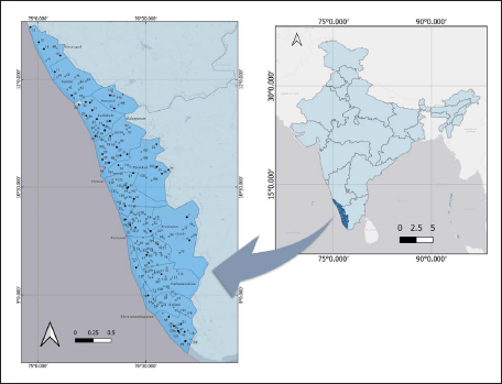
The state of Kerala is situated in the south-western part of the Indian sub-continent; it has a geographic extent of 38,863 km² constituting only about 1% of the total area of the country and is divided into 14 districts. The state is bordered by the apex of Western Ghats hill range on the eastern side and by the Arabian sea on the western side. It has a unique nature, with a high population density and a higher Human Development Index (HDI) in contrast to most of the other Indian states. With a GER of 38.7 (All-India GER is 26.3), Kerela is ranked 8 among 36 states and union territories in the country (MHRD, 2020). With an institutional density¹ of 45, which is much higher than the Indian national average of 28, the higher education scenario in Kerala is found to be placed in a better position than some of the rapidly expanding higher education systems in the southern states (Tilak, 2016). However, systematic studies are lacking in assessing the region-wise educational opportunities in India, particularly in the higher education sector, employing geospatial analyses.

In this context, it is necessary to understand the distribution of HEI across the state of Kerala and to identify localities where institutions are in oversupply, thereby providing better educational opportunities, and also those that are experiencing undersupply of HEIs.

The objective of the study is to identify and classify the geography of educational opportunity available in the study area. An important group of tertiary-level institutions is taken for this study, and for meeting the stated objective, the following three phases of study is conducted:

Using geospatial technique, identify and assess the present distribution of educational opportunity within the state of Kerala based on the degree of opportunity (choice of institutions available) for a group of institutions.

Integrate the opportunity areas identified in terms with similar studies or models made elsewhere.

Propose a re-creatable spatial-metric tool for classifying educational opportunity areas.

The aforementioned research questions are addressed by identifying the educational opportunity regions of (a) no choice or only one institution available and (b) abundance of choice of institutions, within the closely accessible distance of travel for a learner.

Data and Methods

According to the All-India Survey on Higher Education Report (2020), Kerala has 1,892 institutions in the higher education sector (universities, colleges and standalone institutions) with 1,417 colleges. The undergraduate colleges in the state form the largest group of institutions in the tertiary education sector. They are categorised mainly into government, aided and self-financing sectors. Based on the nature of the programmes offered, these institutions are classified into arts and science colleges, professional colleges and teacher education colleges.²

The data of the study include only those public-funded³ institutions, that is, arts and science in the government and aided sectors, which offer general⁴ undergraduate (bachelor’s degree) programmes. This category of college offers programmes in arts, humanities, sciences, social sciences and commerce disciplines. They are affiliated to the universities in the state, and follow a common procedure of admission and administration. Colleges of specialised nature such as Arabic, music and Sanskrit colleges have been excluded from the study. The sample therefore consists of 202 colleges, of which 148 belong to the aided sector and 58 to the government sector.

The study is predominantly concerned about the location of the institutions and the catchment area of each institution, which corresponds to its geographic reach. The first part of the study involves the demarcation of the geographic reach/coverage/catchment area of all institutions. The term ‘catchment area’ of an institution here denotes the optimal geographic distance from which an institution ‘admits’ or ‘catches up’ its students. For this purpose, we fix the buffer zone around each institution based on a fixed radius. Although the accessibility of an institution from a student’s place of residence is influenced by the type of terrain in which the institution is located, such aspect has not been considered in our study.

The entire geospatial analysis is carried out by using⁵ Arc GIS version 9.3.

The mapping and data processing are done as follows:

The raw data of 202 colleges⁶ obtained from the government-administrative sources contain only the physical address. They are converted to the corresponding geo-coordinate values⁷ (Table available)—latitude and longitude—by geocoding using ezGeocode of Google Workspace Marketplace. A map showing the location of institutions is generated and is shown in Figure 1.

The next step is to assign given value for drawing a buffer zone, applicable to every institution in the study. We have assigned a radius of 15 km as the standard value to draw circles around institution. This would be treated as the optimal catchment area of an institution. This has been arrived at based on a student’s access (average travel distance), for which the following rationale is employed after referring to the previous studies of similar aspect.

There is no conceptually well-defined radius that scholars use, hence a methodology was formulated based on previous studies of college proximity measured as ‘commuting distance, that is, the median distance a student was from their stated first-choice college. The median distance was shorter for urban students than for rural students (López Turley, 2009). Another example is the average city commute to work as 18.8 miles, and ‘nearby’ colleges within a 20-mile radius for the students in cities—double that distance for students outside of cities (González Canché, 2018); a city-centric multiple ring buffer of a 1–4=mile radius for finding college desert and oasis (Dache-Gerbino, 2018), although a standard buffer distance, the threshold (or ‘break-even distance’) may vary substantially from student to student (Frenette, 2006). A Eurostudent⁸ project on student’s commuting time and its implications observes that median time for travelling from home to the higher education institution (for one way only) for students who are living with their parents is 36 minutes across all countries (Schirmer et al., 2017, pp. 1–3).

In view of the earlier findings, this study has adopted a round-off duration of 30 minutes⁹ as the mean daily travelling time (one way) from a student’s home to the college. This 30-minute duration has been extrapolated to a corresponding distance of 15 km in fixing the buffer area of a college. The estimation of this distance is based on the prevailing average running time of 1 km in 2 minutes, which is applicable in the state for public transport buses as implemented by the Transport Authority (Kerala Government, 2018). The catchment area of an institution has been therefore determined as the distance algorithm, which is the 15-km mean radius, and has been used as the standard value to draw buffer circles around the institutions.

A map representing the catchment area of each of the 202 institutions, which is the buffer zone of 15 km radius, was generated (Figure 2).

Figure 1.

Source: The authors.

Figure 2.

Source: The authors.

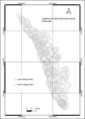
No specific pattern of distribution of institutions can be observed on the map and the buffer circles intersect each other at different places within the map, resulting in the formation of layers of varying sizes, degrees of overlap and frequency of occurrence across the area of study.

In order to understand the spread of geography of opportunities of these 202 institutions, the following explanation is provided and is explained with the help of Figure 3.

Figure 3.

Source: The authors.

In Figure 3 it is assumed that there are three institutions (C1, C2 and C3) located nearby, whose catchment areas are represented by circles (A₁, A₂ and A_3, respectively). First, circles are drawn around these institutions with a radius of 15 km. In this figure, the circles overlap in equal dimension. Since the layers are collections of geographic data, every segment of overlap can be treated as a layer, and the degree of overlap varies across the area of study. The segment formed from the overlap of three circles is denoted as Layer 3 and the segment formed due to the overlap of two circles is denoted as Layer 2. Those segments of circles remain without any overlap are denoted as Layer 1. Hence, each layer type in this case represents the corresponding choice of institution (alternatives) available within a distance of 15 km.

In the same figure, since Layer 1 and Layer 2 occur in three instances, they have a frequency of 3, whereas Layer 3, which occurs only once, has a frequency of 1. In the same way, these notations are extrapolated to the larger dimension of the study area where varying layer types and frequencies may occur.

Therefore, geospatial technique helps to find out (a) how many layer types (degree of opportunity/overlap/alternatives or choices of institutions) are possible; (b) frequency of each layer type (number of times in which the same layer type exist in the study area (which denotes the nature of geographic distribution of that layer); (c) cumulative area of each layer type (sum of the areas of layer frequency), which is the area of geographic distribution of a layer; and (d) percentage of area of each layer type against the total geographic extent of the study area.

We can compute the region of overlap of any finite number of circles under consideration, say, where n is a positive integer and is finite. This region lies within a 15-km radius of the n circles, and so it is the common region of overlap of the n circles.

Weightage values are assigned to the layer depending on the degree of overlap. For example, a weightage of 1 is assigned to the portion of circle that has no overlap area; weightage of 2 to area formed by overlap of two circles and so on.

Subsequently, the sum total of the area of weightage 1 (frequency of occurrence of Layer 1), weightage 2, weightage 3 and so has been determined as described further:

The present analysis has treated Layer 0 as a single unit.

Let Ni denotes frequency of Layer i,

For each i = 2, 3, ………., 15,

Let Aj (Li) denote the area of overlap region j of i circles, where j = 1, 2, ……, Ni and Li denotes Layer i.

Total area of Layer i (i.e., total area where there is access to i colleges)

\begin{array}{l} = A (L i) \\ = \sum_{i = 1}^{Ni} A j (Li), i = 2, 3, \dots, 15 \\ Total overlapping area = \sum_{i = 2}^{15} \sum_{i = 1}^{Ni} Aj (Li) \end{array}

In other words, the educational opportunity available to a student of a region is quantified in terms of layer types and their frequencies. The cumulative area (in sq.km scale) of the same layer type formed across the study area can be treated as the total spatial distribution of the corresponding educational opportunity.

Results

The geospatial analysis provided the following information of (a) number of layer types, (b) range of frequencies of layer types, (c) cumulative area of each layer and (d) percentage of area of a layer to the total geographic extent of the study area, which is shown in Table 1.

Table 1.

Description of Resulting Components and the Corresponding Values Obtained by the Geospatial Method Used.

(1)	(2)	(3)	(4)
Layer Type (Degree of Overlap/Alternatives)	Frequency of Occurrence	Area Occupied (Sq.km)	Percentage to the Total Area (%)
0	1	6,940.07	17.86
1	68	6,260.7	16.11
2	143	6,791.38	17.48
3	233	5,022.31	12.92
4	332	4,037.19	10.39
5	350	2,480.09	6.38
6	338	2,001.64	5.15
7	312	1,307.67	3.36
8	294	1,127.51	2.90
9	284	784.6	2.02
10	260	670.9	1.73
11	203	684.5	1.76
12	123	446.13	1.15
13	63	186.03	0.48
14	28	81.42	0.21
15	9	37.17	0.10
16	1	3.69	0.01

Source: The authors.

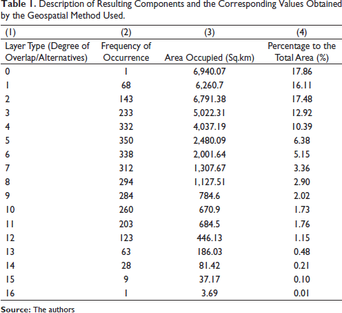
Table 1 shows the total number of layers formed, ranging from 0 to 16. It can be interpreted that Layer 1 has a frequency of 68, whereas Layer 16, the layer with the highest degree of opportunity, has a frequency 1. This means that the students who reside within Layer 16 have 16 institutions available within a travel distance of 15 km from the place of their residence. On the contrary, students residing within Layer 1 have only one institution available within a travel distance of 15 km from their place of residence. Therefore, Table 1 shows that there are regions of least alternatives and of several alternatives.

It is observed that after the demarcation of the layers, there is a blank area, which are regions that have no access to colleges within a travel distance of 15 km. These blank regions are taken as a single unit and is denoted as Layer 0.

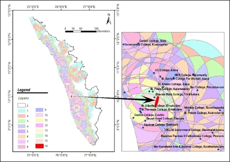
From the earlier results, it is evident that, although the degree of opportunity is very high for Layer 16, its geographic distribution is negligibly small as its frequency is 1. Due to the space constraints of this article, only the enlarged view of Layer 16 and its location is marked and shown (Figure 4).

Figure 4.

Source: The authors.

However, in order to reach a more meaningful explanation regarding the layers we have adopted the classification termed ‘Typology of Local Higher Education Markets’ (Hillman & Boland, 2019), which is shown in Figure 5. They defined a local higher education market by using the U.S. Department of Agriculture’s commuting zone classifications, in which it is mentioned that since students choose a college based on its proximity to home and work, these 709 commuting zones represent the “local” community from which students might search for a college.

Figure 5.

Source: Hillman and Boland (2019).

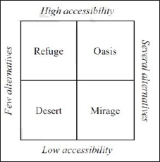
In the earlier typology, the two defining features of a local higher education market were described in which the horizontal axis represents the total number of colleges located in a commuting zone. The left side of this continuum represents commuting zones with the fewest alternatives nearby, where prospective students either have no or only one alternative from which to choose. On the right side of this continuum are commuting zones that offer multiple alternatives—places where students have a wider array of options from which to choose. Therefore, it is suggested that while some places may be ‘deserts’ with no available options, others may be ‘oases’ where opportunities are plentiful; other places with minimal opportunities may be ‘refuge’, and places where opportunities appear plentiful but are not are ‘mirages’.

Applying the metaphors of Typology of Local Higher Education Markets of Hillman and Boland to the present study, we now assign the terms to the layers as follows:

The area of Layer 0 and Layer 1 constitute the regions of no or least educational opportunities, respectively. This is in conformity with the previous definition of Education Desert, that it could either be (a) access deserts, the area where there is either zero college or that represent areas of the country that do not host the basic types of public institutions we would want students to have nearby; (b) match deserts, if they do not have access to a college that is academically matched to their academic credentials (Klasik et al., 2018; Robinson, 2018); or even (c) choice deserts (Blagg & Chingos, 2016; Hillman & Weichman, 2016), when there is only one public-broad-access college. Therefore, Layer 0 can be considered as access desert and Layer 1 as Choice Desert.

Therefore, the combined area of Layer 0 and Layer 1 constitutes the education desert. These are regions of no or least educational opportunity available.

However, since Layer 2 to Layer 16 indicate a wide range of degrees of opportunity and corresponding frequencies, it is necessary to classify them to suit to the other three classes in the Typology of Local Higher Education Markets.

We have therefore adopted cluster analysis¹⁰ using the centroid clustering method with the K-means clustering algorithm. Since the K-means clustering algorithm computes centroids and repeats until the optimal centroid is found, it is found to be the best method for our grouping. The three clusters formed by this method are shown in Figure 6.

Figure 6.

Source: The authors.

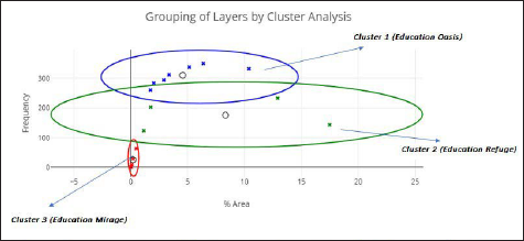
The three clusters are (a) Cluster 1: Layer 4 to Layer 10; (b) Cluster 2: Layer 2, 3 and 11, 12; and (c) Cluster 3: Layer 13 to 16.

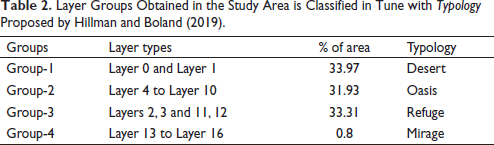
Therefore, these clusters can be placed into the typology framework of Hillman and Boland, which is shown in Table 2, and is explained further.

Table 2.

Layer Groups Obtained in the Study Area is Classified in Tune with Typology Proposed by Hillman and Boland (2019).

Groups	Layer Types	% of Area	Typology
Group-1	Layer 0 and Layer 1	33.97	Desert
Group-2	Layer 4 to Layer 10	31.93	Oasis
Group-3	Layers 2, 3 and 11, 12	33.31	Refuge
Group-4	Layer 13 to Layer 16	0.8	Mirage

Oasis: Group-2 consisting of Layer 4 to Layer 10, which forms the regions of high alternatives or choices coupled with large geographic area.

Refuge: Group-3 consisting of Layer 2, 3 and 11,12, in which, Layer 2 and Layer 3 have moderate to larger geographic distribution but with lesser alternatives or choice of institutions whereas, Layer 11 and 12 constitute moderate geographic distribution but with several alternatives or choices.

Mirage: Group-4 consisting of Layer 13 to 16. They appear as regions of numerous alternatives or choices, but are confined to a small area.

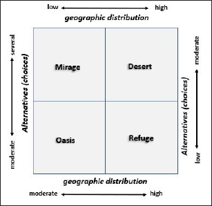
Based on the earlier results, we have recreated the typology in which the x-axis corresponds to the geographic distribution, which ranges from ‘low to high’, and y-axis represents the choice of alternatives, which ranges from ‘low to several’. Hence, the metaphors in the typology of Hillman and Boland have been adopted and modified to suit the geography of opportunity of the study area, shown in Figure 7.

Figure 7.

Source: The authors.

The corresponding spatial area occupied by each class of the typology, with respect to the total geographic extent of the study area (i,e., the state of Kerala) is shown in the pie-chart (Figure 8).

Figure 8.

Source: The authors.

Discussion

Kerala’s progress in achieving social well-being by all measures, ranging from the HDI to the Multi-Dimensional Poverty Index (MPI) and the Global Hunger Index (GHI) are not only decades ahead of India, but on par with the middle level  high-income countries (Chathukulam & Tharamangalam, 2021). In similar line, Kerala is better positioned in Sustainable Development Goals (SDGs), School Education Quality Index (SEQI) and other educational development index (Niti Ayog, 2021).

Despite the high level of literacy, near universal enrolment in elementary education, and high level of social and human development, J. B. G. Tilak (2001) opined that neglect of higher education is the principal reason for Kerala being positioned behind other states in India in economic development, whereas Simister (2011) opined that education is necessary, but not sufficient, for development. Unique geographic diversity also prevents the equity and access to higher education in the state. Tripathi (2019) identified that a combination of certain social as well as spatial and physical conditions continue to prevent equity of access to higher education and that the impeding factors like hilly terrain not only make transport facilities difficult, thereby affecting accessibility, but also obstruct satellite connectivity in institutions located in such regions. The establishment of institutions in the state over the years were influenced mostly by various socio-political considerations, rather than any specific demographic criteria or demand-based studies resulting in an uneven distribution of HEIs.

In this study, we propose a re-created tool for assessing the geographic distribution of education opportunity of a region.

From the re-created typology of higher education opportunities, some key observations are made. An optimal fixed distance that a student is expected to travel to their institution is the primary aspect of consideration and, accordingly, the study areas are demarcated into regions of negligible and abundant educational opportunities. Refuge constitutes 33.3%, which is a considerably higher geographic distribution of low to moderate choice of institutions. On the other hand, oases also cover a moderate geographic extent (31.93%), which offers a moderate to high choice of institutions also. As oases is spread over a large area of an administrative region, it can be considered as a satisfactory achievement in terms of equity and access. Equity and better access to some extent is therefore evident in the aforementioned two areas. Mirage are areas that indicate high institutional density but with smaller geographic distribution. Though this area has a high density of institutions and may seem to be an ideal ‘place’ of educational opportunity, it is not so as it as a smaller spatial extent and confined to only a single place. Even though students who belong to such regions have more options to choose their institution, a larger section of eligible population outside such the region cannot not receive such a benefit. It has also been observed that this mirage area is located in urban parts, supporting the fact that HEIs are mostly concentrated in urban areas (Varghese et al., 2018). This goes against the principles of equity.

Another important typology class delineated in this study is deserts. They are characterised by the absence or least opportunity of access to institutions. It has been observed that the deserts are confined to the eastern part of the study area, which can be attributed to the fact that this region mainly falls under forest cover (which forms 29% of the state) and comparatively inaccessible parts of Western Ghats. This means, the deserts, which constitutes nearly 34% of the study area, could also include some segments outside the boundaries of the forest cover. Only further studies can reveal the need of any expansion of educational opportunity to such regions.

As the state has nearly 1,600 HEIs of different types and categories (MHRD, 2020), a more detailed examination about such regional disparity in education opportunities is necessary.

The present study is an initial attempt to demarcate a geographic region into areas of educational opportunity, based solely on the institution’s catchment area. Similarly, if we couple our results with other factors such as population density, socio-economic elements, nature of terrain, lack of facility in public transport, digital divide, inaccessibility to healthcare system, and research and infrastructure, a larger dimension of assessment can be made.

There is an urgent need to evaluate whether the present scale of dispersion of institutions in the state is sufficient to address the educational need of students from all sections of society, particularly in the context of rising demand for a much higher GER.

Conclusion

The present study has used geospatial analysis to examine the scale of distribution of educational opportunities of the arts and science colleges in Kerala, which forms the major group of public institutions in tertiary education. The obtained results of regions of opportunity have been integrated with a previous model of geography of higher education choices, with minor modifications. We propose this modified spatial-metric tool using the Typology for Higher Education Opportunities for the State of Kerala, India. This tool can be re-created for similar studies with different of analytical variables. The method presented in our study identifies the areas of least and several opportunities of institutions. This kind of analysis will support the administrative and policy decision-makers in higher education by ensuring access and equity.

Footnotes

Declaration of Conflicting Interests

The authors declared no potential conflicts of interest with respect to the research, authorship and/or publication of this article.

Funding

The authors received no financial support for the research, authorship and/or publication of this article.

Notes

ORCID iD

Manulal P. Ram

Authors’ Bio-sketch

Manulal P. Ram, is currently working as an Research Officer in State Higher Education Council, Kerala India on deputation basis from the post of Assistant Professor in Geology Government College Kottayam. His core area of research focuses on Paleoclimatic studies but constantly works on Outcome Based Education and Policy Interventions in Higher Education sector.

Deepika Lakshman is an Assistant Librarian at Cochin University of Science and Technology (CUSAT) Ernakulam, Kerala, India presently working as Documentation Officer, Kerala State Higher Education Council, Thiruvananthapuram, Kerala India.

A.N. Manoharan, is an Assistant Professor in Department of Geology, Government College, Kasaragod, Kerala, India, is specialised in Geospatial Analysis and Water Resource Management.

Resmi Varghese is an Assistant Professor, Department of Mathematics, St. Xavier’s College for Women, Aluva, Kerala, India.

References

Alm

, & Winters

J. V.

(2009). Distance and intrastate college student migration. Economics of Education Review , 28(6), 728–738. https://doi.org/10.1016/j.econedurev.2009.06.008

Blagg

, & Chingos

M. M.

(2016). Choice deserts: How geography limits the potential impact of earnings data on higher education . Urban Institute. http://hdl.voced.edu.au/10707/431744

Cabrera

A. F.

, & La Nasa

S. M.

(2000). Understanding the college-choice process. New Directions for Institutional Research , 2000(107), 5–22. https://doi.org/10.1002/ir.10701

Chathukulam

, & Tharamangalam

(2021). The Kerala model in the time of COVID19: Rethinking state, society and democracy. World Development , 137, 105207. https://doi.org/10.1016/j.worlddev.2020.105207

Dache-Gerbino

(2018). College desert and oasis: A critical geographic analysis of local college access. Journal of Diversity in Higher Education , 11(2), 97–116. https://doi.org/10.1037/dhe0000050

Denzler

, & Wolter

(2011). Too far to go? Does distance determine study choices? (IZA Discussion Paper 5712). https://doi.org/10.2139/ssrn.1849467

(2004). The effects of local colleges on the quality of college attended. Economics of Education Review , 23(3), 249–257. https://doi.org/10.1016/j.econedurev.2003.05.001

Frenette

(2004). Access to college and university: Does distance to school matter? Canadian Public Policy , 30(4), 427–443.

Frenette

(2006). Too far to go on? Distance to school and university participation. Education Economics , 14(1), 31–58. https://doi.org/10.1080/09645290500481865

10.

Gibbons

, & Vignoles

(2012). Geography, choice and participation in higher education in England. Regional Science and Urban Economics , 42(1–2), 98–113. https://doi.org/10.1016/j.regsciurbeco.2011.07.004

11.

González Canché

M. S.

(2018). Nearby college enrollment and geographical skills mismatch: (Re)conceptualizing student out-migration in the American higher education system. Journal of Higher Education , 89(6), 892–934. https://doi.org/10.1080/00221546.2018.1442637

12.

Griffith

A. L.

, & Rothstein

D. S.

(2009). Can’t get there from here: The decision to apply to a selective college. Economics of Education Review , 28(5), 620–628. https://doi.org/10.1016/j.econedurev.2009.01.004

13.

Guzman

L. A.,

, Oviedo

, & Rivera

(2017). Assessing equity in transport accessibility to work and study: The Bogotá region. Journal of Transport Geography , 58, 236–246. https://doi.org/10.1016/j.jtrangeo.2016.12.016

14.

Hillman

, & Boland

W. C.

(2019). Geography of college choice. In contemporary issues in higher education (1st ed., p. 13). Routledge. https://doi.org/10.4324/9780429438127-2/GEOGRAPHY-COLLEGE-CHOICE-NICHOLAS-HILLMAN-WILLIAM-CASEY-BOLAND

15.

Hillman

, & Weichman

(2016). Education deserts. Viewpoints , 01–24. http://www.acenet.edu/news-room/Documents/Education-Deserts-The-Continued-Significance-of-Place-in-the-Twenty-First-Century.pdf%0Ahttp://www.acenet.edu/news-room/Pages/CPRS-Viewpoints-Education-Deserts.aspx?mkt_tok=3RkMMJWWfF9wsRonu6vNeu/hmjTEU5z17O4vUKa1

16.

Hillman

N. W.

(2014). Differential impacts of college ratings: The case of education deserts [Unpublished paper, University of Wisconsin-Madison].

17.

Hoyle

, & Knowles

(1998). Transport geography: An introduction. In Modern Transport Geography (2nd rev. ed.; pp. 1–12). John Wiley & Sons.

18.

Kerala Government. (2018). Decision of the meeting of the State Transport Authority . Transport Commissionerate, Government of Kerala.

19.

Klasik

D.,

, Blagg

, & Pekor

(2018). Out of the education desert: How limited local college options are associated with inequity in postsecondary opportunities. Social Sciences , 7(9), 165. https://doi.org/10.3390/SOCSCI7090165

20.

Lin

J. J.,

, Huang

Y. C.

, & Ho

C. L.

(2014). School accessibility and academic achievement in a rural area of Taiwan. Children’s Geographies , 12(2), 232–248. https://doi.org/10.1080/14733285.2013.812308

21.

Long

B. T.

(2004). How have college decisions changed over time? An application of the conditional logistic choice model. Journal of Econometrics , 121(1–2), 271–296. https://doi.org/10.1016/j.jeconom.2003.10.004

22.

López Turley

R. N.

(2009). College proximity: Mapping access to opportunity. Sociology of Education , 82(2), 126–146. https://doi.org/10.1177/003804070908200202

23.

Ministry of Human Resource and Development. (2020). AISHE final report 2019–20. In MHRD, India . MHRD.

24.

Niti Ayog. (2021). Annual report 2021–2022-Niti Ayog . NITI AAYOG.

25.

Niu

S. X.

, & Tienda

(2008). Choosing colleges: Identifying and modeling choice sets. Social Science Research , 37(2), 416–433. https://doi.org/10.1016/j.ssresearch.2007.06.015

26.

Nyoni. (2017). Factors affecting students’ academic achievement in Zimbabwe’s rural secondary schools: A case study of Marimasimbe Secondary School in Jiri community. Dynamic Research Journals’ Journal of Economics and Finance , 2(March), 1–15.

27.

Ogechi

I.,

, Snook

K.,

, Davis

B. M.,

, Hansen

A. R.,

, Liu

, & Zhang

(2016). Pet ownership and the risk of dying from cardiovascular disease among adults without major chronic medical conditions. High Blood Pressure and Cardiovascular Prevention , 23(3), 245–253. https://doi.org/10.1007/s40292-016-0156-1

28.

Robinson

J. A.

(2018). The curious case of so-called ‘higher education deserts.’ James G Martin Center for Academic Renewal.

29.

Rouse

C. E.

(1995). Democratization or diversion? The effect of community colleges on educational attainment. Journal of Business & Economic Statistics , 13(2), 217. https://doi.org/10.2307/1392376

30.

Schirmer

H.,

, Orr

, & Gwosc

(2017, February). Intelligence brief: Students’ commuting time its implications . Eurostudent project: Supporting the social dimension of higher education.

31.

Simister

(2011). Assessing the ‘Kerala model’: Education is necessary but not sufficient. Journal of South Asian Development , 6(1), 1–24. https://doi.org/10.1177/097317411100600101

32.

Skinner

B. T.

(2019). Choosing college in the 2000s: An updated analysis using the conditional logistic choice model. Research in Higher Education , 60(2), 153–183. https://doi.org/10.1007/s11162-018-9507-1

33.

Sørensen

E. S.

, & Kamp

(2016). Does distance determine who is in higher education? (Munich Personal RePEc Archive Working Paper 74517). https://mpra.ub.uni-muenchen.de/74517/

34.

Sponsler

B. A.

, & Hillman

(2016, April). Where you live rather than what you know ? The problem with education deserts . Brookings. https://www.brookings.edu/blog/brown-center-chalkboard/2016/04/11/where-you-live-rather-than-what-you-know-the-problem-with-education-deserts/

35.

Tilak

J. B. G.

(2001). Higher education and development in Kerala. In Center for Socio-Economic and Environmental Studies: Vol. February (Issue 5). http://csesindia.org/admin/modules/cms/docs/publication/5.pdf

36.

Tilak

J. B. G.

(2016). How is Kerala doing in higher education? Rajagiri Journal of Social Development , 8(1), 3–18. https://doi.org/10.13140/RG.2.1.1570.7368

37.

Tripathi

(2019). Higher education in Kerala: Development, equity and issues of access. South Asia Research , 39(3/Suppl), 42S–60S. https://doi.org/10.1177/0262728019872054

38.

Turley

R. N. L.

(2006). When parents want children to stay home for college. Research in Higher Education , 47(7), 823–846. https://doi.org/10.1007/s11162-006-9017-4

39.

Varghese

N. V.,

, Panigrahi

, & Rohatgi

(2018). Concentration of higher education institutions in India. Centre for Policy Research in Higher Education , 110016(October), 1–74.

40.

White

P. M.

, & Lee

D. M.

(2020). Geographic inequalities and access to higher education: Is the proximity to higher education institution associated with the probability of attendance in England? Research in Higher Education , 61(7), 825–848. https://doi.org/10.1007/s11162-019-09563-x