Simulating individual work trips for transit-facilitated accessibility study

Abstract

To measure job accessibility, person-based approaches have the advantage to capture all accessibility components: land use, transportation system, individual’s mobility and travel preference, as well as individual’s space and time constraints. This makes person-based approaches more favorable than traditional aggregated approaches in recent years. However, person-based accessibility measures require detailed individual trip data which are very difficult and expensive to acquire, especially at large scales. In addition, traveling by public transportation is a highly time sensitive activity, which can hardly be handled by traditional accessibility measures. This paper presents an agent-based model for simulating individual work trips in hoping to provide an alternative or supplementary solution to person-based accessibility study. In the model, population is simulated as three levels of agents: census tracts, households, and individual workers. And job opportunities (businesses) are simulated as employer agents. Census tract agents have the ability to generate household and worker agents based on their demographic profiles and a road network. Worker agents are the most active agents that can search jobs and find the best paths for commuting. Employer agents can estimate the number of transit-dependent employees, hire workers, and update vacancies. A case study is conducted in the Milwaukee metropolitan area in Wisconsin. Several person-based accessibility measures are computed based on simulated trips, which disclose low accessibility inner city neighborhoods well covered by a transit network.

Keywords

Geographic information systems accessibility agent-based modeling work trip transit simulation

Background

The ultimate goal of transportation is to enable people to access opportunities including employment, resources, services, recreation, etc. (Litman, 2012). Accessibility has been continuously studied by scholars and planners. Although a majority of accessibility studies has focused on automobile transportation, transit-facilitated accessibility has gained popularity in recent years (Djurhuus et al, 2016; Lei and Church, 2010; Mavoa et al., 2012; Salonen and Toivonen, 2013).

Accessibility is defined as people’s ease to reach potential opportunities using a particular transportation system (Dalvi and Martin, 1976; Hansen, 1959). It has been studied from a spectrum of perspectives including transportation infrastructure (Gutierrez and Urbano, 1996), land use (Geurs and Ritsema van Eck, 2003; Hansen, 1959), mobility of people (Handy and Niemeier, 1997; Kwan, 1998; Miller, 1991, 1999), locations (Leonardi, 1978), access to jobs (Hanson and Schwab, 1987; Sanchez et al., 2004; Shen, 1998), and resources (Mavoa et al., 2012). A host of accessibility measures have been developed based on different perspectives and focuses, among which person-based accessibility measures have gained interests because they are capable of capturing all four accessibility components which include land use, transportation, individual person, and time (Geurs and van Wee, 2004).

However, person-based accessibility measures face a number of challenges. First, they require detailed individual travel data which are extremely difficult and costly to obtain (Geurs and van Wee, 2004; Kwan, 1998, 1999; Miller, 1991, 1999). Standard travel surveys normally do not provide the necessary individual’s time budget (Miller, 1999; Thill and Horowitz, 1997). Second, person-based approaches often do not account for competition effects (Geurs and van Wee, 2004) given that they are usually based on limited number of respondents. Also due to limited data availability, applications are often constrained to relatively small areas and specific social groups. Third, a framework that links individual behavior to long-term land use changes does not exist (Waddell, 2001) given that models are often based on short-term activities. So far, this situation has not been substantially changed.

Person-based approaches are more appropriate for transit-facilitated accessibility measures than traditional approaches because traveling using transit involves person-related constraints, e.g. availability of cars and time constraints, and personal choice. In addition to the lack of individual trip data, modeling transit trips has more challenges than modeling automobile trips because schedule-based path-finding capability is not currently supported by standard geographic information systems (GIS) and there is even no standard GIS data format for transit. To date, research in transit-facilitated accessibility has been rare.

This paper presents a model that simulates work trips of individuals who depend on transit in an attempt to explore the potential of using simulated trip data for accessibility study. The rest of the paper is organized as the following: “Literature review” section reviews literature of accessibility study and agent-based modeling (ABM); “Methodology” section presents an agent-based model and describes the agents involved; “The case study area and data” section describes a case study area; “Results” section discusses accessibility measures derived from simulated individual trip data of the case study area; and finally “Conclusion and discussion” section concludes findings and discusses a few issues.

Literature review

A host of accessibility measures designed for various problem domains can be found in the literature. Kwan (1998) notes that person-based space–time approaches are able to capture activity-based contextual effects which are not reflected in traditional location-based accessibility measures, and they allow more sensitive assessment of individual variations in accessibility. Geurs and van Wee (2004) evaluate accessibility measures and conclude that person-based measures have great theoretical advantages since “they satisfy almost all theoretical criteria”.

The pioneering work of individual activity-based accessibility study can be attributed to Lenntorp’s (1978) space–time accessibility measures based on Hägerstrand’s (1970) time–geographic framework. Using hypothetical individual activities, Lenntorp measures the volume of space–time prism, i.e. Potential Path Space (PPS) which is defined by the two-dimensional space for activity locations and one dimension of time. Based on the PPS, a Potential Path Area (PPA) which is the projection of the three-dimensional PPS on the two-dimensional space is measured. Lenntorp’s model assumes a uniform space and constant travel speed.

While the majority of the literature on accessibility studies focuses on automobile transportation, transit-oriented accessibility study is much underrepresented although it has gained interest in recent years. Huang and Wei (2002) study public transport provided accessibility based on a traditional aggregate model. Liu and Zhu (2004a, 2004b) develop a GIS software package that facilitates various accessibility measures based on static transportation networks including bus routes and stops. In both studies, the transit levels of service measures are static indicators while individual trips and schedule coordination are not considered. Lei and Church (2010) define an extended GIS data structure to handle temporal elements of transit service and develop travel time-based accessibility measures. Given an arrival or departure time, isochrones from an origin or destination location are computed as spatial measure of accessibility. Although schedule coordination is fully incorporated in computing the isochrones, personal and opportunity factors are ignored. In addition, isochrones is essentially PPAs. Using PPA to measure transit-facilitated accessibility is arguable because an actual accessible area is limited within a tolerable walking distance (commonly 400 meters) of bus stops (Langford et al., 2012). Similar to Lei and Church (2010), Djurhuus et al. (2016) elaborate a multimodal network model that supports time-table-based trip planning. The network is used to determine individual accessibility by public transportation. Given an individual’s home address and a time budget (30, 45, or 60 minutes), it computes an accessibility area that accommodates all trip components and restrictions. In both Djurhuus et al. (2016) and Lei and Church (2010), land use is ignored and only one individual factor, time budget, is considered. Other individual factors such as mobility, competition and preference are not included.

To integrate all four accessibility components, simulating individual trips using ABM should provide a promising alternative to mass data acquisition. ABM is a technology that models individual elements of a system as agents (Batty, 2003). When all agents of a system are deployed, the pattern of the system emerges as a result of interactions of the underlying components (Jackson et al., 2008). An agent is a self-contained individual that have goals, can make decisions, and is able to exhibit goal-directed behavior (Teweldemedhin et al., 2004). An agent can perceive its environment and behave by following rules. Moreover, by fine tuning parameters, an agent may be endowed with personality (Doniec et al., 2008). In transportation simulation, for example, a driver agent may be characterized as normal, cautious, or aggressive (Khalesian and Delavar, 2008). Furthermore, agents may have social ability (Teweldemedhin et al., 2004) such as to communicate with other agents, to learn, and to compete with one another.

Based on the notion to make use of readily available national data without additional data collection especially specific trip diary, Veldhuisen et al. (2000, 2005) describe a microsimulation model RAMBLAS that simulates daily activity patterns in the context of a regional planning to predict traffic flows on a transportation network for various times of the day using relatively simple principles. The model is implemented in the Eindhoven region in the Netherlands, in which the synthetic population is based on Monte Carlo simulation and activity agendas are drawn at random from the national distribution. Shortest paths between residential zones of agents and their destinations are used in simulating trips. Three planning scenarios including regional scenario, national scenario, and do-nothing scenario are simulated to reveal number of dwellings to build, population characteristics, and traffic characteristics.

Lovelace et al. (2014) describe a microsimulation of individual commuting. The model assigns simulated micro-data (individuals) to geographic zones of census by repeatedly adjusting a large array of weights to maximize the fit between simulated and census data. Then the simulated individuals are related to the nearest employment center to create origin-destination pairs. Once individuals and job locations are simulated, resulted micro-level commuting data can be aggregated at any geographic scale to display travel patterns such as aggregated distance to employment centers, employment density of job centers, popular commuter destinations, as well as route choice of the simulated individuals, etc.

Babakan and Alimohammadi (2016) and Babakan and Taleai (2015) describe an agent-based model to investigate the impacts of transportation development on residence choice of renter households in Tehran, Iran. In the study, renter households are treated as agents that can make multi-objective decisions and compete with one another in renting preferred residential zones. A None-dominated Sorting Genetic Algorithm II (NSGA-II) is employed for agents to evaluate residential options by maximizing utility and minimize disutility. A synthetic population of 50,000 renter households is generated using Monte Carlo simulation in 560 traffic analysis zones in Tehran and three transport development scenarios are simulated. Computation is conducted in MATLAB. While no specific transportation mode is focused in these simulations, Ciari et al. (2013) introduce an activity-based microsimulation of carsharing for Zurich, Switzerland. A synthetic population of agents are created and deployed in a virtual world. Each agent has a number of socio-demographic attributes and its daily activity plan describing the chain of activities. Activity chains are assigned to each agent according to its socio-demographic attributes. Several plans are evaluated for each agent and the highest score is retained and used to create new plans based on the agent’s previous experience. The simulation is implemented by MATSim, an open source agent-based simulation software. Result shows that carsharing accounts for 0.6% of transportation demands in the simulation.

Transit is an important transportation mode especially for unprivileged groups in inner cities although it has been underrepresented in transportation research literature. While most existing research aim at travel demand, mode split or traffic flows, simulating individual activities using transit is even rarer. Liu and Zhou (2016) describe an agent-based integer linear formulation to represent capacity constrained transit service network in which agents are used to travel in capacity constrained transit networks in order to understand their path choice and travel time. However, no personal objective or social behavior is simulated for agents.

Methodology

Agent-based modeling

This research uses ABM technology to simulate the commuting patterns of transit-dependent workers. Like other microsimulation models, a synthetic population is first generated based on census data. The model simulates the population as three levels of agents: census tracts, households, and individual workers, each will be explained soon in this section. Unlike some studies that use general employment centers or zones for destinations (Babakan and Taleai, 2015; Veldhuisen et al., 2000, 2005), job opportunities are simulated as agents as well with precise locations. These agents have properties and behaviors. Once they are deployed, they start to play and we can observe the trip activities of each individual worker agent.

As an experimental system, the following rules and assumptions are made to minimize the complexity. First, this simulation focuses on transit-dependent workers. Workers commuting by other transportation modes are not simulated. Second, job opportunities within walking distance to bus stops are included in the system while those beyond the distance are excluded. Like Djurhuus et al. (2016), a 1-kilometer walking distance is adopted in the case study although 400 meters is commonly used in transportation analysis. Third, peak hour delays are accommodated in the time table of the transit system and all buses are assumed to run on schedule. Forth, buses have no capacity limit so that all simulated agents can get on any desired vehicle. This assumption can generally stand in cities with low-transit ridership. Finally, except for competing for jobs, no other social behaviors such as learning and communication will be modeled for worker agents. The following explains agents simulated in this study.

Census tract agents

Census data are the basis for population simulation and census tract is the geographic unit in which population agents are generated. A census tract agent has a polygon shape and a number of demographic properties including total population, number of households, total labor force, civilian labor force, civilian employed labor force, civilian unemployed labor force, total number of workers, workers by trip mode (six categories), workers by industry of employment (13 categories), etc. A census tract agent has the ability to generate household agents and worker agents based on its demographic profile. First, it randomly generates household agents along roads based on residential density which is specified by a weight field in the road feature class. Then, based on the number of workers commuting by transit, it generates transit-dependent worker agents and randomly assigns them to households within 1 kilometer distance to bus stops. Priority is given to households with no cars or low in income in the assignment.

Household agents

A household agent maintains properties including location, census tract identifier, number of cars, income level, and a collection of persons. Household agents are used to hold persons and link simulated worker agents to census tracts. No social behavior is simulated for the household agent in this research.

Worker agents

A worker agent has basic properties of a person such as sex and age category, and it has job related properties including industry of employment, work trip mode, employer identifier, etc. It is an active agent that can search for jobs, competing with other agents for jobs, and can find the best commuting path by transit.

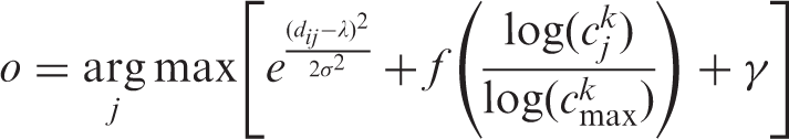
A worker agent searches for jobs based on four factors: industry of employment, perceived distances to job locations, attractiveness of job opportunities, as well as a luck (stochastic) factor. It evaluates each job opportunity (employer agent) in the industry it works in and scores the opportunity based on the four factors. The one that ranks the highest is finally assigned to the worker agent. In this process, the perceived distance is represented by the Euclidean distance between the worker agent’s home and an opportunity location. This should be fine since a perceived distance does not have to be perfectly accurate but it is computationally much more efficient than the network distance. In scoring, the distance factor is evaluated by a Gaussian function in which the mean is determined by the most suitable commuting distance by transit. Statistics New Zealand (2006)¹ notes a mode of 2 to 5 kilometers in travel distance by transit. The attractiveness of opportunities is indicated by the ratio of employment capacity of an employer to the capacity of the largest employer of the industry in the region. Job search scoring is expressed by the following function

o = \arg_{j} max [e^{\frac{(d_{ij} - λ) 2}{2 σ^{2}}} + f (\frac{\log (c_{j}^{k})}{\log (c_{max}^{k})}) + γ]

where o is the job opportunity (employer) selected by worker agent i, d_ij is the Euclidean distance between the agent’s home and opportunity j, λ is the most suitable transit distance, σ is the standard deviation of transit distance,

c_{j}^{k}

is the capacity of employer j of industry k,

c_{max}^{k}

is the capacity of the largest employer of industry k in the region. f is a scaling function which is not used in this research. Variable γ is a random number representing the luck factor. The value range of each component is calibrated between 0 and 1, and priorities can be controlled by fine-tuning parameters.

To enable path finding by worker agents, a transit trip planning module supported by a schedule-based path finding algorithm (Huang, 2007; Huang and Peng, 2008) is integrated in the simulation system. For each work trip, the total travel time includes walking time from the origin (home or workplace) to the starting transit stop, riding time, transfer time, and walking time from the end transit stop to the destination (workplace or home). While O-D matrix may be pre-calculated for walking time (Djurhuus et al., 2016), walking time is calculated on the fly in this simulation. Given the gridiron street pattern in the case study area, Manhattan distance is used to estimate walking times. For a distance of 30 meters or less, a 1-minute walking time is used; for a distance between 30 and 100 meters, a 2-minute walking time is used. For a distance of 100 meters and more, the walking time is estimated as 2 minutes plus the time to cover the distance beyond 100 meters at a speed of 4.5 kilometers/hour.

Employer agents

An employer agent has a location, a business name, and a NAICS code (industry category). It maintains a total number of employees, a capacity for transit-dependent workers, as well as the number of transit-dependent workers hired. With a limited capacity for hiring transit-dependent workers, competition between worker agents in job search is enabled. Once a worker agent is hired by the employer, one vacancy is deducted from the capacity at the employer.

The capacity for transit-dependent workers at each employer is estimated based on the percent of transit trips among all trips in the region and a lottery mechanism. In the case study area of this research, for example, transit-dependent workers accounts for 4.19% of all workers (ACS 2007–2011) which is about one out of 24 employees. However, many small businesses have less than 24 employees thus may not be assigned a transit-dependent worker at all if only the proportion is used in the assignment. To properly estimate capacity for transit-dependent workers at all businesses, a lottery mechanism based on Gaussian distribution is employed

e_{t} = x + α \cdot (E - x) \cdot γ

x = max {n \in ℤ | n \leq E \cdot r_{t}}

where e_t is the capacity for transit-dependent employees of an employer, E is the total number of employees of the employer, r_t is the ratio of transit trips to all trips of the region, x is the integer part of E · r_t, α is a constant coefficient, and γ is a Gaussian random number.

Transportation

Two transportation data sets are required for the simulation: street centerlines and transit data. The former is used for generating household locations. A household density field is created to control agent density. By default, roads in single-family neighborhoods are assigned a density of 1.0. High residential density roads are assigned with values greater than 1.0. Value 0 is assigned to unpopulated roads such as expressways and roads in industrial zones or in public open spaces. Transit dataset is a SQL database that stores bus routes, stops, trips, schedules, etc. It also defines a transit network by maintaining relationships between transit elements. A transit trip planner uses the network to find the best work trip paths for worker agents. A transit network data model is described in Huang and Peng (2008).

Model structure and implementation

A class diagram for the simulation system is shown in Figure 1. This model consists of five classes that are used to define agents, a transit trip planner module, and an output database. The CensusTract class has a number of properties defining a demographic profile. It has two methods: GenerateHouseholds generates household agents and GenerateWorkers produces worker agents. The Household class maintains basic information of a household. It has a method for adding persons into the household.

Figure 1.

Structure of the agent-based simulation model.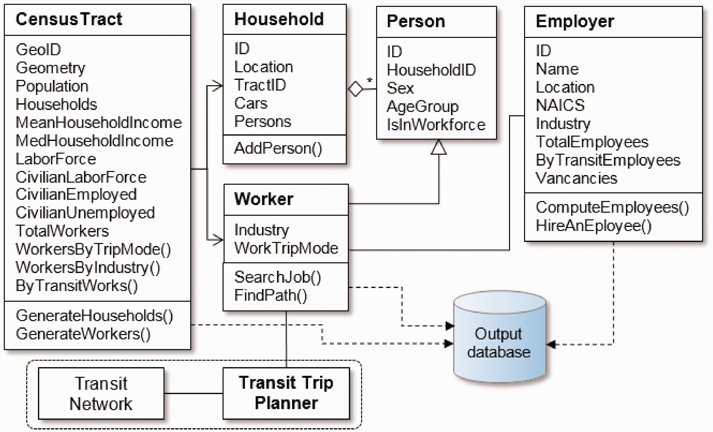

A person class is used to maintain individual person data. It has properties including sex, age category, workforce status, household identifier, etc. No social behavior is currently simulated. The Worker class inherits the Person class, and maintains work-related properties including the industry of employment and work trip mode. It has a SearchJob method and a FindPath method. A transit trip planner module is associated with the Worker class to enable worker agents to find best paths in a transit network. It also has the ability to find the shortest path in a road network. The employer class maintains a location, industry, NAICS, total number of employees, number of transit-dependent employees, as well as number of vacancies. The ComputeEmployees method estimates the number of employees using each transportation mode for work trips, and the HireAnEmployee method handles hiring and updates the number of vacancies.

The simulation system uses a SQL database to store outputs including all agents generated, the employment status and employer of each worker agent, worker agents hired by each employer, as well as detailed trip data of the worker agents. Simulated trip data includes agent ID, planned departure time or expected arrive time, total travel time, walking time, ride time, transfer time, number of transfers, a path shape, transfer locations, as well as trip directions.

An ArcGIS Desktop extension called Agent-Based Transit Accessibility Simulator (ABTRASM) is developed using.NET programming and the Esri ArcObjects library. This extension includes an ArcMap toolbar and a dockable window. Computation for the case study (“The case study area and data” and “Results” sections) was completed on a desktop PC with a Pentium quadcore CPU of 3.0 GHz clock frequency and 8 GB of RAM. With a relatively large system including 81 bus routes, 7071 bus stops, and 27,044 transit-dependent worker agents, computation time is about 9 hours for one run (one trip for each agent). The computer is able to process four parallel sessions.

Accessibility measures

Travel time is a key measure of accessibility provided by transit (Lei and Church, 2010; Liu and Zhu, 2004b) as well as an essential part of the analysis of accessibility disparity between different travel modes (Salonen and Toivonen, 2013). In this study, a simulated trip consists of all time components of a typical transit trip including to/from bus stops, riding time, and transfer time. Moreover, an agent can be set to commute at different times so that the minimum, maximum, and average commuting times of the agent are available. Accessibility measures can be developed by aggregating individual data by any geographic unit or demographic categories. “Mean minimum travel time by industry” through “Driving time and transit time” sections discuss a few accessibility measures based on a case study.

Validation

Simulation of individual activities is by nature so detailed that validation is challenging because detailed information needed for the validation is virtually never available for an entire region (Lovelace et al., 2014). One way to validate the model is to aggregate simulation results to a level at which aggregated survey data are available. Particularly, simulated individual commuting times are aggregated by census tracts and then validated against the American Community Survey (ACS) estimates. “Result validation” section further discusses validation simulation results.

The case study area and data

A case study is conducted for the Milwaukee metropolitan area in Wisconsin. In 2010, the area has a population of 1.34 million in 512,859 households. Based on the ACS 2011 five-year estimate, the total number of workers in the area is 634,342. Transit service is provided by two transit systems: the Milwaukee County Transit System (MCTS) and Waukesha Metro Transit (WMT). The joint transit network consists of 81 bus routes and 7071 bus stops (Figure 2), and it operates 4949 bus trips on a weekday.

Figure 2.

The Milwaukee-Waukesha metropolitan area.

Bus ridership in this area is low with 4.19% of workers commute by public transportation (ACS 2007–2011). However, bus ridership varies significantly among neighborhoods. Figure 2 shows that inner cities have higher percentage of transit-dependent workers than other areas including downtown. The percent of transit-dependent workers in some north inner city census tracts are 16% and higher. Milwaukee is a hypersegregated city in which high minority concentration inner cities have badly suffered from poverty and inequality (Smith, 2013). Due to continuous budget cut thus bus service reduction since 2000, more and more suburban job opportunities have become inaccessible by transit which has raised serious concerns (Rast, 2011).

Population simulation and agent generation in this study are based on data of the US Census 2010 and ACS 2007–2011 (5-year estimate). Employer agents are generated based on 2011 US business data which maintains business name, address, NAICS, revenue, employees, etc. All business establishments in the study area are first address located. A total of 36,751 establishments within 1 kilometer from any bus stop are selected to create employer agents. Based on NAICS, employers are classified into 13 categories following the ACS industry classification (Table 1).

Table 1.

Industry classification and coding used in this study.

Code	Industry
AGR	Agriculture, forestry, fishing and hunting, and mining
REC	Arts, entertainment, recreation, accommodation, food service
CON	Construction
EDU	Education, health care, social assistance
FIN	Finance, insurance, real estate, rental, and leasing
INF	Information
MAN	Manufacturing
PRO	Professional, scientific, management, administrative, waste management
PUB	Public administration
RET	Retail trade
TRA	Transportation, warehousing, utility
WHO	Wholesale and trade
SER	Other services (except public administration)

Results

In the case study, a total of 27,044 transit-dependent worker agents are generated. Each agent is set to travel from home to workplace (work-trip) with 13 departure times between 6:00 and 9:00 at 15 minute intervals, and from workplace to home (home-trip) with 13 departures between 16:00 and 19:00 at 15-minute intervals. A total of more than 540,000 trips are generated with an overall mean of 44.19 minutes for work trips and 45.04 minutes for home trips. These mean travel times agree with the national averages which are about 48 minutes for departures between 7:00 and 7:59 a.m. and 45 minutes after 4:00 p.m. (ACS: Commuting in the United States 2009).²

Commuting time by transit is determined by the spatial layout of employment opportunities, home locations, and the transit system, which are reflected in travel distance and transit level of service. Travel time-based accessibility measures can be derived from individual’s minimum or mean travel time aggregated by industry or census tracts.

Mean minimum travel time by industry

Assuming every worker agent is able to choose a departure time that minimizes total travel time, the mean minimum travel time of worker agents in a specific industry is derived from

{\bar{t}}_{1} = \frac{\sum_{j} [min (t_{ij})]}{n_{i}}

where t is work trip time, i indicates industry, j represents individual worker agents, min(t_ij) is the minimum work trip time for agent j of industry i, and n_i is the number of transit-dependent worker agents in industry i. Results are shown in Table 2.

Table 2.

Mean minimum travel time (minutes) of individual worker agents by industry.

Industry	Work trip			Home trip
Industry	Mean	SD	Valid trips	Mean	SD	Valid trips
AGR	26.82	17.95	22	27.18	17.93	22
REC	37.90	18.45	900	38.79	18.84	886
CON	39.18	18.87	3502	38.43	19.82	3465
EDU	32.00	13.57	536	31.85	13.89	518
FIN	35.83	16.63	2685	35.86	16.46	2625
INF	40.27	20.21	1035	35.94	21.09	747
MAN	41.37	24.14	489	39.36	23.57	464
PRO	32.52	14.53	1617	31.62	13.52	1581
PUB	32.66	14.62	2364	31.99	14.93	2300
RET	32.38	15.64	5711	32.15	15.60	5591
TRA	33.30	17.70	2497	33.28	17.68	2419
WHO	31.76	13.69	1109	31.47	13.64	1058
SER	30.01	10.48	766	29.88	10.21	747

Theoretically, long work trip times can occur to industries with clustered job opportunities and shorter work trip times occur in industries with scattered job opportunities. In Table 2, the top three industries requiring long work-trip times include manufacturing (41.37 minutes), information (40.27 minutes), and construction (39.18 minutes), and the top three industries with long home-trip times are manufacturing (39.36 minutes, recreation (38.79 minutes), and construction (38.43 minutes). Figure 3 shows job opportunities in the construction industry clustered in the downtown area and alongside major transportation corridors (Figure 3).

Figure 3.

Clustered job opportunities in the construction industry accessible by transit.

Although the industry of agriculture, forestry, fishing, etc. (AGR) displays short travel times, this industry may not be statistically significant as it has a very small number (157) of transit-dependent worker agents which produce only 22 valid trips. Excluding AGR, industries with relatively short travel times include services (except public administration), wholesale, education, retail, and public administration (Table 2). A significant characteristic of these industries is that job opportunities are scattered throughout the region.

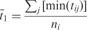
Mean minimum and average travel times by census tracts

Since not every worker has the freedom to travel at the most convenient time, the average travel time of a worker agent during the simulation period is also a good indication of accessibility. To reveal spatial patterns of transit-facilitated accessibility, the means of individual agent’s minimum and average travel times for each census tract are calculated (Figure 4). It is not surprising that peripheral areas show longer travel times than the central city in all measures since the central city concentrates employment opportunities of many industries. However, the inner cities clearly display longer travel times than their surrounding areas in all measures. Inside the 6-kilometer radius circle in the maps, inner city neighborhoods consistently display higher commuting time clusters.

Figure 4.

Mean work trip time (circle radius 6 km). (a) Mean minimum work-trip time, Moran’s I = 0.0717; p value = 0.0000; (b) Mean average work-trip time; Moran’s I = 0.0796; p value = 0.0000; (c) Mean minimum home-trip time, Moran’s I = 0.1004, p value = 0.0000; (d) Mean average home-trip time, Moran’s I = 0.0782, p value = 0.0000.

Number of transfers and high-transfer rate

Transferring between routes can significantly increase the total time of a trip. In transportation modeling, transfers can affect model choice. Therefore, number of transfers can be used as a measure of accessibility as well. In this study, the average number of transfers in all valid trips is 0.68. Assuming all agents choose to travel by the minimum-transfer path, the minimum-transfer trips of worker agents are retrieved from the result database. In the case study, 44.73% of the agents need no transfer, and 43.42% of agents require one transfer. The number of agents requiring different number of transfers are listed in Table 3.

Table 3.

Agent minimum-transfer commuting trips.

Transfers	Work-trip		Home trip
Transfers	Agents	Percent	Agents	Percent
0	9949	44.73	10,001	45.20
1	9657	43.42	9600	43.39
2	1833	8.24	1788	8.08
3	755	3.39	730	3.30
4	41	0.18	7	0.03
5	5	0.02	0	0.00
Total	22,240	100.00	22,126	100.00

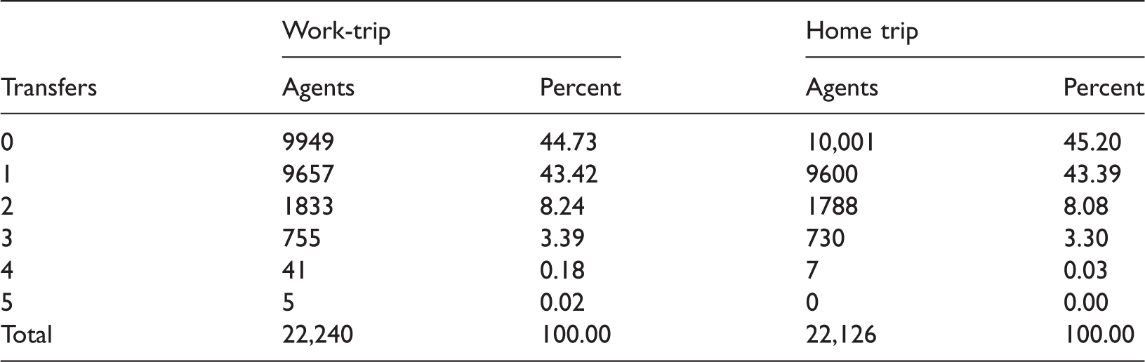
To disclose the spatial distribution of high-transfer agents, a high-transfer rate (HTR), i.e. the percent of trips requiring two or more transfers among all valid trips, is computed by census tracts and mapped in Figure 5. For both work trip (Figure 5(a)) and home trip (Figure 5(b)), clusters of high HTR values appear in the inner cities, which indicates inner city residents need more transfers to access job opportunities by transit.

Figure 5.

High-transfer rate (circle radius 6 km). (a) Work trip; (b) Home trip.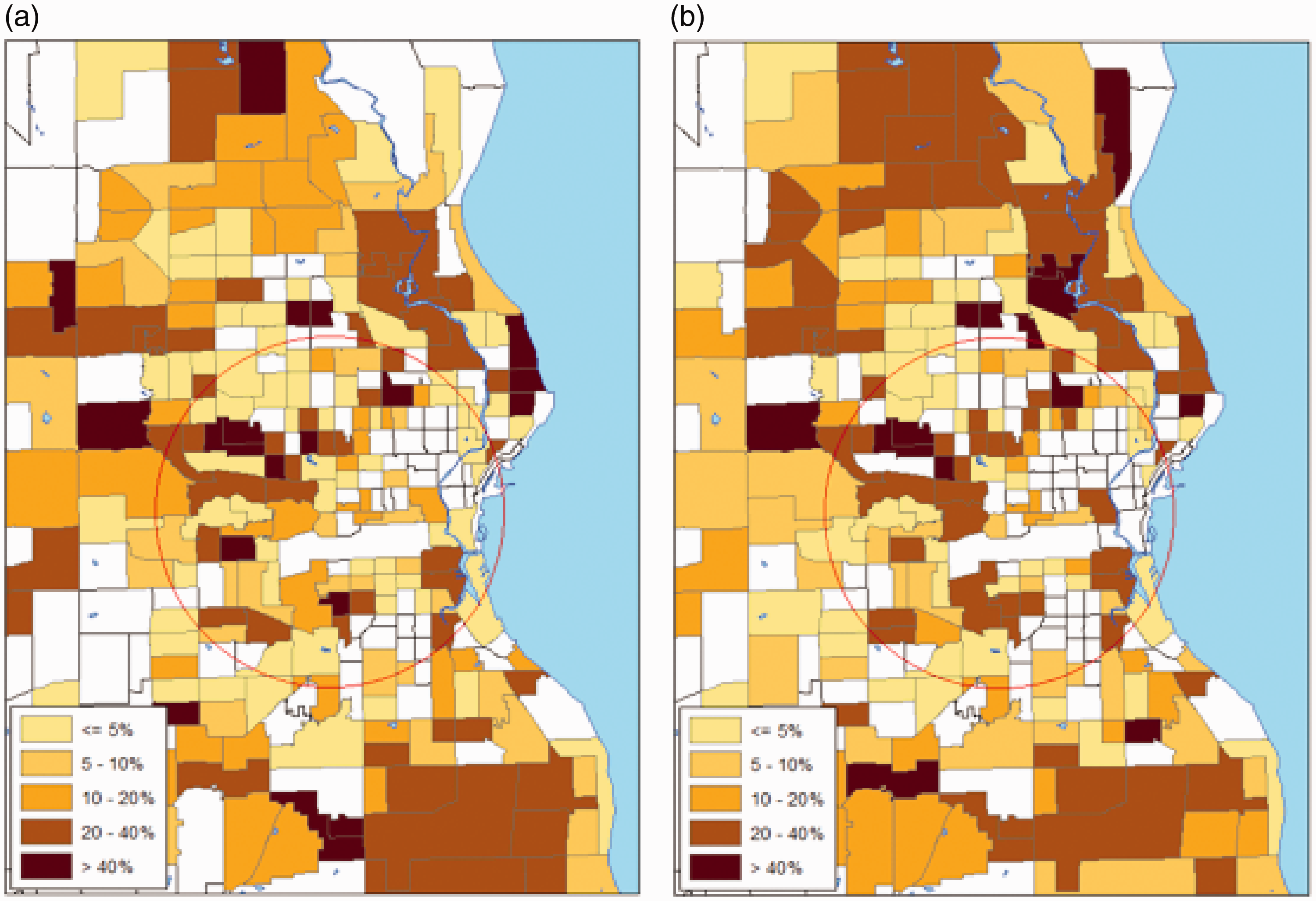

Driving time and transit time

Assuming driving is an option to every worker; this study also computes the driving time for worker agents so that a comparison between transit time and driving time is possible. Driving time is derived from road speed limits and distance of the fastest path of each agent. Congestion is not simulated because of the lack of data. Although driving time derived this way may not be realistic, especially for peak hours, it is a general indication of commuting distance. Figure 6(a) shows the mean driving time of work trips by census tracts. Again, the map displays a significant clustering of relatively high driving time in the inner cities, suggesting that inner city agents have to travel longer distance to reach job opportunities.

Figure 6.

Work-trip mean transit time and driving time. (a) Driving time, Moran’s I = 0.1334, p value = 0.0000; (b) Min transit/driving time, Moran’s I = 0.1240, p value = 0.0000.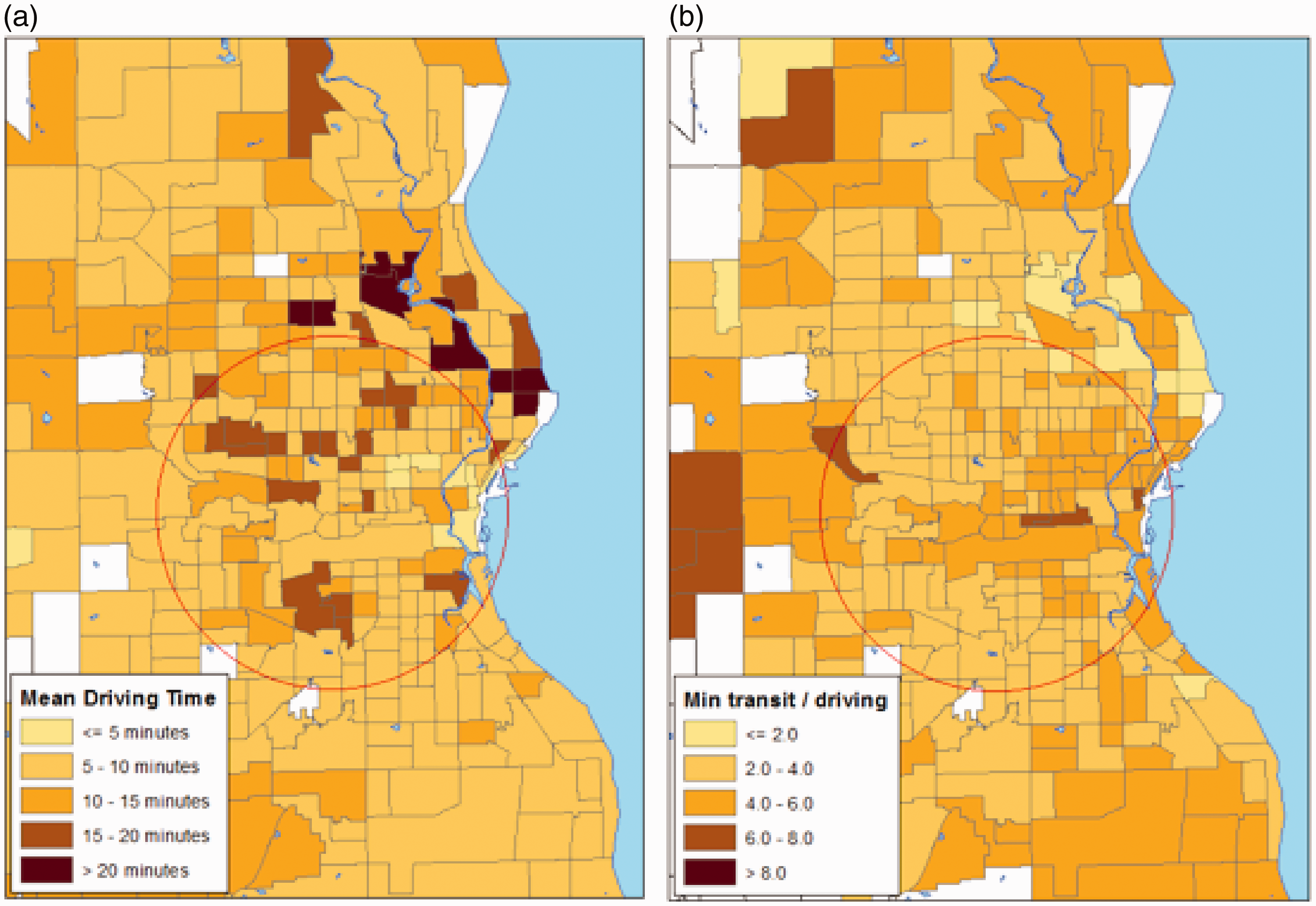

Generally, traveling by transit takes more time than by driving. In this study, the ratio of individual’s minimum transit time to driving time varies greatly with an overall mean of 4.04. The mean ratios by census tracts are presented in Figure 6(b). Interestingly, inner city neighborhoods show relatively lower ratios (2 to 4). This does not mean that public transportation is more convenient for these neighborhoods because traveling by transit still takes much longer time than driving. The relatively lower ratios may be due to the relatively longer commuting distances for inner city residents and the express lines that serve far destinations in the suburbs.

Result validation

Since detailed commuting survey data is not available for the study area, the simulation results are validated against the aggregated ACS 2007–2001 five-year estimates. First, the number of simulated transit-dependent worker agents by census tracts are plotted against the ACS surveys. In Figure 7, the horizontal axis represents the number of simulated transit-dependent workers in each census tract, and the vertical axis represents the ACS data of corresponding census tracts. A relatively good relationship is indicated by a moderate correlation coefficient (0.6621).

Figure 7.

Simulation vs. ACS: number of commuters by transit by census tracts (r = 0.6621).

Second, the overall mean work-trip time and home-trip time of all simulated agents agree well with the ACS surveys (see the first paragraph of “Results” section).

Third, categorized travel times are validated against the ACS. For each census tract, the ACS provides number of transit commuters in four travel time categories: less than 30 minutes, 30 to 44 minutes, 45 to 59 minutes, and 60 minutes and more. In this study, the simulated agents are categorized in the same way based on the minimum travel time of each agent and the results are plotted against the ACS data. In Figure 8, the less than 30 minutes category and 30–44 minutes category show fairly good relationships.

Figure 8.

Simulation vs. ACS: number of commuters by commuting time by census tracts.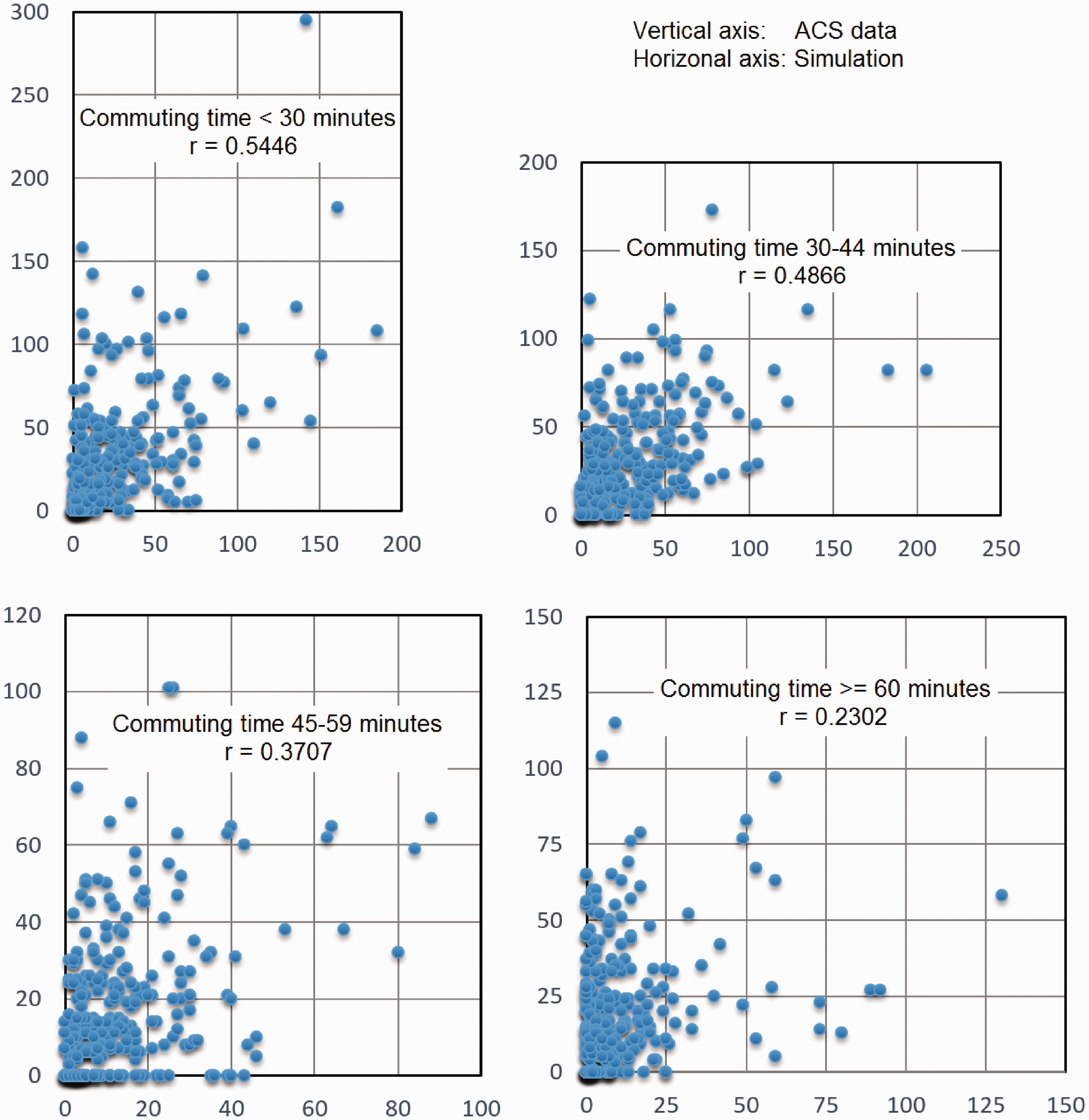

Conclusion and discussion

The paper presents an agent-based model for exploring transit-facilitated job accessibility using publicly existing data. The model simulates census tracts, households, individual workers, employers as agents. When the agents are deployed in a simulation, individual trip data including individual worker information, employer information, time of all trip components (accessing the origin transit stop, riding in the vehicle, transferring between routes, and walking from the end stop to destination), number of transfers, and path shapes. The driving distance and time of each worker agent are also produced. The detailed simulation data allow for development of accessibility measures aggregated by any geographic units or demographic categories.

A case study is conducted in the Milwaukee metropolitan area in Wisconsin. A total of 27,044 transit-dependent worker agents are generated, which produce more than 540,000 trips. First, the means minimum travel times of individual agents by industries are calculated. The result shows that agents in industries with clustered job opportunities have longer travel times than those in industries with scattered opportunities. Second, the mean minimum and average travel times of individual worker agents by census tracts are computed. These measures reveal a cluster of long commuting time neighborhoods inner cities. Third, HTR (the ratio of trips requiring two or more transfers among all trips) by census tracts are calculated. This measure also indicates a cluster of unprivileged neighborhoods in the inner cities. Finally, an assumed driving times for agents by census tracts are derived. These measures consistently suggest that inner city workers are unprivileged in job accessibility by transit although the neighborhoods are well covered by transit networks.

As a simple model, it demonstrates the feasibility of using publicly available data to simulate individual trips for accessibility studies. Since the focus of this study is work trips by transit, the model does not simulate sophisticated traveler behaviors such as chain trips and learning ability. These can be topics of future research if the model is to be expanded to include other transportation modes or activities. Because of the lack of detailed survey data for the case study area, validation has to use the aggregated ACS data. If surveyed individual trip data are available, model parameters can be refined and results can be better validated.

Footnotes

Declaration of conflicting interests

The author(s) declared no potential conflicts of interest with respect to the research, authorship, and/or publication of this article.

Funding

The author(s) received no financial support for the research, authorship, and/or publication of this article.

Notes

Ruihong Huang, PhD is an associate professor in geography at the Department of Geography, Planning, and Recreation of Northern Arizona University. His research interests include GIS data modeling and programming, GIS for transportation, and spatial modeling.

References

Babakan

Alimohammadi

(2016) An agent-based simulation of residential location choice of tenants in Tehran, Iran. Transactions in GIS 20(1): 101–125.

Babakan

Taleai

(2015) Impacts of transport development on residence choice of renter households: An agent-based evaluation. Habitat International 49: 275–285.

Batty

(2003) Agent-based pedestrian models. In: Longley

Batty

(eds) Advanced Spatial Analysis: The CASA Book of GIS, Redlands, CA: ESRI Press, pp. 81–106.

Ciari F, Schuessler N, Axhausen KW, et al. (2013) Estimation of carsharing demand using an activity-based microsimulation approach. Model discussion and some results: International Journal of Sustainable Transportation 7: 70–84.

Dalvi

Martin

(1976) The measurement of accessibility: Some preliminary results. Transportation 5: 17–42.

Djurhuus

Hansen

Aadahl

et al. (2016) Building a multimodal network and determining individual accessibility by public transportation. Environment and Planning B: Planning and Design 43: 210–227.

Doniec

Mandiau

Piechowiak

et al. (2008) A behavioral multi-agent model for road traffic simulation. Engineering Application of Artificial Intelligence 21: 1443–1454.

Geurs

Ritsema van Eck

(2003) Accessibility evaluation of land-use scenarios: The impact of job competition land-use and infrastructure developments for the Netherlands. Environment and Planning B 30(1): 69–87.

Geurs

van Wee

(2004) Accessibility evaluation of land-use and transport strategies: Review and research directions. Journal of Transport Geography 13: 127–140.

10.

Gutierrez

Urbano

(1996) Accessibility in the European Union: The impact of the Trans-European road network. Journal of Transport Geography 4(1): 15–25.

11.

Hägerstrand

(1970) What about people in regional science? People of the Regional Science Association 24: 7–21.

12.

Handy

Niemeier

(1997) Measuring accessibility: An exploration of issues and alternatives. Environment and Planning A 29: 1175–1194.

13.

Hansen

(1959) How accessibility shapes land use. Journal of American Institute of Planners 25: 73–76.

14.

Hanson

Schwab

(1987) Accessibility and intraurban travel. Environment and Planning A 19(6): 735–748.

15.

Huang

(2007) A schedule-based pathfinding algorithm for transit networks using pattern first search. GeoInformatica 11: 269–285.

16.

Huang

Peng

(2008) A spatiotemporal data model for dynamic transit networks. International Journal of Geographic Information Science 22(5): 527–545.

17.

Huang

Wei

(2002) Analyzing neighborhood accessibility via transit in a GIS environment. Geographic Information Science 8(1): 39–47.

18.

Jackson

Forest

Sengupta

(2008) Agent-based simulation of urban residential dynamics and land rent change in a gentrifying area of Boston. Transactions in GIS 12(4): 475–491.

19.

Khalesian M and Delavar MR (2008) A multi-agent based traffic network micro-simulation using spatio-temporal GIS. In: Proceedings of commission II, ISPRS Congress, Beijing, 3–11 July 2008.

20.

Kwan

(1998) Space-time and integral measures of individual accessibility: A comparative analysis using a point-based framework. Geographical Analysis 30(3): 191–216.

21.

Kwan

(1999) Gender and individual access to urban opportunities: A study using space–time measures. The Professional Geographer 51(2): 210–227.

22.

Langford

Fry

Higgs

(2012) Measuring transit system accessibility using a modified two-step floating catchment technique. International Journal of Geographical Information Science 26(2): 193–214.

23.

Lei

Church

(2010) Mapping transit-based access: Integrating GIS, routes and schedules. International Journal of Geographical Information Science 24(2): 283–304.

24.

Lenntorp

(1978) A time-geographic simulation model of individual activity programes. In: Carlstein

Parkes

Thrift

(eds) Human Activity and Time Geography Vol. 2, London: Edward Arnold, pp. 371–382.

25.

Leonardi

(1978) Optimum facility location by accessibility maximising. Environment and Planning A 10: 1287–1305.

26.

Litman T (2012) Evaluating accessibility for transportation planning. Available at: http://www.vtpi.org/access.pdf (accessed 25 July 2013).

27.

Liu

Zhou

(2016) Capacitated transit service network design with boundedly rational agents. Transportation Research Part B 93: 225–250.

28.

Liu

Zhu

(2004a) Accessibility analyst: An integrated GIS tool for accessibility analysis in urban transportation planning. Environment and Planning B: Planning and Design 31: 105–124.

29.

Liu

Zhu

(2004b) An integrated GIS approach to accessibility analysis. Transactions in GIS 8(1): 45–62.

30.

Lovelace

Ballas

Watson

(2014) A spatial microsimulation approach for the analysis of commuter patterns: from individual to regional levels. Journal of Transport Geography 34: 282–296.

31.

Mavoa

Witten

McCreanor

et al. (2012) GIS based destination accessibility via public transit and walking in Auckland, New Zealand. Journal of Transport Geography 20: 15–22.

32.

Miller

(1991) Modelling accessibility using space-time prism concepts within geographical information systems. International Journal of Geographical Information Systems 5(3): 287–301.

33.

Miller

(1999) Measuring space–time accessibility benefits within transportation networks: basic theory and computational procedures. Geographical Analysis 31: 1–26.

34.

Rast J (2011) An analysis of the impact of proposed 2012 Milwaukee County transit service reductions on access to employment. Available at: https://www4.uwm.edu/ced/publications/transitjobs_2011update.pdf (accessed 7 January 2017).

35.

Salonen

Toivonen

(2013) Modelling travel time in urban networks: Comparable measures for private car and public transport. Journal of Transport Geography 31: 143–153.

36.

Sanchez

Shen

Peng

(2004) Transit mobility, jobs access and low-income labour participation in US metropolitan areas. Urban Studies 41(7): 1313–1331.

37.

Shen

(1998) Location characteristics of inner-city neighbourhoods and employment accessibility of low-wage workers. Environment and Planning B 25(3): 345–365.

38.

Smith W (2013) Milwaukee – A Third World City. Daily Kos, 29 June. Available at: http://www.dailykos.com/story/2013/06/30/1220042/-Milwaukee-A-Third-World-City# (accessed 30 May 2015).

39.

Teweldemedhin E, Marwala T and Mueller C (2004) Agent-based modelling: A case study in HIV epidemic. In: Proceedings of the fourth international conference on hybrid intelligent systems (HIS’04). 0-7695-2291-2, Kitakyushu, Japan, 5–8 December 2004. IEEE.

40.

Thill

Horowitz

(1997) Travel time constraints in destination choice sets. Geographical Analysis 29: 108–123.

41.

Veldhuisen

Timmermans

Kapoen

(2000) RAMBLAS: A regional planning model based on the microsimulation of daily activity travel patterns. Environment and Planning A 32: 427–443.

42.

Veldhuisen

Timmermans

Kapoen

(2005) Simulating the effects of urban development on activity – Travel patterns: an application of Ramblas to the Randstad North Wing. Environment and Planning B: Planning and Design 32: 567–580.

43.

Waddell

(2001) Towards a behavioural integration of land use and transportation modelling. In: Hensher

(ed.) Travel Behaviour Research: The Leading Edge, Amsterdam: Pergamon, pp. 65–95.