Implementation and calibration of a new irregular cellular automata-based model for local urban growth simulation: The MUGICA model

Abstract

Cellular automata-based models have traditionally employed regular grids to represent the geographical environment when simulating urban growth or land use change. Over the last two decades, the scientific community has introduced the use of other spatial structures in an attempt to represent the processes simulated by these models more realistically. Cadastre parcels are a good choice when simulating urban growth at local scales, where pixels or regular cells do not represent the geographic space properly. Furthermore, the implementation and calibration of key factors such as accessibility and suitability have not been sufficiently explored in models employing irregular structures.

This paper presents a fully calibrated model to simulate urban growth: Model for Urban Growth simulation using Irregular Cellular Automata. The model uses the irregular structure of the cadastre and its smallest unit: the cadastral parcel. The factors included are based on the traditional Neighbourhood, Accessibility, Suitability and Zoning Status modelling schema, frequently employed in other models. Each factor was implemented and calibrated for the irregular structure employed by the model, and a new approach was explored to introduce a random component that would reproduce illegal growth. Several versions of Model for Urban Growth simulation using Irregular Cellular Automata were produced to calibrate the model within the period 2000–2010. The results obtained from the simulations were compared against observed growth for 2010, adapting the traditional confusion matrix to irregular space. A new metric is proposed, called growth simulation accuracy, which measures how well the model locates urban growth.

Keywords

Irregular cellular automata model calibration urban simulation urban growth

Introduction

Urban growth has become one of the main concerns in the world today. Some 54% of the world’s population currently live in urban areas, and this figure is predicted to rise to 66% in 2050 (United Nations, 2014). In recent decades, several authors have highlighted the need to prepare for urban growth in terms of planning policies (Bengston et al., 2004; Sakieh et al., 2015). In order to achieve this, more research is required to understand how cities work, determine the driving factors of growth (Herold et al., 2003), elucidate the consequences of different types of urban growth (Aguilera et al., 2010) and identify better alternatives to achieve sustainable futures (Herold et al., 2005).

One of the approaches that has successfully shed light on urban growth processes is the use of exploration tools such as simulation models. Of these, cellular automata (CA) models have demonstrated their capacity to effectively reproduce city characteristics such as emergence, self-similarity, self-organisation, and non-linear behaviour (Barredo et al., 2003). From the early applications to geographic phenomena (Tobler, 1970), through models with more developed factors (White and Engelen, 1993), to more complex models (Stevens and Dragicevic, 2007), the success of this kind of model in urban environments has been undeniable. CA models still maintain their essence, the Game of Life proposed by John Conway (Gardner, 1970), but currently present various modifications that have been added to the original structure over time in order to reproduce urban growth processes more precisely (Couclelis, 1997). These changes have brought with them the new term of CA-based models. From the possible set of modifications that a model can incorporate, the change in how space is represented and the smallest unit (cell) that a model could employ are still under discussion (Barreira-González et al., 2015a; Pinto and Antunes, 2010).

In this regard, CA-based models can be divided into two groups, according to how they represent space: (1) regular or raster CA-based models and (2) irregular CA-based models. The first group encompasses all models that employ regular grids to represent space, in which the cells, as well as pixels in satellite imagery, all present the same resolution and topology. These models, which are derived from the Cellular Geography proposed by Tobler (1979), have demonstrated their capacity to effectively describe and study urban processes at global scales (Santé et al., 2010). Nevertheless, the pixel/cell unit is not the best way to reproduce reality at local scales (Moreno et al., 2009). Changes at these scales are located at management units, such as plots, parcels, or other structures related to administrative purposes. Hence, although pixels in remote sensing images are linked to units of observation, they are not necessarily the appropriate unit for analysis of urban growth (Zelaya et al., 2016). In addition, CA-based models have not been incorporated into planning processes, partly due to the lack of communication between modellers and planners (Triantakonstantis and Mountrakis, 2012). The use of the same unit as that employed in urban development plans would improve the dialogue between modellers and planners, enabling the incorporation of these models into planning processes (Martín-Varés, 2009).

Although a few models have now successfully incorporated the irregular structure of the territory (Dahal and Chow, 2014; Moreno et al., 2008; Pinto and Antunes, 2010; Stevens et al., 2007), this remains a subject of research (Barreira-González et al., 2015a) and poses several challenges. The question of how to model typical CA-based model factors of urban growth, such as neighbourhood, suitability, accessibility, and zoning status (based on the Neighbourhood, Accessibility, Suitability and Zoning Status [NASZ] modelling schema proposed by White et al., 1997) in an irregular environment remains unexplored (Barreira-González et al., 2015a). The definition and effect of neighbourhood have been recently documented by several authors (Barreira-González and Barros, 2017; Dahal and Chow, 2015). Nevertheless, suitability, accessibility, zoning status and the random factor (often added to models to reproduce the uncertainty that social processes entail) have not been explored in irregular CA-based models.

The objective of the present study was to produce a fully functional irregular CA-based model capable of reproducing past urban growth and using the spatial unit employed in urban planning: the cadastral parcel. The model, named the Model for Urban Growth simulation using irregular (MUGICA), uses the NASZ schema with all factors fully developed for the irregular structure employed by the model. As part of model implementation, it was necessary to evaluate and calibrate each factor, testing their sensitivity. Thus, several versions of the model were produced using different factor implementation combinations. A total of 224 versions were run over the calibration period (2000–2010) and compared against observed urban growth for 2010. The version that presented the best fit was selected and the random factor was added to reproduce the uncertainty that social processes entail. Again, multiple versions of this version of the model (10) were obtained with different values for randomness, and these were run 100 times each for 2010.

The MUGICA: Materials and methodology

Study area and data sets

The Region of Madrid has been one of the most dynamic areas in Spain, and more generally in Europe, in terms of urban growth over the last two decades (Hewitt and Escobar, 2011; Plata Rocha et al., 2009). The Metropolitan Area of Madrid has grown beyond the limits of its own boundaries, merging with other cities or towns without any vacant space in between. This may indicate the need for urban plans involving several municipalities in a common planning process. In order to test the model presented here, three municipalities were selected (Meco, Los Santos de la Humosa and Azuqueca de Henares) in the east of the current functional Region of Madrid, which exceeds the official Region of Madrid and extends into the province of Guadalajara (Figure 1).

Figure 1.

Study area.

The study area is interesting due to the wide variety of differences between the three municipalities. Los Santos de la Humosa is located on a hill and still retains a very important rural component, while the other two are almost flat and have a motorway boundary that limits their growth. Their population, urban areas and socio-economic conditions are also dissimilar. What renders them even more interesting is that they form part of an important industrial corridor along the A-2 motorway (the Henares Corridor), reinforcing still further the need for common urban development planning policies.

The structure employed by MUGICA is the cadastre data set (General Directorate for Cadastre, 2013). In Spain, the cadastre represents the spatial structure of land ownership. The smallest unit is the cadastre parcel, and it thus seemed appropriate that this element should be the smallest unit employed by a model aimed at simulating urban growth. Land use for the years 2000 and 2010 was mapped by combining the cadastral data set and the historical satellite imagery available for most parts of the province of Madrid (NOMECALLES, 2016).

The core of MUGICA: Parameter and factor definition in irregular spaces

MUGICA has been fully developed in Python (Van Rossum, 2007), combining open source libraries for geospatial data such as Geospatial Data Abstraction Library (GDAL) (Fundation, 2008), with commercial libraries such as ArcPy from ArcGIS. Although several irregular CA-based models have been proposed to date, few studies have conducted an in-depth exploration of factor definition for irregular spaces (Barreira-González et al., 2015a; Barreira-González and Barros 2017; Dahal and Chow, 2015). As mentioned previously, MUGICA follows the NASZ schema proposed by White et al. (1997). This modelling schema includes several key factors that determine changes and growth: neighbourhood, suitability, accessibility and zoning status. Furthermore, many models add another random component so as to reproduce the uncertainty that these processes may entail: the random factor (García et al., 2011).

The model simulates urban growth for two land uses: residential and productive. The amount of area developed in each model iteration (one calendar year), commonly known as demand, is previously defined by the user for each land use. In the present study, demand was defined as the amount of residential and productive area developed over the period 2000–2010.

Neighbourhood

Neighbourhood is defined by proximity between spatial elements (parcels in irregular space), which depends on their spatial location and functional relationship (effects that one land use exerts on the others; Couclelis, 1997; Dahal and Chow, 2015; O’Sullivan, 2001). This intrinsic CA factor can be divided into two elements: definition and effect (Barreira-González and Barros, 2017).

CA-based models that use regular grids to represent geographical space usually employ the same size or shape of neighbourhood to identify those cells that would constitute the neighbourhood of a given cell. In the case of irregular CAs, neighbourhood definition is especially critical: the intrinsic irregularity of parcel size and shape renders the neighbourhood different for each parcel. The definition of neighbourhood in irregular CAs has been sufficiently well documented (Dahal and Chow 2015; Moreno et al., 2009; Stevens and Dragicevic, 2007). Most irregular CAs implement buffers around parcels and identify which parcels fall within these. Nevertheless, calibration of the distance at which the buffer should be generated is still the subject of debate due to the sensitivity of the model to this parameter. As can be seen, this is similar to the problem of neighbourhood size in regular CA-based models, indicating that results obtained from the model may be sensitive to changes in neighbourhood size (Kocabas and Dragicevic, 2006). In line with the methodology proposed by Barreira-González and Barros (2017), the neighbourhood of a parcel is defined in MUGICA as the region covered by the buffer generated around it, including parcels either fully or partially covered by the buffer. The model employs graph theory to represent parcels and neighbourhood.

Meanwhile, neighbourhood effect represents the effect, also known as the push-and-pull effect (Lau and Kam, 2005), that the land use in a cell exerts on the others according to the distance between them. In terms of mathematical representation, this effect is usually expressed as a distance–decay function for each pair of land uses. The greater the distance, the less the effect exerted. In regular CA-based models, these functions can be obtained using spatial metrics such as the Neighbourhood Index (Hansen, 2012) or Enrichment Factor (Verburg et al., 2004) and applying them at several distances. In the case of irregular spaces, these metrics can be adapted to this environment, as demonstrated by Barreira-González and Barros (2017), then derived and implemented within the models.

In MUGICA, the neighbourhood effect is modelled through distance-decay functions obtained from a previous study of the neighbourhood at different distances, quantifying the amount of area of the buffer that is covered by each land use. As the model simulates two classes of urban land use, there would be four kinds of function per set of functions: functions that represent the effect that residential use exerts on other locations to develop a residential (R to R) or productive (R to P) land use, and functions that represent the effect that productive use exerts on other locations to develop a residential (P to R) or productive (P to P) land use. The effect exerted by rural land is not included in these functions, since the amount of rural land is greater in comparison to urban land. It was tested, but the results showed that the function which was not affected by neighbourhood distance. Nevertheless, the effect of rural land is reproduced in the suitability map, where this type of land is taken into account.

Spatial metrics such as the Vector Enrichment Factor (vEF) and Vector Neighbourhood Index (vNI) were employed to obtain a total of four sets of distance–decay functions (A, B, C and D). Figure 2 shows the four sets of neighbourhood effect functions obtained for the study area. The set of functions A was obtained using the vNI, considering those parcels where urban land was developed between 2000 and 2010. Set B encompassed vNI values, considering all urban parcels in 2000. Set C was obtained using the vEF in its logarithmic form, considering those parcels where urban land was developed between 2000 and 2010. Set D encompassed vEF values in its logarithmic form, considering all urban parcels in 2000. The model is capable of using one of these sets of functions in each simulation. Sets A and C are used to study if there was a difference compared with the rest of parcels by employing only those that experienced change.

Figure 2.

Sets of neighbourhood effect functions.

Accessibility

Accessibility influences the organisation and dynamics of a region, and consequently the location of people and activities (Bavoux et al., 2005). This concept may have its origins in the earliest land use transport models (Wegener, 2004). It can be defined as the ease with which people can access given amenities or locations via the transport network (Gutiérrez, 2009). Thus, the combination of two elements defines the accessibility of a region: the location of destinations and transport network characteristics (Vickerman, 1974).

In order to measure ease of accessibility, Handy and Niemeier (1997) classified accessibility metrics into three categories: gravity-based metrics (accessibility decreases when travel time or distance increases), utility-based metrics and isochrones. Gravity-based metrics are the most suitable of these three groups for CA-based models, due to their ease of implementation in the models. Most CA-based models have often employed an approach similar to that proposed by White et al. (1997), whereby the accessibility value for a given cell is inversely proportional to the distance to the road network. In the case of irregular CAs, accessibility metrics can be easily computed through the road network as the travel time or distance to access given locations. Consequently, the model results may be affected by the target locations selected to calculate accessibility. Nevertheless, there is currently no optimum way to calculate or measure this factor (Vandenbulcke et al., 2009).

In the present study, four accessibility metrics were compared in order to select the one that best reproduced observed urban growth in the MUGICA calibration period: 2000–2010 (Figure 3). The first two metrics (1 and 2) were based on the travel distance from a parcel (in metres) along the road network to reach target locations: (1) was measured from the nearest node on the road network and (2) was measured from the nearest section of the road network. The second two metrics (3 and 4) were based on the travel time (in seconds) to access target locations using the road network: (3) was measured from the nearest node and (4) from the nearest section. Time can be computed from the speed limit on each road. Target locations were selected using principal nodes within the road network and main connections to motorways.

Figure 3.

Accessibility maps: each legend shows the accessibility metric that is being represented (1,2,3,4). Hot spots are the target locations to compute the metrics.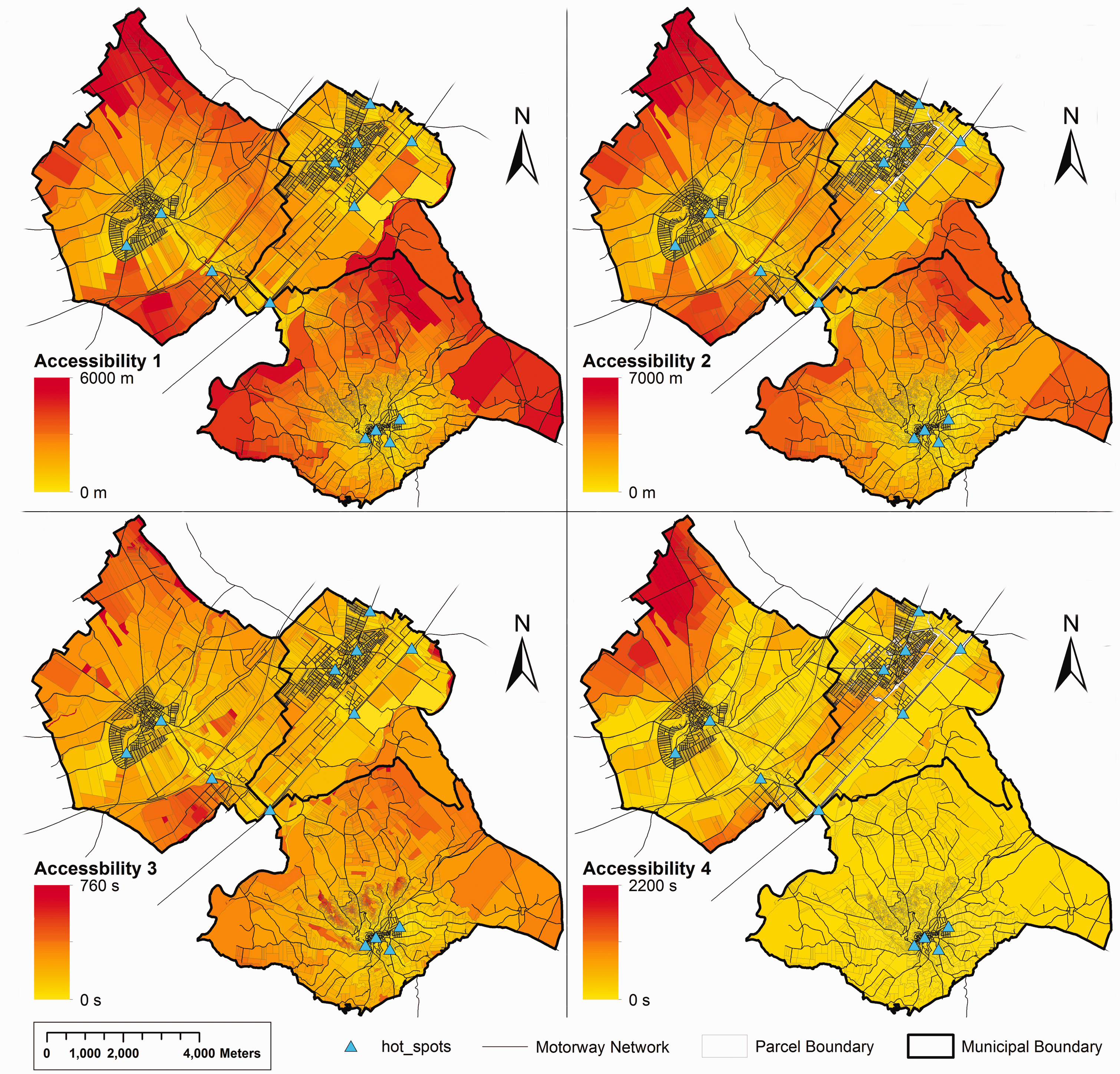

Suitability

The suitability of a cell to develop a land use is usually related to location factors and site properties (Li and Yeh, 2000). Mathematically, it can be understood as a deterministic linear function of several factors, which contribute to the evaluation of each location in the territory (Barredo et al., 2004). There is no consensus in the scientific community regarding the variables to include in this parameter (Barredo et al., 2003; Dahal and Chow, 2014; García et al., 2012), since they are dependent on the study area selected (Li and Yeh, 2000).

One of the most extended approaches to determine the variables that should be considered for the suitability factor is logistic regression (Arsanjani et al., 2013). The regression is normally expressed in its logarithmic form (equation (1)), expressing the probability of occurrence of an event (in this case, urban growth) compared to the probability of non-occurrence in relation to a weighted sum of independent variables

\ln (\frac{p}{1 - p}) = β_{0} + β_{1} \cdot x_{1} + β_{2} \cdot x_{2} + \dots + β_{n} \cdot x_{n}

(1)

where P is the probability of urban growth, x_i are the independent variables and

β_{i}

are the coefficients or weights that adjust the equation. This iterative method determines the weights that adjust the equation and identifies whether some of these independent variables are not significant, removing them from the study. A more detailed explanation of this method can be found in Arsanjani et al. (2013).

In the case of MUGICA, logistic regression was performed in the R programming language (R Core Team, 2013). The results enabled identification of relevant variables that explained urban growth in the study area. These included physical variables such as slope or height, social variables such as rate of population growth, land use and geological composition of the land. Table 1 shows the values for variables that were significant in explaining urban growth in the study area. The p value was used to determine whether they were significant or not. Suitability values derived from logistic regression were normalised from 0 to 1 (Figure 4).

Table 1.

Results derived from logistic regression.

Variable	Coef	SE	Z value	Pr(>\|z\|)	Significance
(intercept)	8.024	0.260	30.813	<2e-16**	Yes
HEIGHT	−0.021	< 0.001	−66.054	<2e-16**	Yes
POPULATION GROWTH	0.508	0.026	19.768	<2e-16**	Yes
LU_AGRICULTURE	−0.267	0.054	−4.930	8.22e-07**	Yes
LU_BULDING	1.692	0.021	79.431	<2e-16**	Yes
LU_SCRUB	−0.885	0.163	−5.439	5.36e-08**	Yes
LU_IRRIGATED	−0.430	0.012	−37.114	<2e-16**	Yes
LU_NON-IRRIGATED	0.282	< 0.001	28.885	<2e-16**	Yes
PROTECTED_LAND	−0.319	0.018	−18.140	<2e-16**	Yes
GEO_CLAY	−4.839	0.088	−54.678	<2e-16**	Yes
GEO_DETRITUS	−0.975	0.174	−5.601	2.13e-08**	Yes
GEO_DETRITUS_VAR	−4.953	0.085	−58.187	<2e-16**	Yes
HYDROGRAPHY	0.667	0.047	14.322	<2e-16**	Yes
SLOPE	−0.010	0.002	−46.918	<2e-16**	Yes
BUILDING LAND	8.687	0.097	89.151	<2e-16**	Yes
FLOOD LAND	−0.298	0.022	−13.757	<2e-16**	Yes
^a	–	–	–	–	No

LU_PASTURE, LU_URBAN and GEO_LIMESTONE were not significant.

Variables with significant p values.

Figure 4.

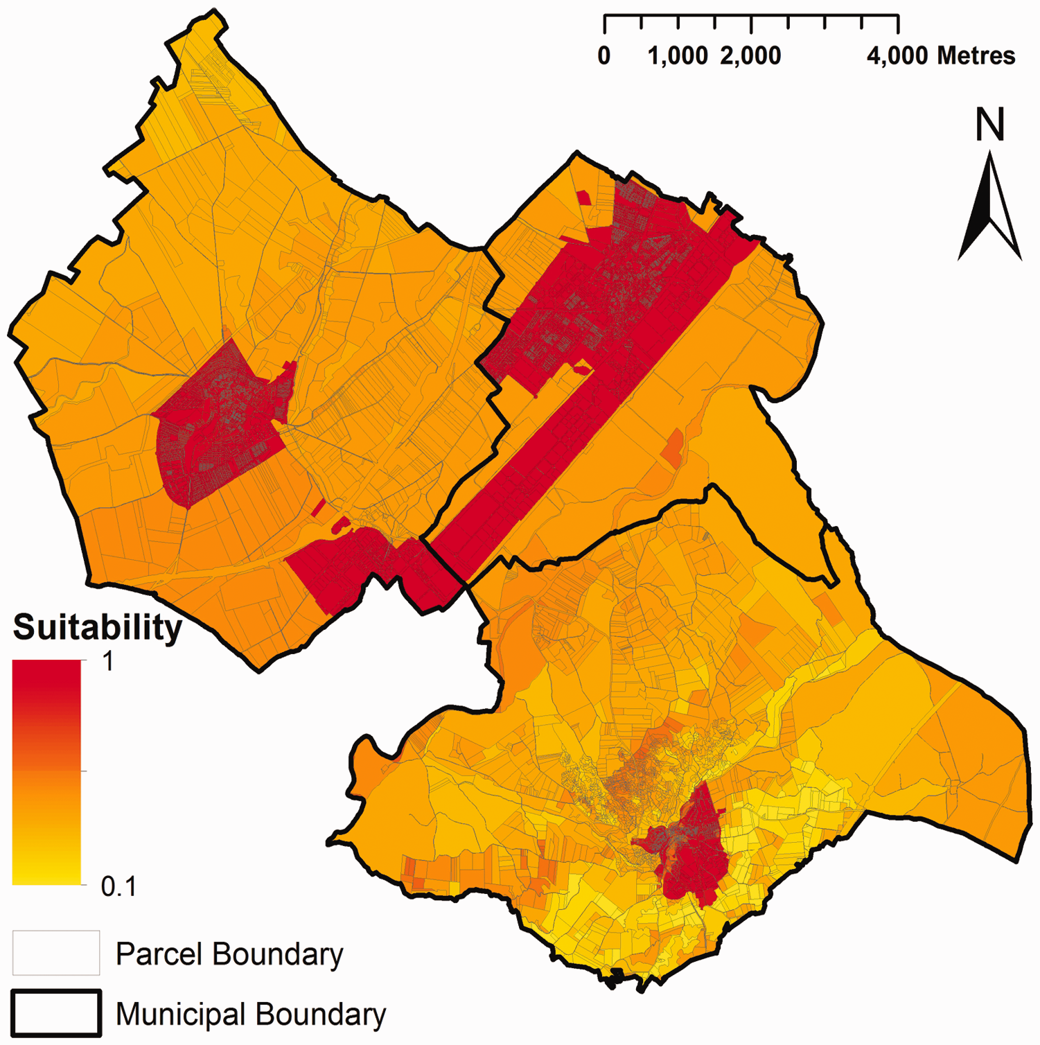
Suitability map.

Figure 5.

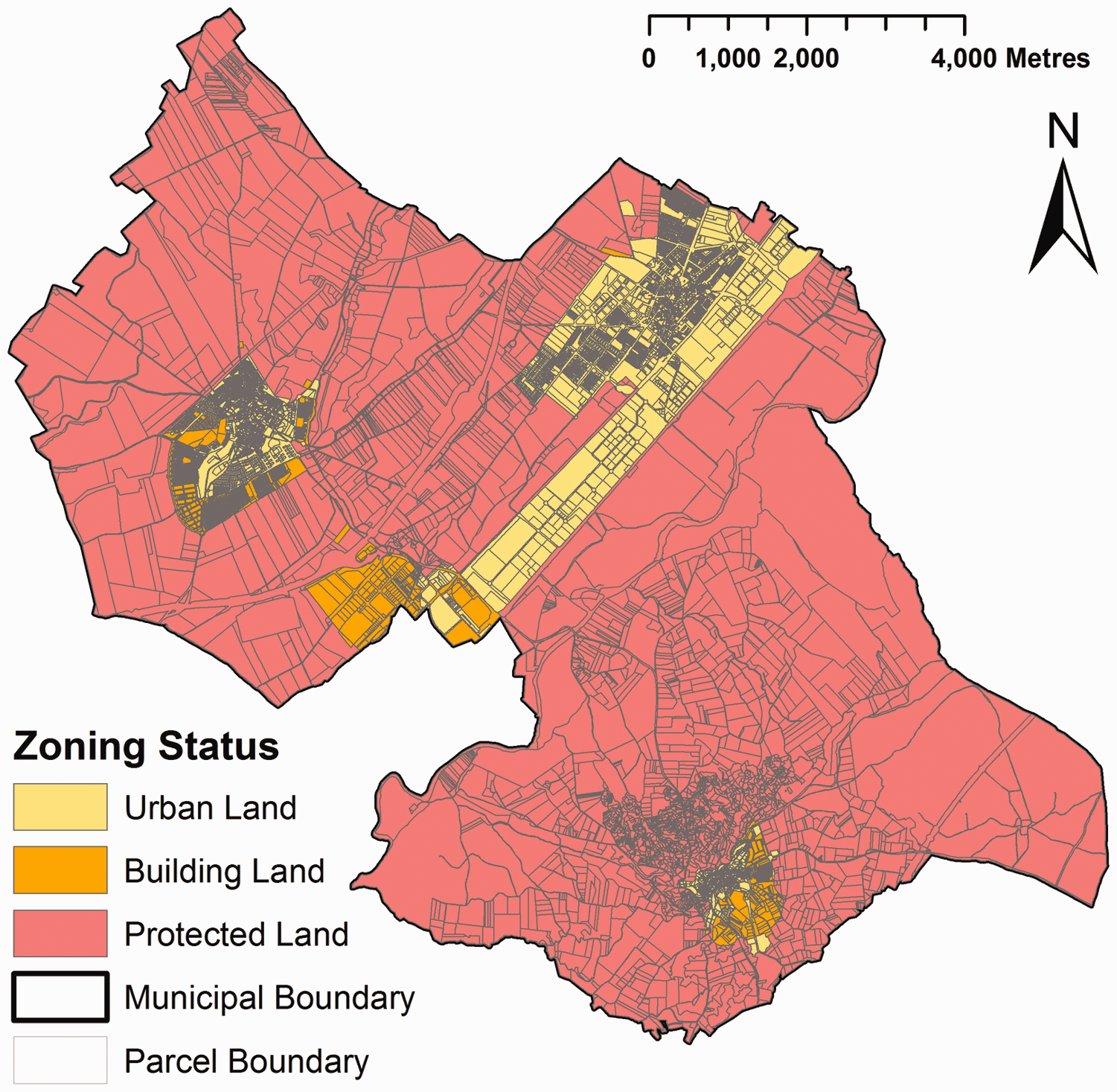
Zoning status map.

Zoning status

The land use zoning proposed in the urban plans of the three selected municipalities was used as the zoning status parameter. MUGICA assigned the real zoning status to all parcels included in the study area without the need to rasterise the map. Parcels were included or excluded as vacant land in each model run depending on their zoning status (Figure 5).

Random factor

Urban processes at very detailed scales do not always correspond to deterministic causes and present a certain degree of randomness (García et al., 2011). Consequently, CA-based models usually incorporate a component of randomness. CA-based models commonly calculate the potential value to develop an urban land use by combining NASZ values for each cell or parcel. This potential value is then modified by using a random component that introduces a perturbation of the value (White and Engelen, 1993), or by using the Monte Carlo method, whereby the potential value is compared with a random number to decide on development (De Almeida et al., 2003; Wu, 2002). This kind of perturbation is commonly known in the literature as the stochastic disturbance and it was incorporated into the MUGICA model using equation (2)

R = 1 + (- Inrand)^{α}

(2)

where R is the stochastic disturbance, rand is a random number between 0 and 1 and α is a number that controls the size of the disturbance. This exponent was tested for values between 0.1 and 1 in steps of 0.1.

A second component was added to the random factor in MUGICA to reflect the Spanish context. During the housing bubble in Spain (1997–2008), certain parcels developed a residential or productive land use even though they were zoned as protected or non-building land (Burriel, 2011). This phenomenon has been explored by other authors in other countries (e.g. Alfasi et al., 2012; White et al., 2015). Hence, the aim of the second component, named Random Protected Land Development (RPLD), was to add parcels with ‘protected land’ zoning status to the set of candidates to develop a new urban area, in order to simulate possible illegal growth. The amount of area added was based on the percentage of the detected area illegally developed in the region between 2000 and 2010 (14% for residential use and 25% for productive use).

Implementation of MUGICA

MUGICA is based on a previous prototype (Barreira-González et al., 2015a). The model uses a series of concatenated Python functions, enabling correct performance. The flowchart (as shown in Figure 6) can be divided into three independent but interconnected blocks.

Figure 6.

Model flowchart.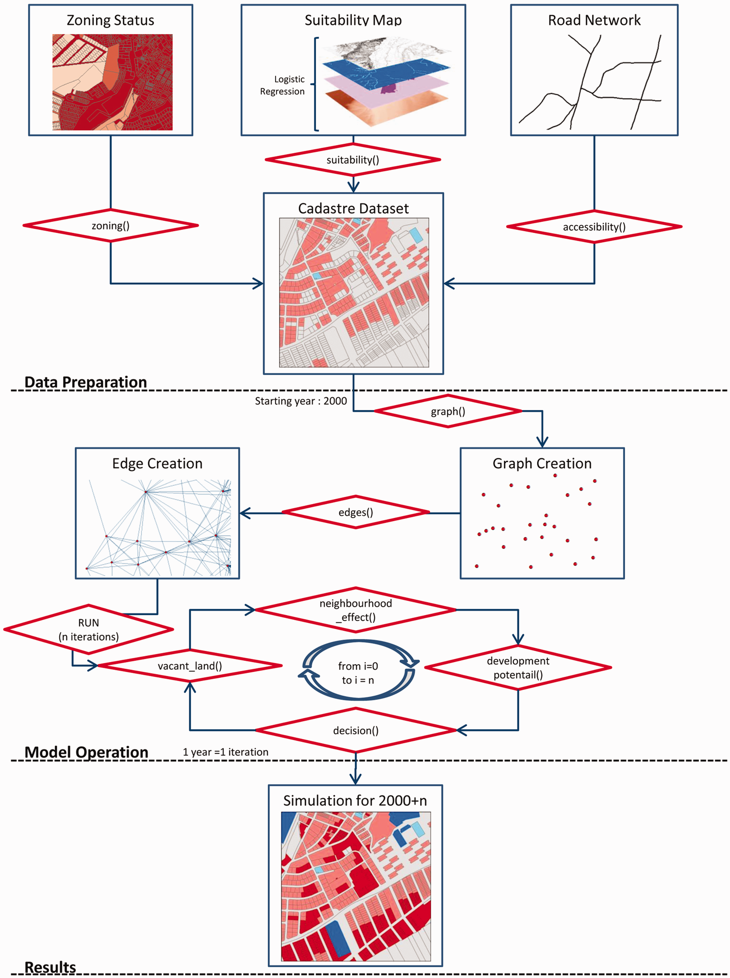

The first block prepares the data required during model operation. In this step, all the geospatial information is integrated: the suitability map is calculated, neighbourhood is defined, accessibility is measured and zoning status is added at parcel level.

The second block covers model operation, in which the information is abstracted onto a graph in order to reduce computational time (Barreira-González et al., 2015a). In this case, the graph nodes are the cadastre parcels, storing all the information relative to the parcel, and the connections between them are defined through the neighbourhood as described in the section entitled Neighbourhood.

Once the graph is fully completed, the model starts iterating, calculating the vacant land that is available to develop a new urban land use. Here, the RPLD component adds areas with protected land zoning status to vacant land. Two land uses are simulated: residential and productive (commercial and industrial). With the available land identified, the model calculates the neighbourhood effect for the first year, and then the equation of potential is applied (equation (3))

P_{i, k} = N_{i, k} \cdot A_{i} \cdot S_{i} \cdot Z_{i} + R

(3)

where k is the land use for parcel i, N is the neighbourhood effect to develop land use k, A is accessibility, S is suitability, Z is the zoning status and R is the stochastic disturbance.

For each parcel classified as vacant land, two values of potential are obtained: one to develop a residential land use and another to develop a productive land use. The model determines which is the highest and develops parcels until demand for each land use is fulfilled. Parcels that have developed new land uses during this iteration are updated in the graph and the new situation is introduced as the starting data for the next iteration. In this version of MUGICA, the model has no subdivision algorithm that divides large rural spaces into smaller parcels. The model works iteratively until the final year of simulation is reached (1 iteration corresponds to one calendar year). In addition, MUGICA does not consider transitions from urban land use to rural, since this is not a common occurrence in the study area or more generally in the rest of the country.

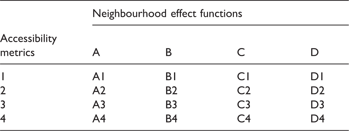
The last block transfers the results stored in the graph to the cadastre data set in order to obtain the spatial results. Using the same flowchart proposed in Figure 6, and in order to test model performance, a total of 224 versions of the MUGICA were produced under different combinations of different factor implementations: the four neighbourhood effect functions (A, B, C and D), the suitability map obtained through logistic regression, the four accessibility metrics (1, 2, 3 and 4) and the zoning status obtained for each parcel produced a total of 16 versions (Table 2), each of which in turn produced 14 more versions (224 in total) using 14 different neighbourhood distances, from 25 m to 500 m.

Table 2.

Notation for MUGICA versions.

	Neighbourhood effect functions
Accessibility metrics	A	B	C	D
1	A1	B1	C1	D1
2	A2	B2	C2	D2
3	A3	B3	C3	D3
4	A4	B4	C4	D4

Calibration: Simulation for 2000–2010 and accuracy assessment

To test the MUGICA model, it was necessary to study the random factor in isolation in order to understand how the rest of the factors contributed to the results (Barreira-González et al., 2015b). Thus, the model was first tested without randomness, running each of the 224 versions of MUGICA from 2000 to 2010 and comparing the results against observed growth for 2010. Then, the version that best reproduced urban growth for 2010 was selected and the random factor was introduced into that version of MUGICA to test its performance. The results for the versions of MUGICA without randomness are given in the section entitle Simulation for 2010 and selection of the optimum version of MUGICA.

Once the version of MUGICA with the best fit had been selected, another 10 versions of the model were produced, which included the RPLD and different stochastic disturbance sizes (R) using 10 different values for α, from 0.1 to 1.0 in steps of 0.1. These 10 versions were each run 100 times (1000 in total) in order to measure the variability of the results due to each stochastic disturbance size. The results for the versions of MUGICA that include randomness are given in the section entitled Incorporation of the random factor into the MUGICA version with the best fit.

A recurrent question when comparing model simulation results with observed changes or growth is how well the model performed (Pontius et al., 2008), or in other words, which is the best metric to determine agreement. In this study, we adapted the cross tabulation matrix usually employed in remote sensing to compare classified images against reality (Congalton and Green, 2008). As shown in Figure 7, the values in the matrix are not pixels, but parcel area. Producer accuracy (PA) was employed to determine the proportion of the simulation per land use that had been located correctly according to observed growth. A new metric called growth simulation accuracy (GSA) was developed. This metric aims to evaluate how well the model locates growth, independently of the land use simulated. For example, if residential growth was observed within a parcel, but the model simulates productive use, GSA will consider this fact an agreement since the metric measures the agreement between observed and simulated growth. GSA is expressed in a percentage form, so it can take values from 0% to 100%.

Figure 7.

Metrics derived from the cross tabulation matrix between simulated and observed growth.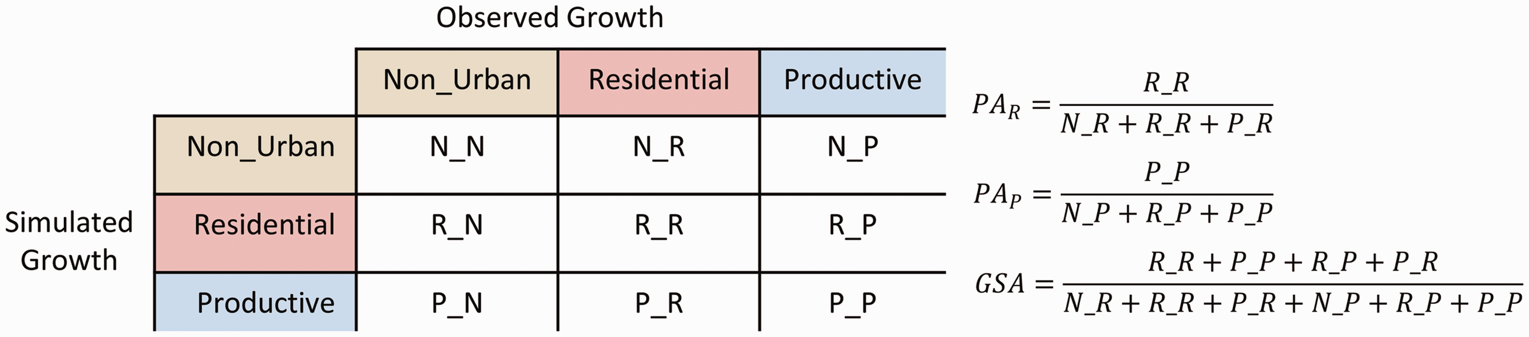

Results

Simulation for 2010 and selection of the optimum version of MUGICA

All versions of MUGICA (224) were run from 2000 to 2010 and then compared against observed growth for 2010. Figure 8 shows the results obtained for each comparison metric selected. The model version can be identified according to the notation shown in Table 2 and the neighbourhood definition distance shown in the x-axis.

Figure 8.

(a) Producer accuracy for residential land use. Values lower than 40% are not represented (accessibility metric 4). (b) Producer accuracy for productive land use. (c) Growth simulation accuracy.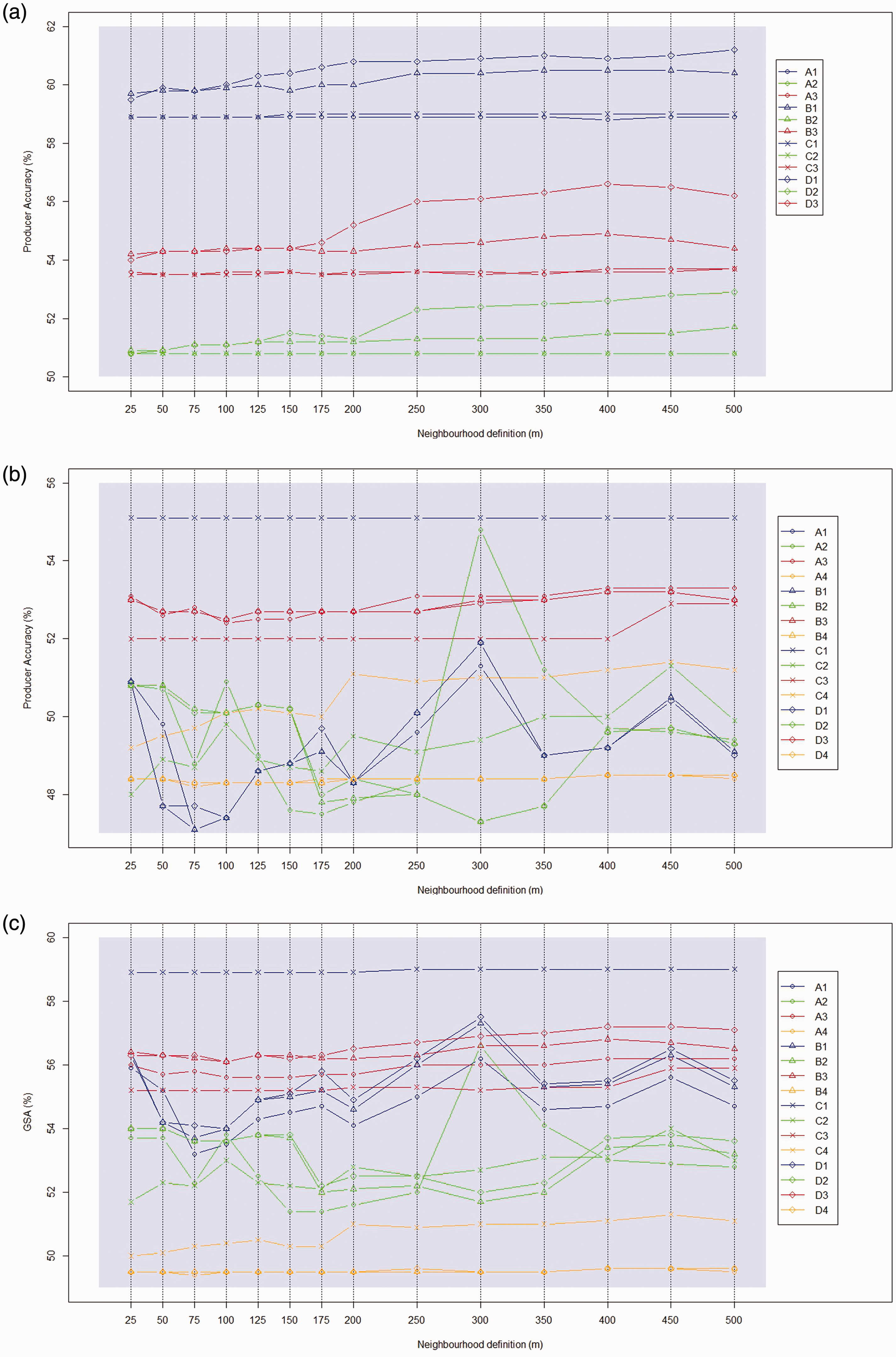

Figure 8(a) shows that when using the same accessibility metric, the results for residential land use presented similar PA values to the values grouped by colour. This may mean that the results obtained from MUGICA are highly sensitive to the selected set of functions that reproduce the neighbourhood effect. Thus, the results obtained with metric 1 (in blue) presented the highest PA values, which means that the version of MUGICA that employed this metric reproduced observed growth better than the other versions. In the case of the different neighbourhood effect functions, set D presented better results than the other sets when using the same neighbourhood distance and accessibility metric. The best simulated-observed residential agreement corresponded to D1, and this rose as neighbourhood distance increased.

In the case of productive land use (Figure 8(b)), the PA results were not analogous to those for residential land use. C1 best reproduced the observed productive growth, independently of the neighbourhood distance selected. The results seem to be similar in the case of accessibility metric 3 (A3, B3, C3 and D3), with small differences between them. The least homogeneous results were given by metric 2, which did not present a clearly recognisable pattern. Neighbourhood distance did not appear to generate higher or lower PA values when this parameter was modified in MUGICA for this land use, whereas the choice of accessibility metric in combination with the neighbourhood effect functions exerted a clear effect on the results.

An analysis of the results obtained from the different versions of MUGICA taking into account the location of the simulated growth, independently of the land use simulated (GSA), revealed a combination of factors that clearly obtained the best fit (Figure 8(c)). This was the C1 version of MUGICA, where neighbourhood distance was defined as 250 m, and this was used to test the random factor in the model. As it can be seen in the three Figure (8(a)–(c)), there are some factor combinations that show constant lines (horizontal), which mean that their results of PA or GSA do not vary according to neighbourhood distance definition. This fact implies that in some cases, the use of large distances should raise these values, but it is not the case. Further research is needed in order to clarify if the nature of the study area is affecting these results.

Incorporation of the random factor into the MUGICA version with the best fit

RPLD and R were incorporated into the MUGICA version with the best fit, and this was run 1000 times: 100 times per different stochastic disturbance value (from 0.1 to 1). Bean plots in Figure 9 show the GSA metric results obtained for the simulations. Only GSA was used since the aim was to determine which combination best reproduced urban growth, without considering land use.

Figure 9.

Growth simulation accuracy for MUGICA version C1, 250 m.

The x-axis shows all values for α. The black line in each bean represents the mean GSA for the 100 simulations of each version, and the width of the bean represents the frequency of the results. The highest GSA was obtained for α = 0.4, although the adjacent values of 0.3 and 0.5 presented similar results. The shape of the bean, close to the shape of a rhombus, suggests that the results presented a normal distribution, which was the case of 0.4. Thinner beans indicate that the results were more dispersed, with high variability due to the size of stochastic disturbance selected. In the case of 0.4, GSA values ranged from 65% to 50%. Thus, the implemented random factor modified the model results by ± 7.5%.

Spatial results

The spatial results obtained from the simulations performed with the C1 MUGICA model are shown in Figure 10. Figure 10(a) represents the 100 simulations of the version with the best fit and using α = 0.4, providing the cartography of the parcels most repeatedly simulated by the model (Barreira-González et al., 2015b; Brown et al., 2005). As can be seen, parcels with deep red represent locations that were selected by the model in over 80% of the simulations.

Figure 10.

(a) Frequency map of parcels developed after running 100 simulations of MUGICA C1 with α = 0.4. (b) Best-fit simulation compared to observed growth.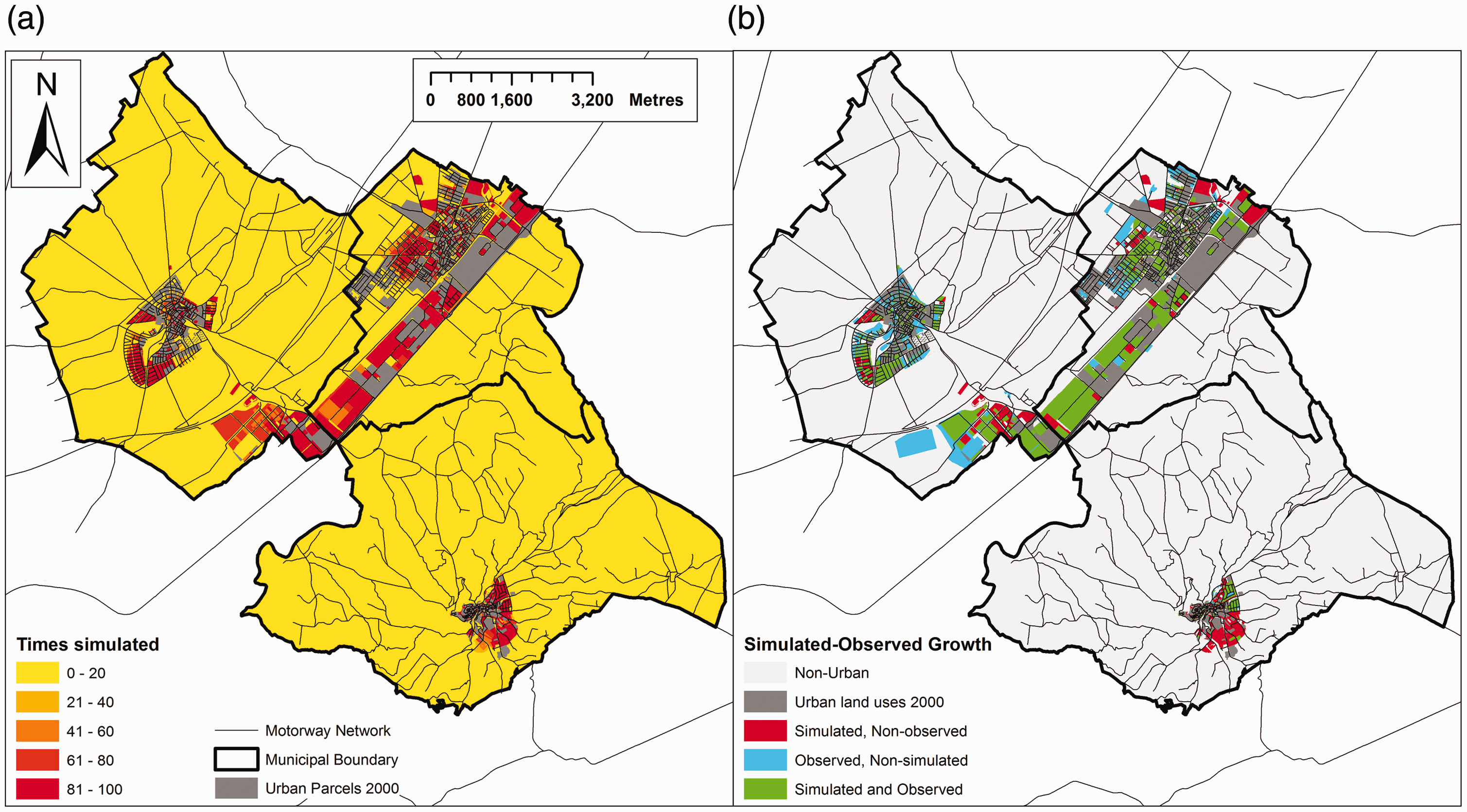

Figure 10(b) represents the agreement with observed growth for the best of the 100 simulations carried out. Parcels in green represent those areas where the model correctly simulated the observed growth between 2000 and 2010, which also appear in the numerator of GSA equation. These parcels are mainly located along the motorway corridor or in certain locations close to the urban centres of the three municipalities. Parcels in blue represent model errors of omission: parcels where urban growth occurred but the model did not simulate it. Parcels in red represent errors of commission: parcels where urban growth did not occur but where this was simulated by the model.

Discussion and conclusions

MUGICA has demonstrated the capacity to reproduce the principles of classical CA-based models but in an irregular environment using cadastral parcels. The use of this structure required a redefinition of the different factors included in typical CA-based models that simulate urban growth. Calibration of these factors has been assessed through a sensitivity analysis, testing the extent to which the results obtained from the model are sensitive to changes in each of the factors implemented (Barreira-González et al., 2015b).

In line with the methodology proposed by Barreira-González and Barros (2017), several neighbourhood definition distances were used to obtain a function of effect for each land use and spatial metric. The GSA results show that selecting a different neighbourhood distance did not influence the results, with differences of less than 4% when using the same neighbourhood effect function and accessibility metric. Nevertheless, the global results obtained over 55% for GSA for most versions of MUGICA. This finding contrasts with the results obtained in other studies that have analysed the variation in results in relation to neighbourhood distances in regular CA-based models (Jantz and Goetz, 2005; Kocabas and Dragicevic, 2006) or irregular ones (Barreira-González and Barros, 2017). The inclusion of more land uses might lead to an increase in the differences, but further research is required in order to assess this issue.

The accessibility metrics proposed here, which constitute a new approach to the concept of accessibility with respect to traditional CAs, have demonstrated their capacity to characterise ease of access from a parcel to given elements. The metrics (1 and 2) that employ distances to measure accessibility seem to be more effective, obtaining higher PA and GSA values than those that employ time (3 and 4). These results are evidently sensitive to changes in the target locations selected (Handy and Niemeier, 1997), and therefore further investigation using several sets of locations would complement the study.

Regarding the random factor, a new alternative has been proposed to address the uncertainty that complex processes such as urban growth entail (García et al., 2011). The RPLD component more realistically represents the dynamic experienced in the Spanish context, where there has been illegal growth in recent decades. In this sense, there is a need to evaluate how the development potential of each parcel evolves during model operation to test the extent of the influence of stochastic disturbance and RPLD. Other methods that have been explored in this field, such as the Monte Carlo method (Wu, 2002), may contribute to improving the R component.

Urban plans depict the zoning status of every area using the smallest spatial unit in planning: parcels. Thus, zoning is defined at the parcel level. Implementation of this factor enables the future inclusion of planning modifications to simulate scenarios within MUGICA. The model has the capacity to integrate all the information for each factor at parcel level for later on, transferring the information to a graph. The simple structure of graphs consistently reduces the computational time required to run the model and preserves the spatial structure as well as maintaining the neighbourhood definition. These advantages render this structure more promising for inclusion in irregular CA-based modelling.

MUGICA accurately locates past urban growth, with over 60% agreement. Some authors have tended to include stable areas in their calculation of agreement, increasing their values of coincidence from 70% to over 90% (Barredo et al., 2004; Moreno et al., 2009, Pinto and Antunes, 2010). In the case of MUGICA, stable areas were not included in the calculation of GSA or PA, in order to highlight the correct performance of the model.

The irregular structure employed here presents several advantages, such as using a more realistic spatial unit rather than regular grids or pixels (Zelaya et al., 2016). In this regard, the cadastral parcel is the smallest unit employed in planning, and as indicated by Triantakonstantis and Mountrakis (2012), the use of the same spatial structure as that employed by planners may be necessary in order to include models in the planning process. We believe that the use of this structure renders models more comprehensible and more likely to be used by planners. In addition, the results obtained from simulations could be employed in workshops with agents to move planning processes forwards based on participatory scenarios. As shown in Figure 10(a), identification of the parcels that are most repeatedly simulated by the model could be useful to planners using this kind of model (Barreira-González et al., 2015b), and would contribute to better-founded discussion.

However, the use of cadastre parcels also presents some drawbacks. The main one is related to large parcels. Traditionally, parcels in rural areas have tended to be much larger than those located in urban areas. When these large parcels are developed, they are not usually developed as a whole, but rather tend to be subdivided. The current MUGICA version does not have the capacity to divide them into several smaller units. A subdivision algorithm is thus required to complement the other elements used in the model, as well as testing more land uses in the urban environment.

A map comparison of simulated and observed growth is a key question in calibration and validation processes. Here, we have proposed an adaptation of the traditional cross tabulation or confusion matrix with PA and GSA metrics to provide an accurate indication of how well the model is performing. Although the above-mentioned metrics considered the spatial location of the results, there is also a need to explore spatial metrics (Herold et al, 2003) in order to analyse the results in terms of fragmentation and dispersion (Barreira-González et al 2015b). Another approach could be to adapt moving window metrics (Soria-Lara et al, 2016) to irregular environments.

Footnotes

Declaration of conflicting interests

The author(s) declared no potential conflicts of interest with respect to the research, authorship, and/or publication of this article.

Funding

The author(s) disclosed receipt of the following financial support for the research, authorship, and/or publication of this article: This research was performed as part of the SIMURBAN2 project (Geosimulation and environmental planning in metropolitan spatial decision making. Implementation at intermediate scales) (CSO2012-38158-C02-01), funded by the Spanish Ministry of Economy and Competitiveness. The University of Alcalá supports the first author within the “Ayudas para la Formación de Personal Investigador (FPI) 2012” framework.

Pablo Barreira-González is engineer in Geodesy and Cartography, holds a MSc in geographical information technologies and is a PhD student. He is researcher personnel at the University of Alcalá, Spain, where he helps in teaching subjects related to GIS, programming and cartography. His main research is focused on urban growth simulation models and map comparison methods, among others.

Francisco Aguilera-Benavente holds a BSc in environmental sciences and a PhD in geographical information technology. He is associate professor of human geography at the University of Alcalá, Spain, where he teaches several subjects related to GIS and spatial analysis. Urban growth simulation models and urban growth patterns analysis are among his main research topics.

Montserrat Gómez-Delgado is a geographer that holds a PhD in geographical information technologies. She is lecturer in human geography at the University of Alcalá, Spain, where she teaches several subjects related to GIS and human geography. Her main research interests focus on urban growth simulation models and validation procedures among others.

References

Aguilera

Valenzuela

Bosque

(2010) Simulación de escenarios futuros en la aglomeración urbana de granada a través de modelos basados en autómatas celulares. Boletín De La Asociación De Geógrafos Españoles 54: 271–300.

Alfasi

Almagor

Benenson

(2012) The actual impact of comprehensive land-use plans: Insights from high resolution observations. Land Use Policy 29(4): 862–877.

Arsanjani

Helbich

Kainz

et al. (2013) Integration of logistic regression, Markov chain and cellular automata models to simulate urban expansion. International Journal of Applied Earth Observation and Geoinformation 21: 265–275.

Barredo

Demicheli

Lavalle

et al. (2004) Modelling future urban scenarios in developing countries: An application case study in Lagos, Nigeria. Environment and Planning B: Planning and Design 31(1): 65–84.

Barredo

Kasanko

McCormick

et al. (2003) Modelling dynamic spatial processes: Simulation of urban future scenarios through cellular automata. Landscape and Urban Planning 64(3): 145–160.

Barreira-González

Aguilera-Benavente

Gómez-Delgado

(2015b) Partial validation of cellular automata based model simulations of urban growth: An approach to assessing factor influence using spatial methods. Environmental Modelling and Software 69: 77–89.

Barreira-González

Barros

(2017) Configuring the neighbourhood effect in irregular cellular automata based models. International Journal of Geographical Information Science 31(3): 617–636.

Barreira-González

Gómez-Delgado

Aguilera-Benavente

(2015a) From raster to vector cellular automata models: A new approach to simulate urban growth with the help of graph theory. Computers, Environment and Urban Systems 54: 119–131.

Bavoux

Beaucire

Chapelon

et al. (2005) Géographie des transports, Paris: Armand Colin.

10.

Bengston

Fletcher

Nelson

(2004) Public policies for managing urban growth and protecting open space: Policy instruments and lessons learned in the United States. Landscape and Urban Planning 69(2): 271–286.

11.

Brown

Page

Riolo

et al. (2005) Path dependence and the validation of agent-based spatial models of land use. International Journal of Geographical Information Science 19(2): 153–174.

12.

Burriel

(2011) Subversion of land-use plans and the housing bubble in Spain. Urban Research and Practice 4(3): 232–249.

13.

Congalton

Green

(2008) Assessing the Accuracy of Remotely Sensed Data: Principles and Practices, Boca Ratón: CRC press.

14.

Couclelis

(1997) From cellular automata to urban models: New principles for model development and implementation. Environment and Planning B: Planning and Design 24: 165–174.

15.

Dahal

Chow

(2014) An agent-integrated irregular automata model of urban land-use dynamics. International Journal of Geographical Information Science 28(11): 2281–2303.

16.

Dahal

Chow

(2015) Characterization of neighborhood sensitivity of an irregular cellular automata model of urban growth. International Journal of Geographical Information Science 29(3): 475–497.

17.

De Almeida

Batty

Monteiro

AMV

et al. (2003) Stochastic cellular automata modeling of urban land use dynamics: Empirical development and estimation. Computers, Environment and Urban Systems 27(5): 481–509.

18.

Fundation OSG (2008) GDAL-OGR: Geospatial Data Abstraction Library/Simple Features Library Software. Available at: http://gdal.osgeo.org.

19.

García

Santé

Crecente

et al. (2011) An analysis of the effect of the stochastic component of urban cellular automata models. Computers Environment and Urban Systems 35: 289–296.

20.

García

Santé

Boullón

et al. (2012) A comparative analysis of cellular automata models for simulation of small urban areas in Galicia, NW Spain. Computers, Environment and Urban Systems 36(4): 291–301.

21.

Gardner

(1970) Mathematical games: The fantastic combinations of John Conway’s new solitaire game “life”. Scientific American 223(4): 120–123.

22.

General Directorate for Cadastre (2013) Ministry of Finance and Public Administration, Government of Spain. Available at: http://www.catastro.meh.es/ (accessed 15 October 2013).

23.

Gutiérrez

(2009) Transport and accessibility. International Encyclopedia of Human Geography 1: 410–417.

24.

Handy

Niemeier

(1997) Measuring accessibility: An exploration of issues and alternatives. Environment and Planning A 29(7): 1175–1194.

25.

Hansen

(2012) Empirically derived neighbourhood rules for urban land-use modelling. Environment and Planning B: Planning and Design 39(2): 213–228.

26.

Herold

Couclelis

Clarke

(2005) The role of spatial metrics in the analysis and modeling of urban land use change. Computers, Environment and Urban Systems 29(4): 369–399.

27.

Herold

Goldstein

Clarke

(2003) The spatiotemporal form of urban growth: Measurement, analysis and modeling. Remote Sensing of Environment 86(3): 286–302.

28.

Hewitt

Escobar

(2011) The territorial dynamics of fast-growing regions: Unsustainable land use change and future policy challenges in Madrid, Spain. Applied Geography 31(2): 650–667.

29.

Jantz

Goetz

(2005) Analysis of scale dependencies in an urban land-use-change model. International Journal of Geographical Information Science 19: 217–241.

30.

Kocabas

Dragicevic

(2006) Assessing cellular automata model behaviour using a sensitivity analysis approach. Computers, Environment and Urban Systems 30(6): 921–953.

31.

Lau

Kam

(2005) A cellular automata model for urban land-use simulation. Environment and Planning B: Planning and Design 32(2): 247–263.

32.

Yeh

AGO

(2000) Modelling sustainable urban development by the integration of constrained cellular automata and GIS. International Journal of Geographical Information Science 14(2): 131–152.

33.

Martín-Varés

(2009) La importancia de llamarse Parcela Catastral. CT: Catastro 66: 7–24.

34.

Moreno

Ménard

Marceau

(2008) VecGCA: A vector-based geographic cellular automata model allowing geometric transformations of objects. Environment and Planning B: Planning and Design 35(4): 647–665.

35.

Moreno

Wang

Marceau

(2009) Implementation of a dynamic neighborhood in a land-use vector-based cellular automata. Computers Environment and Urban Systems 33: 44–54.

36.

NOMECALLES Nomenclátor Oficial y Callejero (2016) Comunidad de Madrid, Consejería de Economía e Innovación Tecnológica. Instituto de Estadística. Available at: http://www.madrid.org/nomecalles (accessed 1 February 2016).

37.

O’Sullivan

(2001) Graph-cellular automata: A generalised discrete urban and regional model. Environment and Planning B: Planning and Design 28: 687–706.

38.

Pinto

Antunes

(2010) A cellular automata model based on irregular cells: Application to small urban areas. Environment and Planning B-Planning and Design 37: 1095–1114.

39.

Plata Rocha

Gómez Delgado

Bosque Sendra

(2009) Cambios de usos del suelo y expansión urbana en la Comunidad de Madrid (1990-2000). Scripta Nova: revista electrónica de geografía y ciencias sociales 293(13): 27 pages online.

40.

Pontius

Jr Boersma

Castella

et al. (2008) Comparing the input, output, and validation maps for several models of land change. The Annals of Regional Science 42(1): 11–37.

41.

R Core Team (2013) R: A language and environment for statistical computing. Vienna, Austria: the R Foundation for Statistical Computing. ISBN: 3-900051-07-0. Available at: http://www.R-project.org/.

42.

Sakieh

Amiri

Danekar

et al. (2015) Simulating urban expansion and scenario prediction using a cellular automata urban growth model, SLEUTH, through a case study of Karaj City, Iran. Journal of Housing and the Built Environment 30(4): 591–611.

43.

Santé

Garcia

Miranda

et al. (2010) Cellular automata models for the simulation of real-world urban processes: A review and analysis. Landscape and Urban Planning 96: 108–122.

44.

Soria-Lara

Aguilera-Benavente

Arranz-López

(2016) Integrating land use and transport practice through spatial metrics. Transportation Research Part A: Policy and Practice 91: 330–345.

45.

Stevens

Dragicevic

(2007) A GIS-based irregular cellular automata model of land-use change. Environment and Planning B-Planning and Design 34: 708–724.

46.

Stevens

Dragicevic

Rothley

(2007) iCity: A GIS-CA modelling tool for urban planning and decision making. Environmental Modelling and Software 22(6): 761–773.

47.

Tobler

(1970) Computer movie simulating urban growth in Detroit region. Economic Geography 46: 234–240.

48.

Tobler W (1979) Cellular geography. In Philosophy in Geography Dordrecht: Reidel, Vol 20: pp. 379–386. ISBN: 978-94-009-9396-9.

49.

Triantakonstantis

Mountrakis

(2012) Urban growth prediction: A review of computational models and human perceptions. Journal of Geographic Information System 4(6): 555–587.

50.

United Nations (2014) World urbanization prospects: The 2014 revision, highlights. Department of Economic and Social Affairs. Population Division, United Nations. ISBN: 978-92-1-151517-6.

51.

Vandenbulcke

Steenberghen

Thomas

(2009) Mapping accessibility in Belgium: A tool for land-use and transport planning. Journal of Transport Geography 17(1): 39–53.

52.

Van Rossum G (2007) Python programming language. In USENIX Annual Technical Conference Santa Clara CA, USA 17–22 June 2007.

53.

Verburg

de Nijs

van Eck

et al. (2004) A method to analyse neighbourhood characteristics of land use patterns. Computers, Environment and Urban Systems 28(6): 667–690.

54.

Vickerman

(1974) Accessibility, attraction, and potential: A review of some concepts and their use in determining mobility. Environment and Planning A 6(6): 675–691.

55.

Wegener

(2004) Overview of land-use transport models. Handbook of Transport Geography and Spatial Systems 5: 127–146.

56.

White

Engelen

(1993) Cellular automata and fractal urban form: A cellular modelling approach to the evolution of urban land-use patterns. Environment and Planning A 25(8): 1175–1199.

57.

White

Engelen

Uljee

(1997) The use of constrained cellular automata for high-resolution modelling of urban land-use dynamics. Environment and Planning B: Planning and Design 24(3): 323–343.

58.

White R, Engelen G and Uljee I (2015) Modeling Cities and Regions as Complex Systems: From Theory to Planning Applications. Cambridge MA, USA and London, England: MIT Press. ISBN: 978-0-262-02956-8.

59.

(2002) Calibration of stochastic cellular automata: The application to rural-urban land conversions. International Journal of Geographical Information Science 16: 795–818.

60.

Zelaya

Van Vliet

Verburg

(2016) Characterization and analysis of farm system changes in the Mar Chiquita basin, Argentina. Applied Geography 68: 95–103.