A multiobjective optimization model for locating affordable housing investments while maximizing accessibility to jobs by public transportation

Abstract

This paper develops a new optimal location model for siting affordable housing units to maximize the accessibility of low-income workers to appropriate jobs by public transportation. Transit-accessible housing allows disadvantaged populations to reduce their reliance on automobiles, which can lead to savings on transportation-related expenditures. The housing location model developed here maximizes transit accessibility while reducing the clustering of affordable housing units in space. Accessibility is maximized using a high-resolution space-time metric of public transit accessibility, originally developed for service equity analysis. The second objective disperses subsidized housing projects across space using a new minimax dispersion model based on spatial interaction principles. The multiobjective model trades off accessibility maximization and affordable housing dispersion, subject to upper and lower bounds on the land acquisition and construction budget. The model is tested using data for Tempe, AZ including actual data for vacant parcels, travel times by light rail and bus, and the location of low-wage jobs. This model or similar variants could provide insightful spatial decision support to affordable-housing providers or tax-credit administrators, facilitating the design of flexible strategies that address multiple social goals.

Keywords

Affordable housing accessibility optimization location facility dispersion

Introduction

Providing decent housing affordable to persons and families of modest means has long been a goal of US housing policy (Schwartz, 2010). Additionally, families of all income levels require shelter and benefit from the private space that housing provides. The location of housing largely determines one's access to jobs, food, shopping, and opportunities for social interaction. In the US, affordable housing is often defined as housing for which the mortgage or rent does not exceed 30% of household income (US Department of Housing and Urban Development, 2015). When households can reasonably afford housing, they are less pressured to move when their budgets are strained and can maintain their location, neighborhood and social networks over longer periods. Prior work has shown that children in stable housing perform better in school and are less likely to experience disruption in their education (Cutuli et al., 2013; Rafferty et al., 2004). Affordable housing also reduces exposure to stress, toxins and infectious disease by alleviating crowding, which leads to better physical and mental health (Housingpolicy.org, 2016; Lubell et al., 2007).

Explicit policies aimed at achieving affordable housing generally operate in two basic ways: first, by providing subsidy vouchers households can use towards the rent in any unit, and second, by providing specific units which are designated to be affordable with specific rents depending on household sizes (which can be found within a building with market-rate units or in separate structures or developments containing only affordable units) (Schwartz, 2010). This paper introduces a technique to determine the location of the latter – housing units specifically produced to be affordable, often by a public housing authority or by the private sector with subsidies from public funds (e.g. tax credits).

Practitioners and scholars recognize that where affordable housing is sited is a significant factor in its success (Schwartz, 2010). Low-income workers, who provide essential services in their communities, often cannot afford to live in the communities they serve (Benner and Karner, 2016). Providing accessibility to jobs for low-income workers enhances social benefits and community equity. Proximity to jobs, shopping, transportation infrastructure, childcare, good public schools, parks, cultural activities, health facilities, counseling, and other supportive services benefit the occupants of affordable housing (Schwartz, 2010). Good site planning for affordable housing should therefore consider various scales – from adjacent buildings and neighborhoods to the entire metropolitan region.

Although it is acknowledged that location and accessibility are important ingredients in successful affordable housing, surprisingly little research has been undertaken to date to determine optimal investment locations. Yet the affordable housing location problem contains many of the themes found in other branches of facility location modeling: choosing a combination of locations from a set of candidate sites, maximizing access via existing networks, dealing with budget constraints, trading off efficiency and equity, and so on. The literature to date has focused heavily on two general factors. First, models usually maximize some measure of net economic or social benefit to the residents of the affordable housing or to the community or society. Second, some type of dispersion measure to reflect the “fair distribution” of affordable housing is usually incorporated to spread the impact of affordable housing across host communities.

This paper proposes new approaches to modeling each of these general siting factors. For maximizing social benefit, the proposed model focuses specifically on accessibility to job opportunities for low-wage workers by public transportation. The objective function incorporates a new public transit accessibility metric considering both the travel time of both the transit trip and the first and last mile access to transit stops, as well as the number and type of jobs. For equitable impact, the model proposes a modified facility dispersion function that takes into account traditional spatial interaction factors such as facility size and separation distance embedded in a new minimax formulation. The resulting multiobjective model locates affordable housing facilities of different sizes to maximize accessibility by residents to low-wage jobs by public transportation and minimize the maximum dual impact of affordable housing developments located close to each other. Model outputs could be used to narrow down the universe of all possible combinations of affordable housing sites to a small set of Pareto-optimal solutions on a tradeoff frontier between these two objectives.

The data inputs to the model take into account the location, size, and zoning of vacant land parcels, suitable job availability, public transportation routes and access to these routes, land and constructions costs, the affordable housing construction budget. Our model does not take into account the political or geographical environment in which affordable housing is located within a region – i.e. whether such housing is steered into certain areas or in some other way constrained.¹ Similarly, we do not connect the model explicitly to a process of housing advocacy or decision-making beyond the specific case developed here, though this model could clearly feed into a broader process of regional housing advocacy or planning in a “community operations research” context (e.g. Midgley and Ochoa-Arias, 2004).

The next section reviews prior work on optimization models for affordable housing, accessibility metric calculation methods, and dispersion models for creating equitable distribution of facilities. We subsequently discuss the methods and data underlying our affordable housing location optimization model before describing the case study location of Tempe, Arizona, USA. The paper concludes with a discussion of the model results and potential next steps.

Literature review

Optimization models for location of affordable housing

Very few optimization models have been specifically designed for locating affordable or subsidized housing. Some of the earliest operations research work on housing includes two papers on tenant assignment models for relocation of households from public housing during renovations (Kaplan, 1986; Kaplan and Berman, 1988). Later work developed decision support tools for the US Army for locating new military housing units and determining whether to construct or lease housing on-base or off (Forgionne, 1991, 1997; Forgionne and Frager, 1998). Since 2000, Michael P. Johnson and his co-authors have published most of the optimal affordable housing location papers.

This literature can be categorized in several ways, such as by type of housing assistance. It began with the location of rent-subsidized housing (Johnson and Hurter, 1998) and progressed to tenant-based programs for relocation of households from inner-city public housing to Section 8 housing in less-disadvantaged neighborhoods (Johnson, 2003; Johnson and Hurter, 2000; Johnson et al., 2002) and project-based programs for lower-density subsidized housing. Johnson (2007) developed a two-stage approach in which the first stage is a strategic knapsack-type model for choosing how to allocate a given amount of funding across different housing programs. The second-stage model optimizes the locations and sizes of the affordable housing complexes within those programs. After the late-2000s recession, Johnson et al. (2010) and Bayram et al. (2011) optimized acquisition of foreclosed housing to stabilize vulnerable neighborhoods while providing affordable housing. Johnson et al. (2014) used a multiobjective model for allocating vacant land to residential and non-residential purposes. In addition to Johnson's group, Zhang et al. collaborated on two papers using a GIS-based spatial decision support system for public affordable housing (Zhang et al., 2009, 2013).

The work by Johnson and co-authors has largely defined the direction of this research subfield which uses multiobjective programming to trade off or balance (a) the beneficial impacts to residents of the facilities and (b) fairness concerns regarding perceived negative impacts on host communities with high concentrations of affordable housing. These two general objectives have taken a number of different forms. Johnson and Hurter (1998) incorporated many different kinds of benefits related to market rents, entry-level employment, and distance between origin and destination locations for families. From there, the literature moved towards net social benefit objective functions based on consumer surplus functions. Examples of factors considered include: income differences between residents of different types of public housing; operating subsidies required to provide affordable housing; and negative effect of public housing on surrounding property values (Johnson, 2003, 2006, 2007; Johnson and Hurter, 2000). Rent subsidies have been considered as an upper bound on the dollar value of the family benefit of living in a “better” neighborhood.

In this affordable housing optimization literature, the measures of benefits to programs participants are generally traded off against perceived fairness or equity to the host communities. Whether or not there are actual disbenefits from introducing lower-income families into higher income neighborhoods, there can be political opposition to public housing in neighborhoods based on the perception of negative impacts (Nguyen, 2005; Tighe, 2010). Therefore, any optimization of housing location would need to recognize this political reality and attempt to disperse in some manner the perceived “burdens” of affordable housing location (Johnson, 2003). These papers frame this second objective in terms of “distributional inequity,” which is operationalized as making the worst case of some particular metric as good as possible. Some of the papers minimize the maximum disparity between a neighborhood's proportion of total population and its proportion of public housing (Johnson, 2003; Johnson and Hurter, 2000). If one neighborhood has a substantially higher share of affordable housing than any other in the model, the model will shift housing to other neighborhoods. Other papers used a p-dispersion objective (Kuby, 1987) to maximize the minimum distance between the closest pair of affordable housing locations (Johnson, 2006). An advantage of the p-dispersion objective is that it does not depend on neighborhood boundaries. A disadvantage is that the objective ignores the size of the facilities and total number of other facilities that may be impacting a neighborhood. Johnson et al. (2010) employed a maxisum dispersion model, which maximizes the sum of each location's closest other location rather than the single worst-case closest pair. Kuby (1987) originally showed that the maxisum objective tends to produce clusters of facilities maximally dispersed from other clusters, which Johnson, Turcotte, and Sullivan adopted because it spreads facilities out while recognizing that it is more efficient for housing managers to manage units that are grouped near to other units.

Accessibility metrics and affordable housing

While the importance of public transportation to residents of affordable housing is well understood and has been incorporated into GIS models (Zhang et al., 2009, 2013), prior optimization models have not accounted explicitly for job accessibility by public transportation. Accessibility refers to the ease with which destinations can be reached given a particular configuration of the land use and transportation system (Geurs and van Wee, 2004; Handy and Niemeier, 1997). Accessibility can be increased either by locating origins and destinations close together or by decreasing the travel time between them. Commonly employed accessibility metrics include: cumulative opportunities measures that count all available opportunities located within a specified time threshold (e.g. 30 or 45 minutes of travel time); gravity measures that weight nearby opportunities more heavily; competitive accessibility measures that consider the number of people in competition for a given set of opportunities (jobs); or logsum measures derived from discrete choice models that are based on the utility of a given set of modes and travel times for a particular origin-destination pair. Each of these types of measures has been widely applied (Golub and Martens, 2014; Golub et al., 2013; Paez et al., 2010; Shen, 1998, 2001).

Accessibility calculations are fundamentally based upon travel times between origins and destinations and counts of opportunities available throughout a region. Travel times can reflect non-motorized travel, public transit use, or automobiles. Much of the literature on accessibility has had to rely on travel demand modeling skims derived from regional models. These skims describe travel times between transportation analysis zone (TAZ) centroids. While TAZ–TAZ travel times might work well for estimating travel time by automobile, they are too spatially coarse for modeling public transit. Because transit is often accessed via walking at the origin and destination end, and because destinations are not uniformly distributed across a TAZ, understanding the precise configuration of the pedestrian network in relation to opportunity locations is vital for understanding public transit accessibility. Software tools are now available that facilitate the type of spatial and temporal resolution required for a robust assessment of public transit accessibility and these have seen increasing application in the literature (e.g. Farber et al., 2014; Fransen et al., 2015; Owen and Levinson, 2014).

From the perspective of low-income households, accessibility by public transit is of particular importance. Although an automobile can provide a substantial accessibility benefit, ownership entails substantial costs. For example, a study of spending by low-income households in California found that households who relied on cars for transportation spent around 19% of their household budgets on transportation (depreciation, insurance, fuel, maintenance, etc.) while those who were purely transit dependent spent only 2% of their budgets on transportation (PPIC, 2004) – a significant savings for these already budget-stressed households. Not surprisingly, these households are public transit's most reliable market (Garrett and Taylor, 1999; Taylor and Morris, 2015). Travel survey results consistently find that low-income people are more likely to use transit, even when controlling for other influences on travel behavior like household size, automobile ownership, and urban form (Clifton and Lucas, 2004; Pucher and Renne, 2003; Rosenbloom, 1998).

The combination of accessibility's importance for quality of life, the disparity between automobile and transit accessibility, and the importance of public transit for the mobility of low-income people has led to substantial work on the accessibility experienced by low-income and other disadvantaged populations. Accessibility to jobs has been linked to lower commute distances both in general (Immergluck, 1998) and for welfare recipients (Ong and Blumenberg, 1998); having many jobs nearby increases the likelihood of finding employment close to home. The spatial mismatch hypothesis highlights a growing separation between low-income communities concentrated in central city areas and growing concentrations of low-skill jobs located in suburban areas (Gobillon et al., 2007; Ihlanfeldt and Sjoquist, 1998). If greater accessibility can lead to improved labor market outcomes for disadvantaged populations, a growing spatial mismatch would lead to poor future performance. Later work argued that, rather than a spatial mismatch, there was a modal mismatch (Grengs, 2010; Taylor and Ong, 1995). Specifically, when workers relied on automobiles for travel, the apparent spatial differences in accessibility were muted. Those relying on public transit only fared well if they lived in jobs-rich neighborhoods, leading some authors to argue that automobile provision should be pursued as a poverty mitigation strategy (Blumenberg and Manville, 2004; Blumenberg and Ong, 2001; Grengs, 2010).

Yet an automobile provisioning policy misses all of the secondary benefits of public transit systems including congestion mitigation, air quality improvements, and land use changes conducive to physical activity. Although not all of these outcomes result for each transit system, they can result at relatively low mode shares due to the nature of automobile traffic, where small increases in volumes can introduce large instabilities. Additionally, the public funding that supports the construction and operation of transit systems is likely to continue to be embedded in federal, state, and local budgets for some time.

Public transit systems will thus continue to play an important role in the accessibility of disadvantaged populations. Welch (2013) specifically examined the distribution of a comprehensive public transit supply connectivity measure across all affordable housing unit locations (including low-income tax credit housing and voucher-subsidized units) in metropolitan Baltimore, MD. Those results demonstrated that residents of affordable housing units had a more equitable distribution of public transit connectivity than did the general population. Lens (2014) examined the accessibility of public housing units as well, but focused on access by automobile; he demonstrated that most residents of affordable housing enjoy high accessibility to skill-appropriate jobs, but that they also compete with high numbers of subsidized housing unit residents for them. Both of these studies examined the existing distribution of accessibility vis-à-vis existing affordable locations. No prior work, to our knowledge, has examined the accessibility of candidate sites for affordable housing.

Equity optimization and facility dispersion

Equity concerns have increasingly been incorporated in facility location models and operations research in general (Karsu and Morton, 2015). Facility locations models can be subdivided into desirable and undesirable facilities, i.e. facilities that the population wants to be close to or far from (Erkut and Neuman, 1989). Equity has been incorporated in both desirable and undesirable facility models in two basic ways. First, a distance threshold can be imposed to make sure no population node has a desirable facility that is too far away (covering models) or an undesirable facility that is too close (anti-covering models). These models, however, require an acceptable distance standard be known and agreed upon; meanwhile it may be possible to do even better than the pre-determined threshold indicates. Alternatively, the worst case can be made as “least bad” as possible by minimizing the systemwide largest distance from a population center to its closest desirable facility (p-center problem) or maximizing the smallest distance from any population to its closest undesirable facility (anti-center problem). These maximin and minimax models are generally considered to maximize equity or minimize disequity. See Daskin (2011) for a review of these basic location models. For employers of low-income workers, public housing could be a desirable facility, but neighboring residents may view it as undesirable.

The problem with using an anti-center model to maximize the minimum distance from population centers to affordable housing is that urban population is continuous in geographic space. For this reason, Johnson (2006) used the p-dispersion model to maximize the minimum distance between any pair of built facilities. Maximin dispersion models are equity models that focus on distances between facilities rather than between facilities and populations (Chandrasekaran and Daughety, 1981). Dispersion models were initially postulated for facilities that pose a risk to each other, such as missile silos or business franchises, and use a maximin to evaluate the performance of the entire system according to the single pair of facilities that are closest together. The argument here and in Johnson (2006) is not that two affordable public housing projects pose a risk to each other, but rather that this is the objective most commonly used in the literature to spread a set of facilities as far away from each other as possible. By doing so, the continuous urban population between housing projects becomes less likely to be doubly impacted by being “sandwiched” between two such projects, thus minimizing perception of disequity and opposition by neighbors. Feelings of inequity can be amplified when residents feel that risk is not being shared by other areas (Ratick and White, 1988).

Ratick and White also posited that larger undesirable facilities pose greater risk than smaller ones and exacerbate a sense of inequity. Tamir (2006) is one of the few dispersion models that uses a weighted maximin distance criterion. The model maximizes the global value L, where L must be less than or equal to the distance between the two sites s and t divided by a weight a_st.² Weights can be defined in any way, and could be set in proportion to the size of the facilities at s and t using any functional form.

Finally, we note that in the typical maximin dispersion model, the objective increases linearly with distance. There is, however, a very large body of work suggesting that amenity and disamenity effects decay nonlinearly with distance asymptotically to zero (Bateman et al., 2006; Hanley et al., 2003).

The literature on optimal affordable housing location models, accessibility, and equity, reveals several opportunities. First, prior optimization models have not explicitly accounted for job accessibility by public transportation. To address this gap, we adopt accessibility to low-wage jobs as our measure of social benefit to public housing residents. Second, while maximin dispersion has been employed to spread the closest pair of affordable housing sites as far away from each other as possible, the models have not attempted to factor in the size of the housing developments. The model developed here therefore extends the affordable housing optimization literature by developing a gravity-type objective that recognizes that inequity is heightened by both the proximity between the projects and larger size of those projects. We introduce that model in the following section.

Methods

Accessibility

We combined general transit feed specification (GTFS) data on public transit routes and schedules³ with an approximate pedestrian network to estimate accessibility to low-wage jobs by public transit in Tempe, AZ. The details of the method and required data sources are described in Karner (2017). Specifically, accessibility is calculated based on a modified gravity model⁴ considering candidate affordable housing parcels as origins and all low-wage jobs located within walking distance of public transit stops and stations in the region as destinations. Job locations at the census block level were taken from the lowest earnings category included in the 2013 Longitudinal Employer-Household Dynamics (LEHD) data maintained by the US Census Bureau (those paying < $1250/month or $15,000/year). A pedestrian network was created and used to generate reasonable walking distance service areas around bus stops (¼ mile network distance) and light rail stations (½ mile network distance). Resident and job characteristics for each service area were subsequently aggregated such that jobs were not double-counted. Travel times by public transit between origin parcels and destination service areas were calculated using Valley Metro's GTFS feed, combined with Network Analyst in ArcGIS and the ESRI “Add GTFS to a Network Dataset” add-in. These times consider walking to the stop or station from the origin, waiting for a vehicle, and traveling on the vehicle to the destination. Finally, the familiar gravity model was used to quantify accessibility to low-wage jobs from each candidate parcel (1):

A_{i} = \sum_{j} E_{j} e^{- β C_{ij}}

(1)

where

A_i Accessibility at parcel i

E_j Low wage jobs contained within transit stop service area j

C_ij Cost of travel (minutes) by transit between parcel i and stop j

β empirically derived impedence term

The impedance term (β) was derived using the 2010–2011 Valley Metro on-board survey (ETC Institute, 2011). That dataset contained geocoded boarding and alighting locations. Travel times for each recorded trip were determined using the GIS approaches described above and the empirical trip-length frequency distribution was used to derive the parameter.

Affordable housing location multiobjective model

The model developed here is a multiobjective model for locating affordable housing units in vacant parcels. It trades off two objectives: maximizing accessibility to jobs by public transportation (2), and dispersing the located housing units away from each other for equitable impact on host communities (3).

Minimize I

(3)

These two potentially conflicting objective functions (explained in detail below) are combined into a single weighted objective function. Because objective (3) is a minimization objective, it is subtracted from the maximization objective (2). The weights α and (1−α) must be scaled appropriately to the magnitude and range of (2) and (3). Alternatively, either objective could be moved into the constraint set and the multiobjective problem could be solved using the constraint method (Cohon, 1978).

Maximize α [\sum_{i} A_{i} n s_{i} x_{i}] - (1 - α) I

(4)

Subject to

I \geq \frac{s_{i} + s_{j}}{d_{ij}} [1 - (1 - x_{i}) M - (1 - x_{j}) M] \forall i, j | i < j

(5)

B_{\min} \leq \sum_{i} (c_{i} + l_{i}) x_{i} \leq B_{\max}

(6)

x_{i} \in {0, 1} \forall i

(7)

I \geq 0

(8)

where

Decision variables x_i

1, if parcel i is selected to construct new affordable housing 0, otherwise

the maximum interaction-based impact between two chosen locations

Parameters α

multiobjective weight

A_i

accessibility of a worker living at parcel i

number of workers each housing unit can accommodate

s_i, s_j

number of housing units in parcel i, j

c_i

construction cost of housing facility in parcel i (reflecting economies of scale)

l_i

land cost of parcel i

B_max

maximum program budget

B_min

minimum program budget

a very large number

The first objective of the model (2) maximizes the total accessibility of the affordable housing units to suitable jobs by public transportation. The key parameter is A_i, the per-resident accessibility to suitable jobs by public transportation. This benefit is multiplied by the number of housing units s_i to be built at i, the average number of workers per unit n, and x_i, a binary variable that equals 1 if affordable housing is built at i and 0 otherwise.

On its own, objective (2) would seek to locate affordable housing at the most accessible site first, followed by the second-best site, third best-site, and so on until the program budget was exhausted. In this case, (2) would resemble a knapsack problem in which the only reason housing sites could not be chosen simply by rank order according to accessibility would be to prevent underutilization of the budget. If there is one particularly accessible area of the city, affordable housing would tend to cluster there, depending on parcel and budget availability.

Objective (3), on the other hand, is designed to spread affordable housing across the study area. I is a decision variable that represents the maximum impact on surrounding neighborhoods of any pair of (nearby) affordable housing sites. It is determined by a spatial-interaction type of formula in constraint (5), based on the formula $\frac{s_{i} + s_{j}}{d_{ij}}$ , where s_i and s_j are the number of housing units at parcels i and j, and d_ij is the distance between them. The numerator uses an additive spatial interaction term instead of multiplicative because the impact on neighboring communities (positive or negative) is not based on the number of possible interactions of the affordable housing residents. In this model, the combined impact of any two affordable housing locations is simply greater if the total number of units in the two locations is larger and the distance between them is smaller. Unlike traditional facility dispersion models, the impact here considers nonlinear distance decay, which is not strictly proportional to distance. An exponent on distance could be easily incorporated into this mixed-integer linear program.

I is a global decision variable that represents the maximum (worst) case of $\frac{s_{i} + s_{j}}{d_{ij}}$ for any two candidate sites that are both selected. In this model, the objective of minimizing the global variable I is constrained by the fact that I appears in every instance of constraints (4) and therefore must be larger than the largest $\frac{s_{i} + s_{j}}{d_{ij}}$ for which both x_i and x_j both equal 1. The bracketed term $[1 - (1 - x_{i}) M - (1 - x_{j}) M]$ is commonly used in minimax or maximin models (Kuby, 1987) to effectively impose an “only if” constraint. When both x variables equal 1, the entire bracketed term reduces to a value of 1 and the right-hand side of (5) becomes $\frac{s_{i} + s_{j}}{d_{ij}}$ . If either x variable is zero, however, the right-hand side becomes negative, effectively removing the lower bound from having any binding effect on I. Thus, the lower bound of $\frac{s_{i} + s_{j}}{d_{ij}}$ is imposed only if facilities i and j are both selected; otherwise it is effectively ignored.

The use of $\frac{s_{i} + s_{j}}{d_{ij}}$ instead of simply d_ij is new, we believe, to facility dispersion modeling. It entails a switch from a maximin to minimax formulation, because to spread facilities out we would want to maximize the smallest d_ij but minimize the largest $\frac{1}{d_{ij}}$ . The classic maximin dispersion model maximizes D subject to a build-exactly-p-facilities constraint and:

D \leq d_{ij} [1 + (1 - x_{i}) M + (1 - x_{j}) M] \forall i, j | i < j

(9)

Note that (9) is a less-than inequality, meaning that the right-hand side provides an upper bound on D. Also, the bracketed term adds the (1−x)M terms rather than subtracting them. They are added in (9) in order to raise the upper bound when i or j is zero, rather than to lower the lower bound as in (5).

When implemented together, the goal of objective (3) and constraint (5) is to deconcentrate affordable housing as much as possible. This is done by minimizing the maximum impact on a neighborhood caused by choosing two housing sites that place a large number of units near each other. By minimizing the worst-case pair of chosen housing sites (i.e. with the largest I value), the effect is to discourage large affordable housing developments from being located close to each other. From the perspective of neighbors who might object to an excessive amount of affordable housing in their neighborhood, concentration of affordable housing is inequitable. Minimizing the maximum I has the effect of spreading the “burdens” of affordable housing more evenly across the study area and thus promoting equity across the various host neighborhoods. From the perspective of the affordable housing occupants, deconcentration is desirable because it embeds each unit in its surrounding community rather than in a cluster of affordable housing developments.

The cost of building any affordable housing project i is its construction cost c_i plus its land acquisition cost l_i. Constraint (6) imposes a budget range that brackets the total budget between B_min and B_max. The less-typical lower budget bound is needed for multiobjective runs with higher weights on the dispersion objective, which could be minimized by simply building no projects at all or building a single very large housing project.

Model outputs from each solution include the optimal parcels for new affordable housing construction, total accessibility, utilization of the housing budget, and the maximum impact (burden) of any pair of locations.

Case study: City of Tempe

To develop this model, we selected the City of Tempe, Arizona as a case study location (though this research was not sponsored by or completed in collaboration with the City). Tempe is very a typical U.S. city in terms of its low reliance on public transit and it also has an active program of affordable housing investment. While public transit use is very low overall (4.7% of all commute trips), it is twice as high as the surrounding county, and transit use among the lowest income quintile in the county is about four times higher than the highest income group, inspiring our focus on public transit access.⁵

Data

Vacant parcels zoned appropriately for residential uses were selected from 2015 Tempe parcels using the property use code (PUC).⁶ Zoning information (City of Tempe Arizona, 2015) such as residential districts type (e.g. single-family vs. multi-family) and minimum net site area (square feet) per dwelling were added to each vacant residential parcel using a spatial join. Suitability analysis identified 107 qualified vacant residential parcels located in proper zoning districts for potential new affordable housing (Figure 1).

Figure 1.

Public transit routes, low-wage jobs and potential affordable housing sites accessibilities.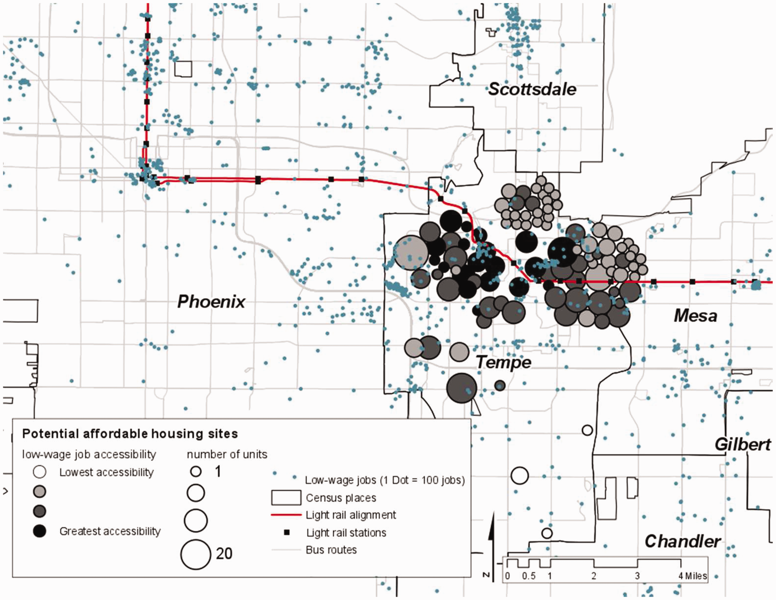

Construction cost estimates, based on US Census Bureau (2015) 2012–14 building construction cost data, were $236 thousand, $207 thousand, $149 thousand and $116 thousand per unit for single, two-unit, three-to-four unit, and five or more units per building, respectively. Estimation of the total construction budget refers to total construction cost in 2014, and we assume that 3% of all new housing construction (about $8 million) is used for constructing affordable housing units, ±5% (e.g. up to $8.4 million).⁷ The maximum number of housing units in each parcel is estimated using the parcel area divided by the minimum net site area (square feet) per dwelling. We assume that n, the number of low-income workers that each housing unit can serve, is two.

Figure 1 shows the public transit routes (sourced from Valley Metro's GTFS feed) and low-wage job locations (sourced from the LEHD dataset) in the Phoenix-Mesa-Glendale Metropolitan Area (MSA) and the accessibilities of all potential affordable housing sites in the City of Tempe. In South Phoenix (west of Tempe), there is very high density of transit routes combined with low-wage job clusters. Additionally, low-wage jobs are also clustered in North Tempe and South Scottsdale. High accessibility (darker shades) parcels are mostly located along transit routes with access to job clusters (e.g. the two parcels in the mid-west of Tempe and the parcels in the northwest of Tempe) and in areas with multiple routes that provide connectivity across job locations (e.g. the parcels clustered in northeast Tempe).

Results

Model size and computational performance

The model was built and solved using Xpress-IVE version 7.8 (FICO Xpress Optimization Suite). With 107 parcels i, the final model had 4498 constraints and 109 variables, of which 107 were integer X_i variables that can be relaxed and solved as continuous variables. The model was solved on a personal computer with 4 GB RAM and a 2.53 GHz CPU. The base case took 0.16 minutes to solve to global optimality.

Solutions

Under the assumption of a total construction budget of $8 million there are eight Pareto optimal solutions. Since the problem is a bi-objective integer programming problem, the Pareto front (tradeoff curve) of the problem is convex dominated and bounded by vectors (I, A) of solution 1 (0.00185, 6998890) and 8 (0.08081, 9937170) (Figure 2).

Figure 2.

Pareto-optimal tradeoff curve.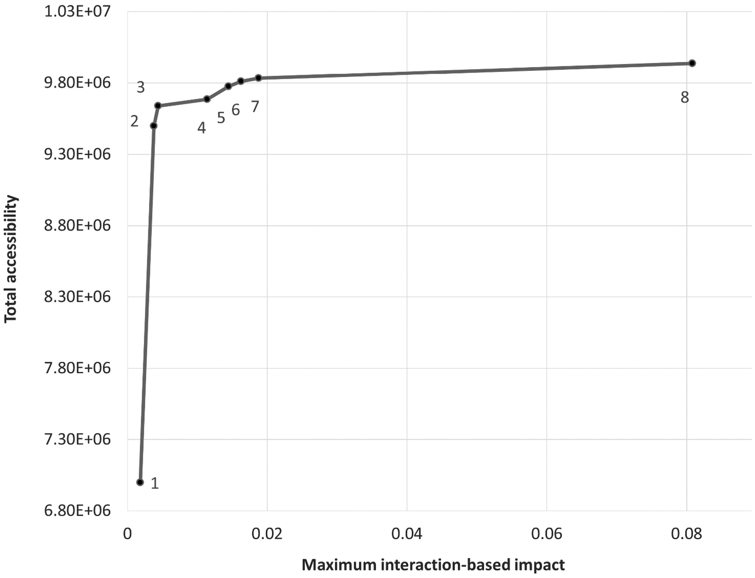

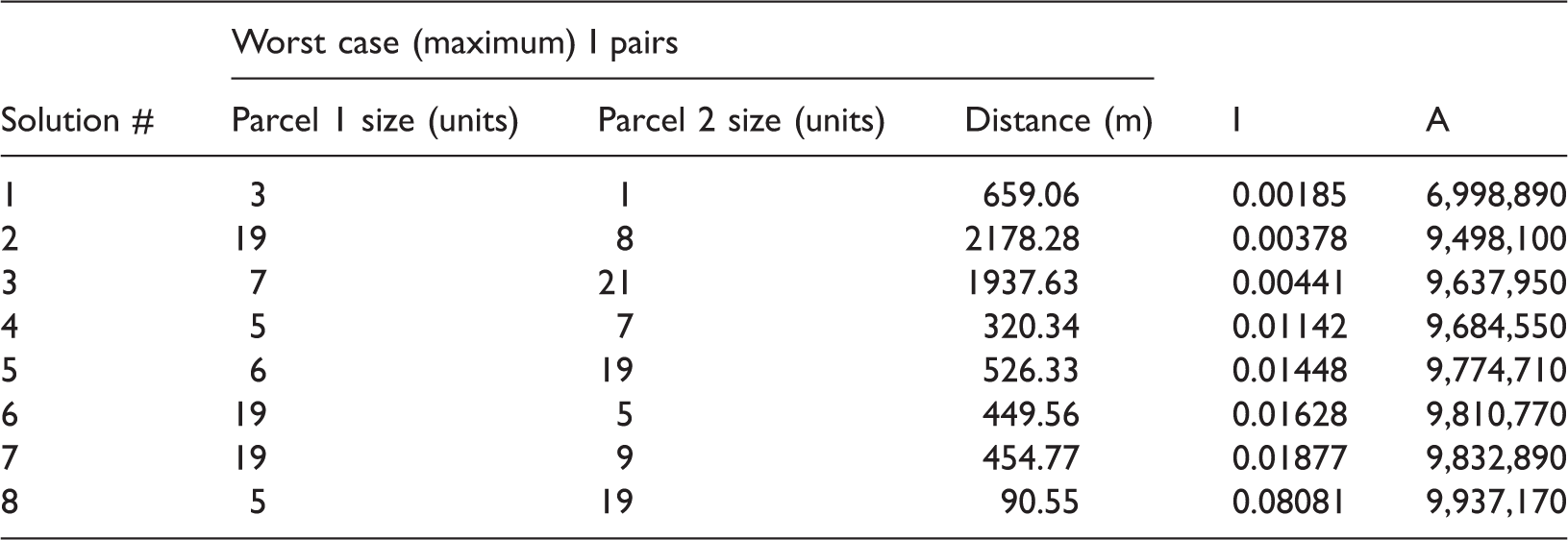
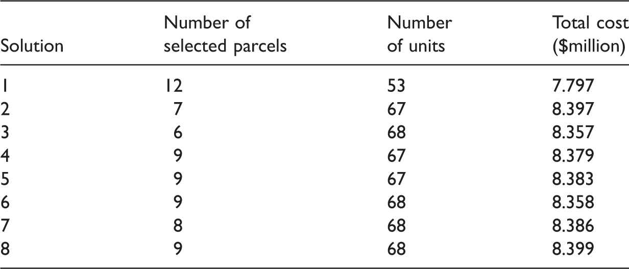
Figure 3 shows selected solutions to the problem. In solution #1, 12 parcels are selected to receive affordable housing. The distance between the worst case I pairs (parcels 6 and 30) is 659 m and the total units in the two locations is 4 (Table 1). In this case, the maximum impact on surrounding neighborhoods is the minimum among all the solutions, however, the total accessibility is also the minimum. Solution #2 has greatly improved the total accessibility (nearly 1.5 times of that of solution #1) by slightly increasing the value of the worst case impact. In this solution, there is a fairly long distance between the worst case I pairs (parcels 16 and 27), but the total number of units in the two locations (27) is very large, so the impact is the maximum among any two selected parcels. Similarly, solution #8 provides the highest total accessibility but the largest maximum impact value, while solution #7 greatly improves the worst case impact by sacrificing a small portion of total accessibility.

Figure 3.

Selected solutions to the problem, with parcel numbers labeled.

Table 1.

Worst case (maximum) I pairs of each solution.

Solution #	Worst case (maximum) I pairs			I	A
Solution #	Parcel 1 size (units)	Parcel 2 size (units)	Distance (m)	I	A
1	3	1	659.06	0.00185	6,998,890
2	19	8	2178.28	0.00378	9,498,100
3	7	21	1937.63	0.00441	9,637,950
4	5	7	320.34	0.01142	9,684,550
5	6	19	526.33	0.01448	9,774,710
6	19	5	449.56	0.01628	9,810,770
7	19	9	454.77	0.01877	9,832,890
8	5	19	90.55	0.08081	9,937,170

The objective of solving the multiobjective optimization problem is to support decision makers in finding the most preferred Pareto optimal solution according to their subjective preferences. Figure 2 and Table 1 demonstrate that there is not a lot of variation in total accessibilities and the worst case impacts from solution #2 to solution #7. The most preferred solution might be chosen from solutions #2 to #7 using different criteria other than the two objectives. For example, Table 2 shows some attributes that may affect location decisions outside of the two objective functions. Given the budget range, solution #3 provides the greatest number of units at the lowest construction cost.

Table 2.

Solution	Number of selected parcels	Number of units	Total cost ($million)
1	12	53	7.797
2	7	67	8.397
3	6	68	8.357
4	9	67	8.379
5	9	67	8.383
6	9	68	8.358
7	8	68	8.386
8	9	68	8.399

Sensitivity analysis

One concern we wish to address is whether there is a relationship between budget size and the solution pattern; if the general tradeoffs between burdens and benefits are not overly sensitive to budget size, we would expect similar behavior of the solution sets for different budgets. We modified the original $8 million budget to $4 million and $12 million and generated Pareto-optimal tradeoff curves for each (Figure 4). The smallest budget builds fewer housing units and affords less flexibility in distributing them across candidate sites, yielding a tradeoff curve with only three non-inferior solutions. As the budget increases, the curves move up (more total accessibility, due to more workers being housed) and to the right (higher maximum impact on neighborhoods, because there are more affordable housing complexes built on more parcels, forcing the worst-case pair closer together). Note that as a worst-case minimax objective, the dispersion of impact changes are much smaller in magnitude than those for the accessibility objective, which is structured as a sum of benefits over all parcels.

Figure 4.

Sensitivity analysis on construction budget.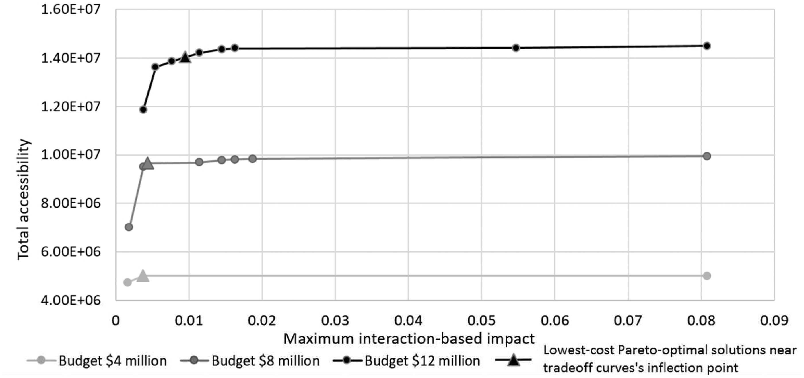

To compare the spatial arrangement of housing as the construction budget varies, we highlight a non-inferior solution on each curve near its inflection point (Figure 5). On the medium and large budget curves with multiple non-inferior solutions near the elbow, we selected the one with the lowest total construction cost (Table 3). Even in the high-budget scenario, the inflection-point solution is able to avoid choosing any sites from the two lowest accessibility categories.

Figure 5.

Solutions around the inflection points with the lowest cost, with parcel numbers labeled.

Table 3.

Attributes of the solutions around the inflection points with the low total cost.

Solution	Number of selected parcels	Number of units built	Total cost ($million)	Average A (per unit built)
High budget	12	100	12.509	140,511
Medium budget	6	68	8.357	141,735
Low budget	3	34	4.13	147,303

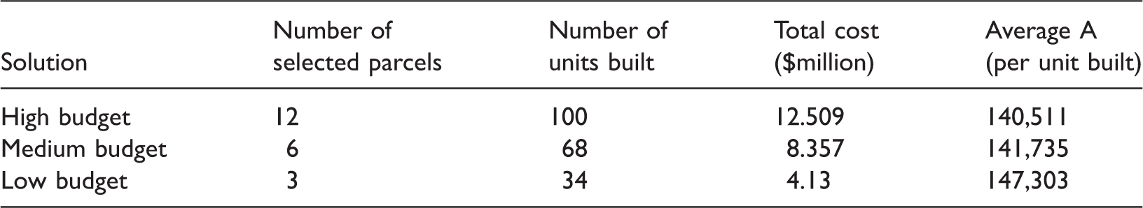
There is a surprising amount of consistency in the locations across these three solutions: all three locations chosen in the low-budget scenario are still optimal in the medium-budget scenario, and five of the six sites in the medium budget solution are still optimal in the 12-site high-budget solution. It appears that taking the size of locations into consideration in the dispersion objective creates stability in the solutions, allowing for greater robustness as a system of facilities scales up. Note also that the worst-case pair in each solution (contained in the red rectangle) remains in the solution for the next higher budget, but is no longer the worst case. Pair 16–27 is eclipsed by 60–62, which is eclipsed by 16–18 as the highest-impact pair.

Conclusion

The planning model in this paper was developed for spatial decision support to help affordable-housing providers design flexible strategies that maximize access to jobs while minimizing neighborhood impacts. The model builds on the substantial existing work by Johnson and others, but introduces several new approaches to the literature. First, it focuses explicitly on accessibility provided by public transportation to suitable jobs for low-wage workers. Second, it introduces a new minimax dispersion objective for spreading affordable housing across the study area based on spatial interaction principles of distance decay and additive facility sizes. The objectives of this multiobjective model are to maximize the total public transit accessibility of affordable housing units, and minimize the worst case where a large amount of affordable housing is located at two sites near each other. This worst case can be alleviated by reducing the number of units located in close proximity or increasing the distance by which they are separated. The data needed for this problem take into account size, cost, and zoning of vacant parcels, construction costs and total budget, travel time between parcels and jobs, number of jobs available, and bus and rail networks.

We applied the methodology to a case study of the City of Tempe, Arizona. All Pareto-optimal solutions were shown on the tradeoff curve, and selected Pareto-optimal solutions were analyzed and visualized. We also show several additional attributes that may aid the decision making process. A sensitivity analysis on the construction budget showed consistency in the shape of the tradeoff curves and stability in the locations as the system scales up. While built on the existing work in this area, these results are novel and result from significant modifications in the multi-objective models used compared to existing work. Even so, results are robust, sensible and informative, considering the tradeoffs between access and agglomeration of housing units.

For future work, a number of straightforward extensions would increase the realism and utility of the model. Existing public housing projects that are fixed in space (as opposed to housing vouchers) could be taken into account in dispersing new facilities from both existing and among new facilities. The provision of affordable housing may also be considered a benefit to employers, especially in tight job markets, and thus it might be desirable to maximize access by employers to potential low-wage employees living in subsidized housing. One could also model accessibility to additional kinds of services, like shopping, transportation infrastructure, childcare, good public schools, parks, cultural activities, health facilities, and counseling. Further analysis could be used to develop more realistic budget limits and unit costs to apply to a more realistic housing agency case study. Finally, results from models like this could be used within broader planning or advocacy campaigns to advance public-interest decision-making under complex trade-offs, like those found here in housing location choice (e.g. under a “community-based operations research model” Johnson, 2012; Midgley and Ochoa-Arias, 2004). This model could integrate into a broader process of regional housing advocacy or planning, where stakeholders would engage with the tradeoffs implied by the Pareto-optimal frontier, and use results for research to support housing policy and planning. Similarly, the emerging field of Geodesign, where collaborative stakeholder decision-making is augmented by visualization techniques combined with underlying performance models such as our two objective functions, could build on locational models like the one presented here (Foster, 2016; Steinitz, 2012).

Footnotes

Acknowledgements

The authors would like to thank the anonymous reviewers as well as the editor, Dr. Richard Harris, for their valuable feedback and guidance.

Declaration of conflicting interests

The author(s) declared no potential conflicts of interest with respect to the research, authorship, and/or publication of this article.

Funding

The author(s) received no financial support for the research, authorship, and/or publication of this article.

Notes

Qing Zhong is a PhD student in the School of Geography and Development at University of Arizona. Her research interests lie in spatial optimization, location analysis and modeling.

Alex Karner, PhD, is an Assistant Professor at The University of Texas at Austin’s Graduate Program in Community and Regional Planning. His work critically engages with the practice of transportation planning with the goal of achieving progress towards equity and sustainability. To this end, he develops innovative methods for analyzing the performance of integrated transportation‐land use systems in the areas of civil rights, environmental justice, public health, and climate change.

Michael Kuby is a professor in the School of Geographical Sciences and Urban Planning at Arizona State University, and Director of the Interdisciplinary Graduate Certificate in Transportation Systems. His research interests are in transportation, energy, network analysis and optimal facility location.

Aaron Golub is an Associate Professor in the Nohad A. Toulan School of Urban Studies and Planning at Portland State University. His teaching and research interests include the social impacts of transportation, planning for alternative transportation modes, and the history of transportation in the United States.

References

Bateman

Day

Georgiou

et al. (2006) The aggregation of environmental benefit values: Welfare measures, distance decay and total WTP. Ecological Economics 60(2): 450–460.

Bayram A, Solak S, Johnson M, et al. (2011) Stochastic dynamic models for foreclosed housing acquisition and redevelopment. In: Proceedings of the 2011 industrial engineering research conference, 2011, pp.1–8.

Benner

Karner

(2016) Low-wage jobs housing fit: Identifying locations of affordable housing shortages. Urban Geography 37(6): 883–903.

Blumenberg

Manville

(2004) Beyond the spatial mismatch: Welfare recipients and transportation policy. Journal of Planning Literature 19(2): 182–205.

Blumenberg

Ong

(2001) Cars, buses, and jobs: Welfare participants and employment access in Los Angeles. Transportation Research Record: Journal of the Transportation Research Board 1756: 22–31.

Chandrasekaran

Daughety

(1981) Location on tree networks: P-centre and n-dispersion problems. Mathematics of Operations Research 6(1): 50–57.

City of Tempe, Arizona (2015) Zoning and development code. Available at: www.tempe.gov/city-hall/community-development/planning/zoning-and-development-code.

Clifton

Lucas

(2004) Examining the empirical evidence of transport inequality in the US and UK. In: Lucas

(ed.) Running on Empty: Transport, Social Exclusion and Environmental Justice, Bristol, UK: The Policy PressAvailable at: http://trid.trb.org/view.aspx?id=790027.

Cohon

(1978) Multiobjective Programming and Planning, New York: Academic Press.

10.

Cutuli

Desjardins

Herbers

et al. (2013) Academic achievement trajectories of homeless and highly mobile students: Resilience in the context of chronic and acute risk. Child Development 84(3): 841–857.

11.

Daskin

(2011) Network and Discrete Location: Models, Algorithms, and Applications, New York: John Wiley & Sons.

12.

Erkut

Neuman

(1989) Analytical models for locating undesirable facilities. European Journal of Operational Research 40(3): 275–291.

13.

ETC Institute (2011) 2010–2011 Transit On-Board Survey Final Report, Valley Metro Rapid Transit DistrictAvailable at: http://www.valleymetro.org/images/uploads/projects/2010-2011_Transit_On-Board_Survey_Final_Report.pdf.

14.

Farber

Morang

Widener

(2014) Temporal variability in transit-based accessibility to supermarkets. Applied Geography 53: 149–159.

15.

Forgionne

(1991) HANS: A decision support system for military housing managers. Interfaces 21(6): 37–51.

16.

Forgionne

(1997) HADTS: A decision technology system to support Army housing management. European Journal of Operational Research 97(2): 363–379.

17.

Forgionne

Frager

(1998) The US Army relies on decision support systems in allocating housing resources. Interfaces 28(2): 72–79.

18.

Foster

(2016) Geodesign parsed: Placing it within the rubric of recognized design theories. Landscape and Urban Planning 156: 92–100.

19.

Fransen

Neutens

Farber

et al. (2015) Identifying public transport gaps using time-dependent accessibility levels. Journal of Transport Geography 48: 176–187.

20.

Garrett

Taylor

(1999) Reconsidering social equity in public transit. Berkeley Planning Journal 13: 6–27.

21.

Geurs

van Wee

(2004) Accessibility evaluation of land-use and transport strategies: Review and research directions. Journal of Transport Geography 12(2): 127–140.

22.

Gobillon

Selod

Zenou

(2007) The mechanisms of spatial mismatch. Urban Studies 44(12): 2401–2427.

23.

Golub

Martens

(2014) Using principles of justice to assess the modal equity of regional transportation plans. Journal of Transport Geography 41: 10–20.

24.

Golub

Robinson

Nee

(2013) Making accessibility analyses accessible: A tool to facilitate the public review of the effects of regional transportation plans on accessibility. Journal of Transport and Land Use 6(3): 17–28.

25.

Grengs

(2010) Job accessibility and the modal mismatch in Detroit. Journal of Transport Geography 18(1): 42–54.

26.

Handy

Niemeier

(1997) Measuring accessibility: An exploration of issues and alternatives. Environment and Planning A 29(7): 1175–1194.

27.

Hanley

Schläpfer

Spurgeon

(2003) Aggregating the benefits of environmental improvements: Distance-decay functions for use and non-use values. Journal of Environmental Management 68(3): 297–304.

28.

HousingPolicy.org (2016) What is affordable housing? Available at: www.housingpolicy.org/getting_started/what.html#What+is+%22affordable+housing%22%3F.

29.

Ihlanfeldt

Sjoquist

(1998) The spatial mismatch hypothesis: A review of recent studies and their implications for welfare reform. Housing Policy Debate 9(4): 849–892.

30.

Immergluck

(1998) Job proximity and the urban employment problem: Do suitable nearby jobs improve neighbourhood employment rates?. Urban Studies 35(1): 7–23.

31.

Johnson

(2003) Single-period location models for subsidized housing: Tenant-based subsidies. Annals of Operations Research 123(1–4): 105–124.

32.

Johnson

(2006) Single-period location models for subsidized housing: Project-based subsidies. Socio-Economic Planning Sciences 40(4): 249–274.

33.

Johnson

(2007) Planning models for the provision of affordable housing. Environment and Planning B: Planning and Design 34(3): 501–523.

34.

Johnson

(2012) Community-based operations research: introduction, theory, and applications. In: Community-Based Operations Research, New York: Springer.

35.

Johnson

Hollander

Hallulli

(2014) Maintain, demolish, re-purpose: Policy design for vacant land management using decision models. Cities 40: 151–162.

36.

Johnson

Hurter

(1998) An optimization model for location of subsidized housing in metropolitan areas. Location Science 6(1): 257–279.

37.

Johnson

Hurter

(2000) Decision support for a housing mobility program using a multiobjective optimization model. Management Science 46(12): 1569–1584.

38.

Johnson

Ladd

Ludwig

(2002) The benefits and costs of residential mobility programmes for the poor. Housing Studies 17(1): 125–138.

39.

Johnson

Turcotte

Sullivan

(2010) What foreclosed homes should a municipality purchase to stabilize vulnerable neighborhoods?. Networks and Spatial Economics 10(3): 363–388.

40.

Kaplan

(1986) Tenant assignment models. Operations Research 34(6): 832–843.

41.

Kaplan

Berman

(1988) OR hits the heights: Relocation planning at the orient heights housing project. Interfaces 18(6): 14–22.

42.

Karner A (2017) Assessing public transit service equity using route-level accessibility measures and public data. Working paper.

43.

Karsu

Morton

(2015) Inequity averse optimization in operational research. European Journal of Operational Research 245(2): 343–359.

44.

Kotz

(2011) The Spatial Concentration of Subsidized Housing, Doctoral Dissertation, University of DelawareAvailable at: http://www.prrac.org/pdf/Kotz_Dissertation_12-5-11.pdf.

45.

Kuby

(1987) Programming models for facility dispersion: The p-Dispersion and Maxisum Dispersion Problems. Geographical Analysis 19(4): 315–329.

46.

Lens

(2014) Employment accessibility among housing subsidy recipients. Housing Policy Debate 24(4): 671–691.

47.

Lubell

Crain

Cohen

(2007) Framing the issues—The positive impacts of affordable housing on health. Center for Housing Policy 34. .

48.

Midgley

Ochoa-Arias

(2004) Community Operational Research – OR and Systems Thinking for Community Development, US: Springer.

49.

Nguyen

(2005) Does affordable housing detrimentally affect property values? A review of the literature. CPL Bibliography 20(1): 15–26.

50.

Ong

Blumenberg

(1998) Job access, commute and travel burden among welfare recipients. Urban Studies 35(1): 77–93.

51.

Owen

Levinson

(2014) Access Across America: Transit 2014, Minneapolis, MN: Accessibility Observatory, University of Minnesota.

52.

Paez

Mercado

Farber

et al. (2010) Accessibility to health care facilities in Montreal Island: An application of relative accessibility indicators from the perspective of senior and non-senior residents. International Journal of Health Geographics 9(1): 52.

53.

Pucher

Renne

(2003) Socioeconomics of urban travel: Evidence from the 2001 NHTS. Transportation Quarterly 57(3): 49–77.

54.

Public Policy Institute of California (PPIC) (2004) How Much Do Low-Income Californians Pay for Transportation? Research Brief 91. Available at: http://www.ppic.org/content/pubs/rb/RB_704LRRB.pdf.

55.

Rafferty

Shinn

Weitzman

(2004) Academic achievement among formerly homeless adolescents and their continuously housed peers. Journal of School Psychology 42(3): 179–199.

56.

Ratick

White

(1988) A risk-sharing model for locating noxious facilities. Environment and Planning B: Planning and Design 15(2): 165–179.

57.

Rosenbloom

(1998) Transit Markets of the Future: The Challenge of Change, TCRP Report 28. Washington DC: Transportation Research Board.

58.

Schwartz

(2010) Housing Policy in the United States, New York: Routledge.

59.

Shen

(1998) Location characteristics of inner-city neighborhoods and employment accessibility of low-wage workers. Environment and Planning B: Planning and Design 25(3): 345–365.

60.

Shen

(2001) A spatial analysis of job openings and access in a U.S. metropolitan area. Journal of the American Planning Association 67(1): 53–68.

61.

Steinitz

(2012) Framework for Geodesign: Changing Geography through Design, Redlands: ESRI Press.

62.

Tamir

(2006) Locating two obnoxious facilities using the weighted maximin criterion. Operations Research Letters 34(1): 97–105.

63.

Taylor

Morris

(2015) Public transportation objectives and rider demographics: Are transit's priorities poor public policy?. Transportation 42(2): 347–367.

64.

Taylor

Ong

(1995) Spatial mismatch or automobile mismatch? An examination of race, residence and commuting in US metropolitan areas. Urban Studies 32(9): 1453–1473.

65.

Tighe

(2010) Public opinion and affordable housing: A review of the literature. Journal of Planning Literature 25(1): 3–17.

66.

US Census Bureau (2015) Building permits data, 2012–2014. Available at: http://censtats.census.gov/cgi-bin/bldgprmt/bldgdisp.pl.

67.

US Department of Housing Urban Development (2015) Affordable housing. Available at: https://portal.hud.gov/hudportal/HUD?src=/program_offices/comm_planning/affordablehousing.

68.

Welch

(2013) Equity in transport: The distribution of transit access and connectivity among affordable housing units. Transport Policy 30: 283–293.

69.

Zhang

Liu

Chen

et al. (2013) Using GIS and KDE analysis spatial distribution on public housing households: A case study. In: 8th international conference on computer science & education (ICCSE), 2013, New York: IEEE, pp. 925–930. .

70.

Zhang

Liu

et al. (2009) Application of GIS and spatial decision support system for affordable housing. In: 4th international conference on computer science & education, 2009. ICCSE'09, New York: IEEE, pp. 1110–1115. .