
Abstract
Robust calibration and validation of applied urban models are prerequisites for their successful, policy-cogent use. This is particularly important today when expert assessment is questioned and closely scrutinized. This paper proposes a new model calibration-validation strategy based on a spatial equilibrium model that incorporates multiple time horizons, such that the predictive capabilities of the model can be empirically tested. The model is implemented for the Greater Beijing city region and the model validation strategy is demonstrated over the Census years 2000 to 2010. Through forward/backward forecasting, the model validation helps to verify the stability of the model parameters as well as the predictive capabilities of the recursive equilibrium framework. The proposed modelling strategy sets a new standard for verifying and validating recursive equilibrium models. We also consider the wider implications of the approach.
Keywords
Introduction
Urban land use and transport interaction (LUTI) models have been the mainstay of practical policy analyses over the past decades. Originating from early applications of spatial interaction (Batty and Mackie, 1972; Echenique et al, 1969; Lowry, 1964), the model structure and equations have undergone remarkable transformations through, e.g. the incorporation of general equilibrium theory in urban and regional economics (Anas and Liu, 2007; Bröcker, 1998) on one end of the spectrum to the adoption of disaggregate, microscopic and agent-based spatial simulation on the other (Heppenstall et al., 2011). In contrast, research into the predictive capabilities of these models has progressed less quickly. Model validation in its strict sense (i.e. comparison between model outputs and observed data that have not been used in model calibration) is just as rarely practised today as decades ago. In the current climate where expert opinion is questioned, it is vital to develop model validation strategies that are robust and comprehensible. This is particularly challenging in fast growing cities in developing countries where the pressures for development are high while data provision for modelling is poor.
A sound understanding of the predictive capabilities of a LUTI model is a prerequisite for its use in practical projects regarding investment or regulation in cities. Systematic reviews of urban applied models, such as Wegener (1994, 2004), have always given due prominence to model calibration and validation. Since such reviews already exist, we do not intend to carry out a full literature survey. Instead, we focus on specific issues regarding validating the model over time, which is an under-researched field.
On cross-sectional model validation, Wegener (1994, 2004) points out that if model calibration is limited to only one temporal cross-section, then it provides little more than an illusion of precision. This is because model fitting techniques today have made it easier than ever before to reproduce any observed temporal cross-section. The pursuit for ever better goodness-of-fit at that cross-section alone does not necessarily indicate the actual predictive capabilities of a LUTI model. He further suggests that a model’s performance should be validated by comparing the model results with observed data over a relatively long period.
As an indication of what policy analysts may think, Volterra et al. (2007) provide an extensive review of the urban land-use and transport modelling practice in London, UK. They conclude from the London experience that model validation is particularly difficult given both data and time constraints, albeit the task is ‘completely necessary’ in a policy context. They also propose that a feasible approach to validate urban models is to create retrospective (historical) forecasts and compare them to observed histories.
Although there is consensus among the leading modellers on what should be done on model validation, there are theoretical as well as practical barriers in turning the consensus aspiration into practice in most LUTI applications. Finding suitable time series data is a common, practical challenge. However, as a number of LUTI models have been developed over the past years, the data and model predictions produced by those projects would represent a valuable resource for both supporting long time series of land use and transport data, as well as carrying out retrospective analysis of the models’ predictive performance. For cities that do not yet have their own LUTI models, it would be beneficial to design new modelling projects so that a time series of land use and transport data and predictions are gradually accumulated.
For LUTI models that are based on static general equilibrium, there is also an issue of how to compare model results that are not time specific with observations that are collected for specific temporal cross-sections. Similarly, for microscopic, agent-based non-equilibrium dynamic models, the issue is how to translate the probabilistic predictions of, e.g. the transitional states of building use into an evolutionary perspective of how buildings, infrastructure and activities change over time in a real context.
A rare and inspiring example of validating large-scale urban land-use and transport models is reported in Miller et al. (2012). They present the historical validation of their ILUTE model, an agent-based microsimulation model, for the greater Toronto area over a time span of 20 years (1986–2006). Model forecasts on demographics and the housing market are compared with historical data and a decent level of goodness of fit is achieved over multiple time horizons. This work shows that the technical difficulties of model validation are not insurmountable, and the field will greatly benefit from a closer examination of the predictive capabilities of models over time.
Our paper aims to fill a gap in the literature by proposing a new model calibration-validation strategy based on a spatial equilibrium model that incorporates multiple time horizons. The proposed strategy makes use of observed land use, buildings, transport and urban activity data across multiple time horizons such that the predictive capabilities of the model can be empirically tested.
The paper is organized as follows. The next section introduces the core structure of the model application for Greater Beijing. ‘Model calibration’ section discusses data and model calibration, ‘Model validation’ section presents the model validation strategy and its application to Greater Beijing and ‘Conclusions’ section considers wider implications of the findings.
Model description
The distinct feature of the Recursive-dynamic Spatial Equilibrium (RSE) model is the link between Spatial Equilibrium (SE) and Recursive Dynamic (RD) models, which enables the simulation of urban change processes that vary over time scales (Simmonds et al., 2013; Wegener et al., 1986). Some urban change processes (e.g. workplace relocation and transport choices) adapt quickly to circumstance changes and thus are amenable to equilibrium modelling, while others are more inertia-prone and may take many years or even decades to adjust (e.g. building stock development and transport supply). In this section, we focus on new advancements in the RSE model since its early prototype in Jin et al. (2013), and introduce how the RSE model is calibrated and validated over multiple time horizons. More details about the model including the equations and equilibrium conditions are provided in the online Supplementary Material.
The theoretical RSE model is first proposed in Jin et al. (2013). In that paper, the recursive-dynamic feature of the model is demonstrated on a hypothetical peninsular city, where no empirical data are used for model calibration or validation. The RSE Greater Beijing model presented here differs from Jin et al. (2013) by incorporating the following advancements. First, we complete the general equilibrium structure of the SE model by incorporating a new equilibrium condition for the labour market. In Jin et al. (2013), the derived workplace wage is vaguely defined without equilibrating the zonal labour demand and supply. In this paper, the SE framework entails simultaneous equilibrium in production, floorspace and labour markets, subject to supply constraints and policy interventions. Second, we substitute the multinomial-logit discrete choice model with a nested-logit model for simulating the employment-residence paired location choices; the nested-logit model is theoretically more consistent, because it captures the correlations that exist among location alternatives. Third, generic methods for establishing and calibrating the RD models for floorspace development are developed, which is supported by economic theory and amenable to statistical analysis; the proposed models account for not only the physical durability of buildings but also the regional heterogeneity and one-off policy interventions. Fourth, the recursive-dynamics is extended from modelling building floorspace growth to residence relocation of non-employed households.
To demonstrate how the RSE model is calibrated and validated over multiple time horizons before being used for model forecasting, Figure 1 illustrates the information flows in the RSE model. Three time horizons are presented in the figure from time t to t + 2, where time t and t + 1 are historical in the sense that known data are available and time t + 2 is the future year. The SE model calibration at base year t follows the standard procedure as per conventional static equilibrium models. The novelty of the RSE model is that for the model calibrated at time t, its predictive capabilities can be empirically tested through forward forecasting from time t to t + 1, by comparing the model outputs with the known data set for time t + 1. To build up a serial track record, the forecasted results for time t + 2 can also be validated when the observed data set for time t + 2 becomes available.
Main information flows within and between recursive spatial equilibria.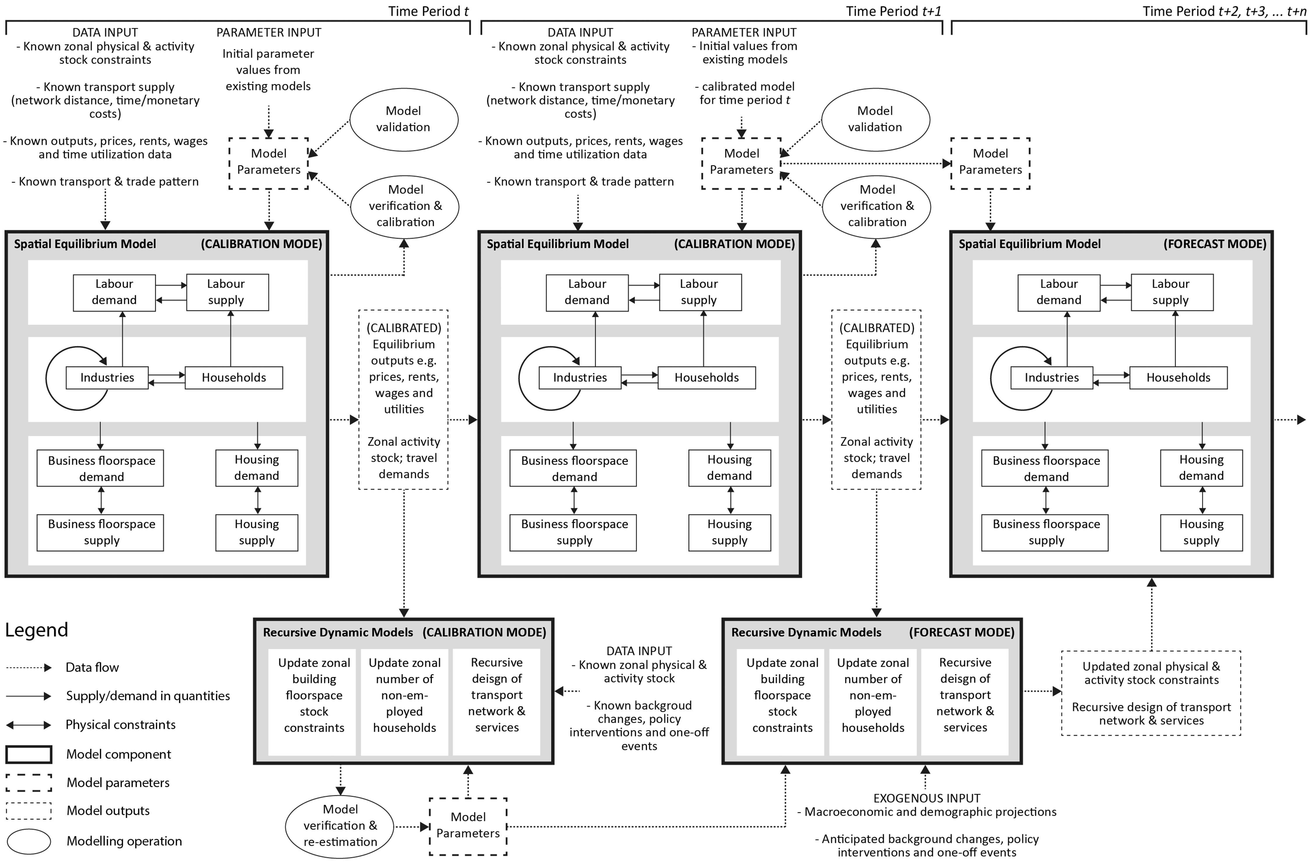
In practice, it is rarely feasible to trace back more than one historical period for data problems and modeller resources. An alternative way to validate the SE model for time t + 1 is to forecast backwards to time t, using the zonal stock constraints of time t as inputs. This process is counterfactual in nature, but it serves a dual purpose: (1) it helps modellers to crosscheck the data sets over two consecutive cross sections; and (2) as the forward and backward forecasts essentially involve two sets of model parameters, by comparing the performance of the two models, modellers can better understand the background changes in reality as well as the role of key parameters in model predictions. The proposed modelling method sets a new standard for verifying and validating recursive equilibrium models.
Once the SE model is calibrated at base year t, the RD models are then calibrated using model outputs from the SE model for time t, observed changes in zonal stock and the knowledge on policy interventions (including one-off events) from t to t + 1. The SE and RD model calibration may have to be repeated many times in a calibration-validation loop until a satisfactory goodness of fit has been achieved. After the model validation, the RSE model will operate in forecast mode with model parameters retained for further years.
Model application for Greater Beijing
The RSE Greater Beijing Model is the first empirical application of the RSE model since Jin et al. (2013). The model is designed for examining medium- to long-term impacts of major urban land-use and transport development options. Its potential use in practical policy analysis is reported in Jin et al. (2017). The model covers the administrative area of Beijing, Tianjin and Hebei in China (locally known as the ‘Jing-Jin-Ji’ city region), which has a total population of approximately 110 million in 2014 across a geographical area of over 216 thousand km2. The Greater Beijing city region is represented by a total of 209 model zones (Figure 2). We define the 130 zones of Beijing Municipality as core zones of study and the 79 zones of Tianjin and Hebei as peripheral zones. For the core zones in Beijing, the zoning is based on the administrative boundaries of Jiedao, which is the smallest areal administrative unit in China and the finest geographic level for Census statistics.
Zoning map of Greater Beijing (employment density in 2010).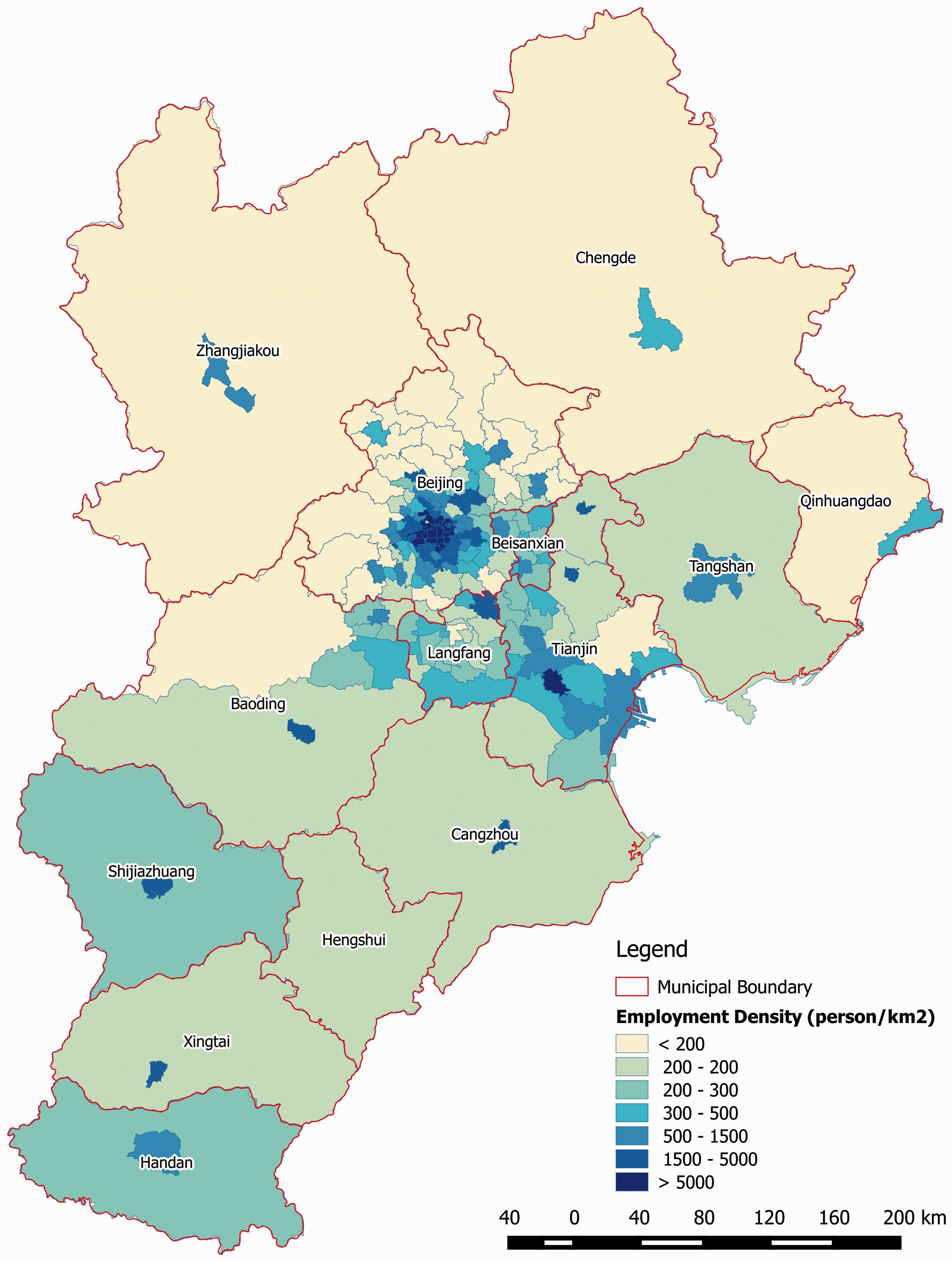
Segmentations in the RSE Greater Beijing model.
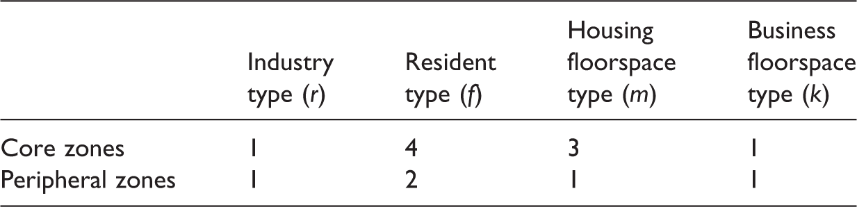
RSE: Recursive-dynamic Spatial Equilibrium.
In the RSE Greater Beijing model, residents as well as jobs are mobile across the city region subject to market inertia and specific boundary settings. The housing and business floorspace development, transport infrastructure supply and the relocation of non-employment households are treated as stock constraints. Such constraints are unchangeable in static equilibrium, implying the inertia-prone nature of the respective market, but are subsequently updated through the RD models in a recursive manner.
Model calibration
Before embarking on the discussion on model validation, we first introduce the calibration of the RSE Greater Beijing model and the associated data inputs. Specifically we start from an overview of the growth in Greater Beijing from 2000 to 2010 using aggregate statistics. Then the items for calibrating the SE and RD models are presented in turn.
Data
To prepare the data sets for the RSE Greater Beijing model, we combine various data sources, including the official statistics, censuses, surveys as well as online open data sources to complete the data set. Data that are unavailable are either estimated from supporting sources or assumptions are made. In such cases, we crosscheck the estimations with aggregate statistics and modellers’ local knowledge.
Demographics and building stock changes in Greater Beijing (2000–2010).
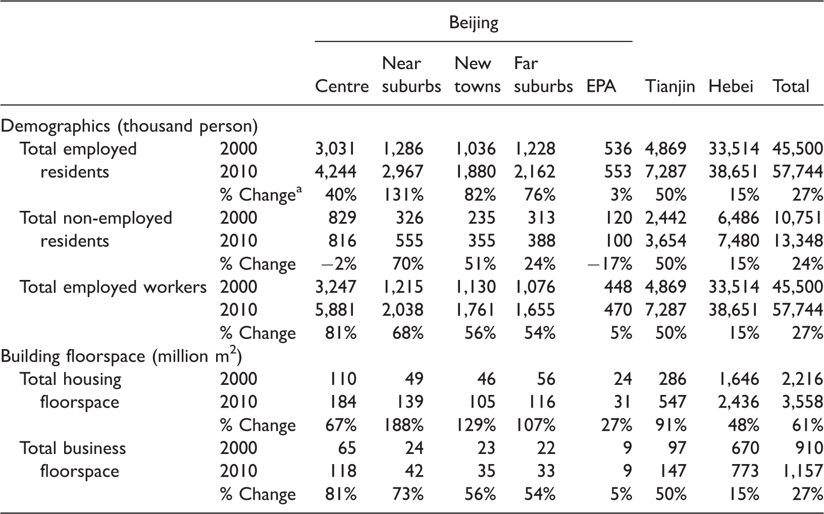
EPA: ecological protection areas.
% Change: based on the 2000 value.
Calibrating the SE model
Parameters and data inputs for Spatial Equilibrium model calibration.
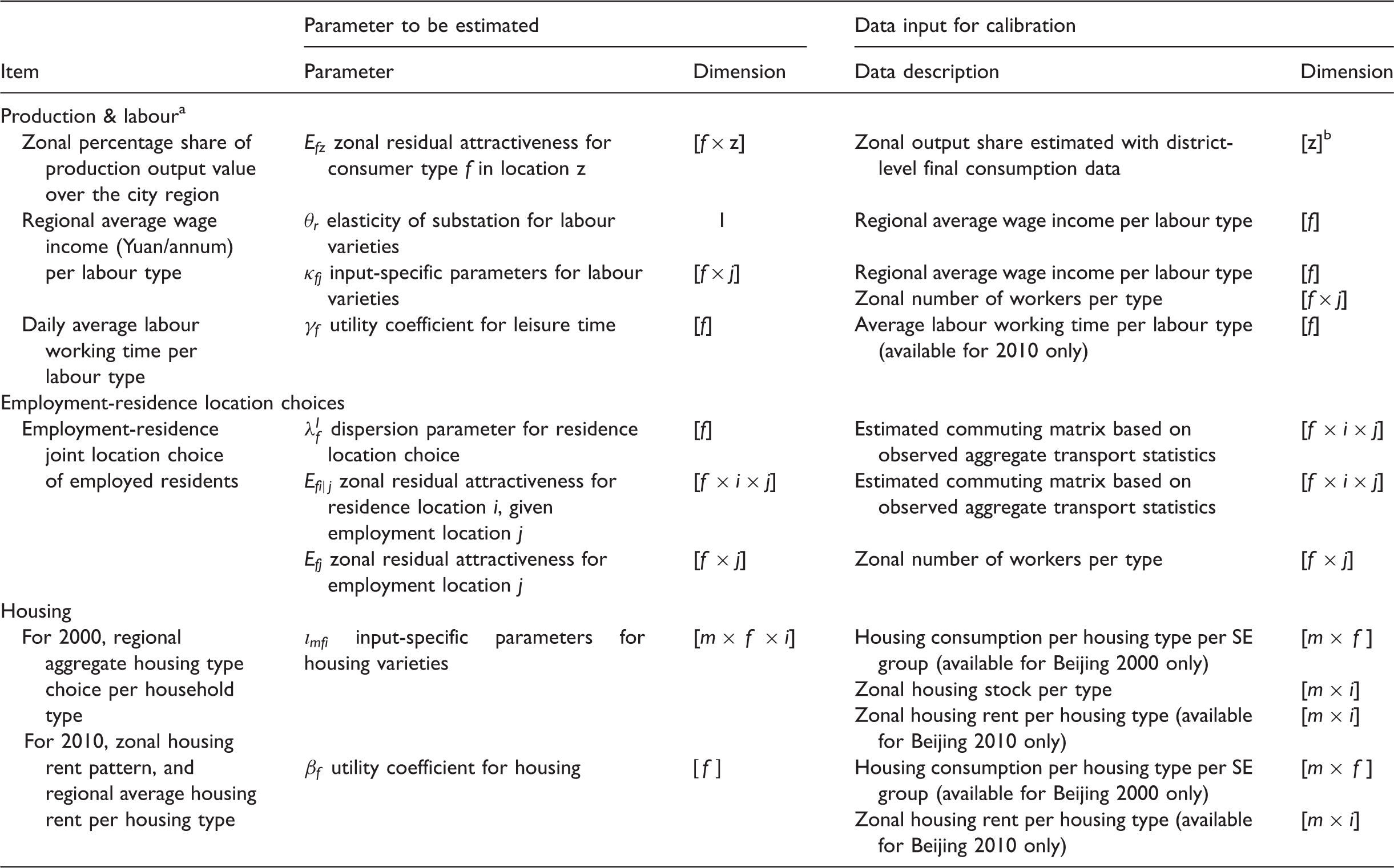
The intermediate demand for production is omitted from the theoretical model due to lack of data.
The estimated zonal final consumption data do not include the breakdown of different socio-economic groups. Therefore, we assume uniform parameters for all socio-economic groups.
Note that for production and labour, we calibrate the zonal production output by the percentage share over the region, rather than using the absolute output value. This is because the actual production output or sales data are not currently available in Greater Beijing and we use the processed final consumption data as a proxy. Second, as no zonal wage data are available in Greater Beijing, we make use of the regional average wage for each labour type to calibrate wages at the aggregate level. The zonal wage pattern is manually examined with modeller’s local knowledge. Third, in the RSE model, employed consumers can trade off between working and leisure in terms of time utilization under budget and time constraints. The value of unit leisure time is measured by the opportunity cost, namely hourly wage. The trade-off behaviour is calibrated with the Time Utilization Survey (National Bureau of Statistics (NBS), 2008) data in Beijing. Fourth, for calibrating the housing market, the zonal housing rent data are only available for the year 2010, and thus the housing rent calibration applies to the 2010-year model only. Nonetheless, for the 2000-year model, an alternative data set (i.e. housing consumption data per housing type per household type) is available to calibrate the housing type choices at the aggregate level. In addition, we do not calibrate the constant elasticity of substitution
Calibrating the RD models
Parameters and data inputs for Recursive Dynamic model calibration.
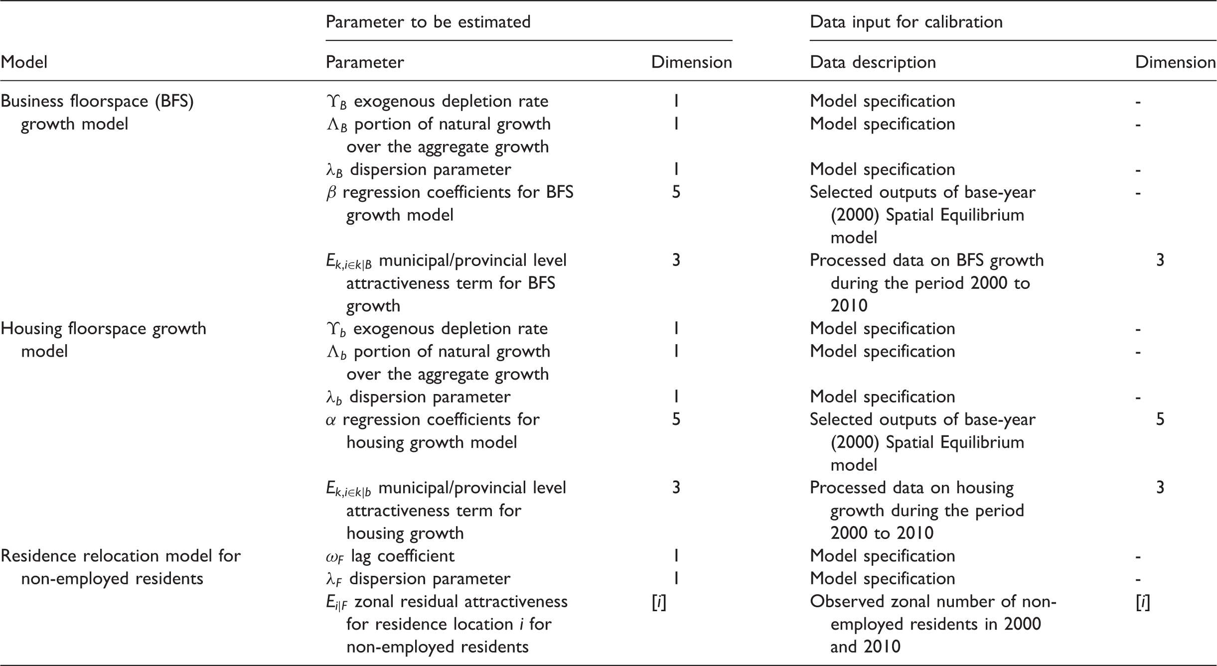
The proposed stock-updating mechanism refers to not only the endogenous market variables from the SE model, but also the durability of development and one-off policy interventions. We account for the spatial heterogeneity in floorspace growth by incorporating a set of residual terms for municipal/provincial locations (Ek). This new model specification facilitates the model application to large city regions, where significant heterogeneity across the cluster of cities often exists for historical, geographical and institutional reasons. This new model parameter is identified through the proposed calibration-validation loop, where predictive discrepancies between the modelled and the observed are investigated to improve the model performance. In the next section, we present the model validation through forward and backward forecasting.
Model validation
The calibrated RSE model needs to be validated before forecasting. By validation, we first operate the calibrated SE for 2000 to predict forwards for 2010, and compare the model predictions with the known data set. The forward forecast validates the predictive capabilities of the calibrated SE model for 2000. We then use the calibrated SE model for 2010 to predict backwards for 2000. This hypothetical backward forecast serves as an alternative to validate the SE model for 2010, when the forward forecast for 2020 is not yet available.
Validating the RD models ideally requires data for at least one more transitional period other than the 2000–2010 period, which is currently not available. Alternatively, we use the in-sample validation method, i.e. the model is estimated with a partial data set, while the remainder is used to validate the calibrated model. In the next section, we discuss the validation of the SE and RD models in turn.
SE model: Forward forecast from 2000 to 2010
Data inputs for the forward forecast (from 2000 to 2010).
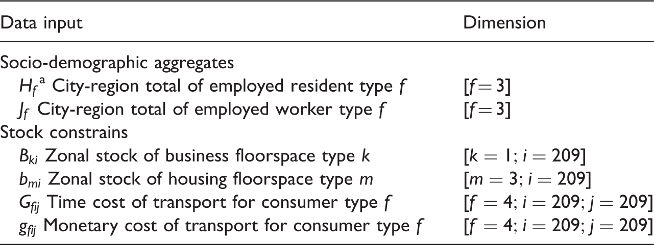
For the non-employed residents, we take the zonal totals as inputs because the residence relocation of the non-employed residents is modelled with RD models rather than the SE model. Thus we do not consider it for validation.
Given the exogenous inputs, the calibrated SE model for 2000 predicts the zonal prices, rents and quantities for the year 2010. In this paper, the model validation is focused on the spatial distribution of employed residents (ER) and workers (EW). Specifically we compare the modelled zonal number of ER and EW with the known data set for 2010 through scatter plots (Figure 3). In the scatter plot, the thick red line is the y = x reference line representing a perfect fit.
Validation through the forward forecast – EW/ER observed vs. modelled.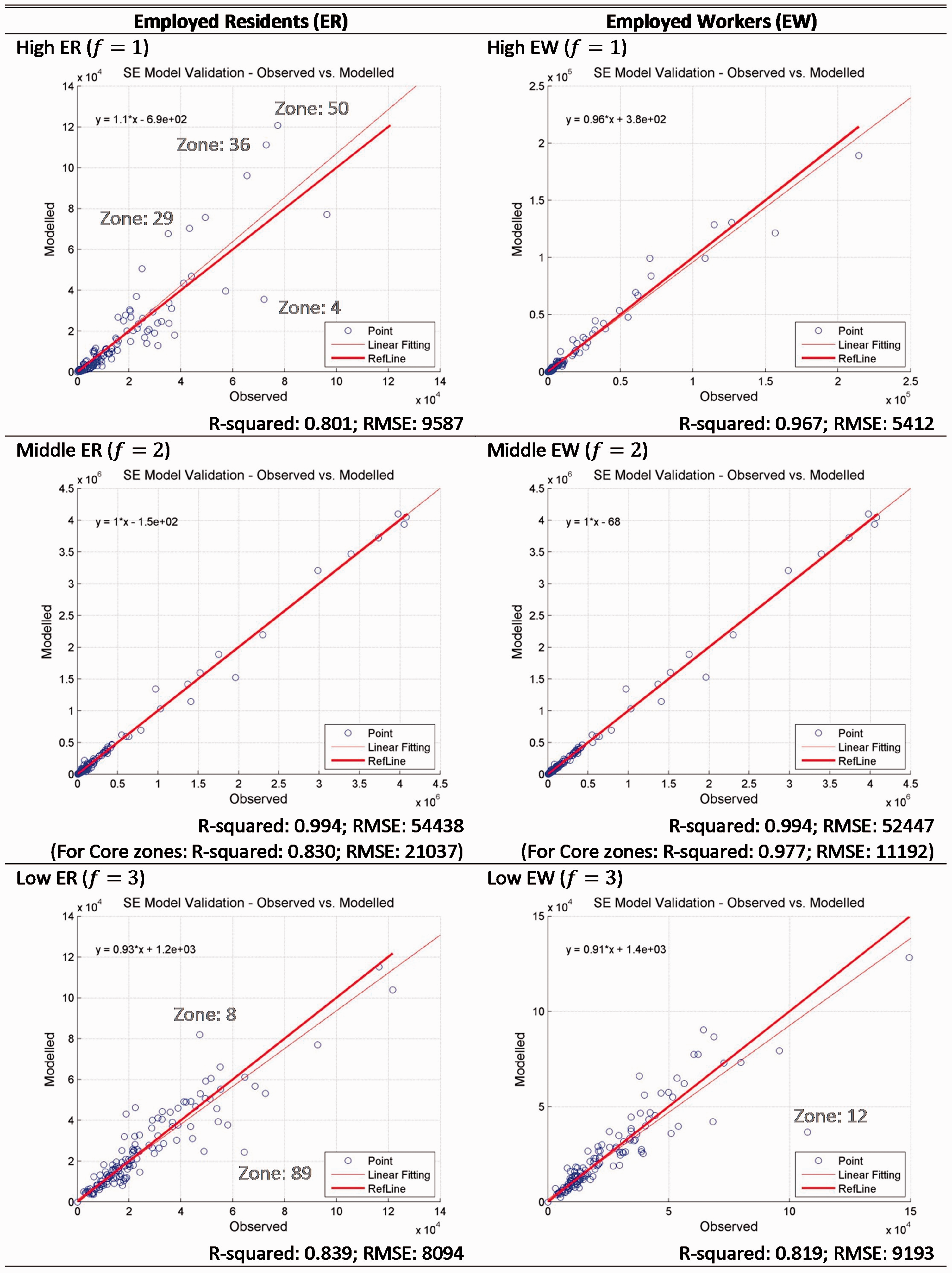
Notes on outliers – forward forecast.
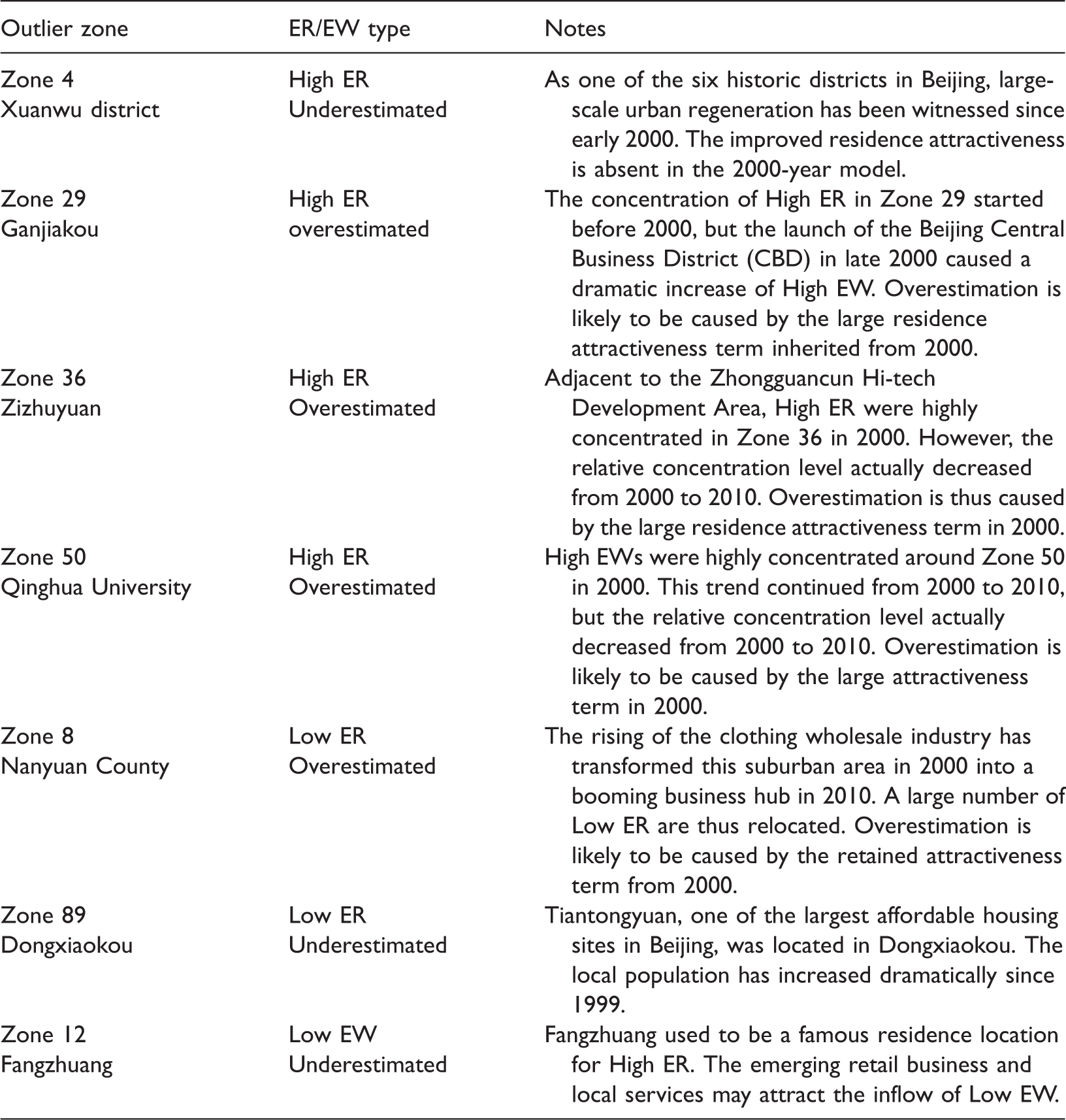
ER: employed residents; EW: employed workers.
Two major sources of discrepancy are identified: (1) the use of constant parameters, particularly the residual terms reflecting locational idiosyncratic attractiveness; and (2) exogenous policy interventions and other one-off events. Apart from these outliers, the model calibrated to the census year 2000 is shown to be capable of generating predictions for the year 2010 that are consistent with the observed patterns. This implies that the SE framework captures the fundamental market mechanisms that are relatively persistent over time. In the next section we conduct the backward-forecast validation from year 2010 to 2000.
SE model: Backward forecast from 2010 to 2000
In the backward forecast, we use the SE model calibrated for 2010 to predict the market conditions of 2000. The data inputs required are the same as listed in Table 5, but are for the year 2000 instead of 2010. We compare the predicted zonal number of ER and EW for 2000 with the known data set through scatter plots (Figure 4).
Validation through the backward forecast – EW/ER observed vs. modelled.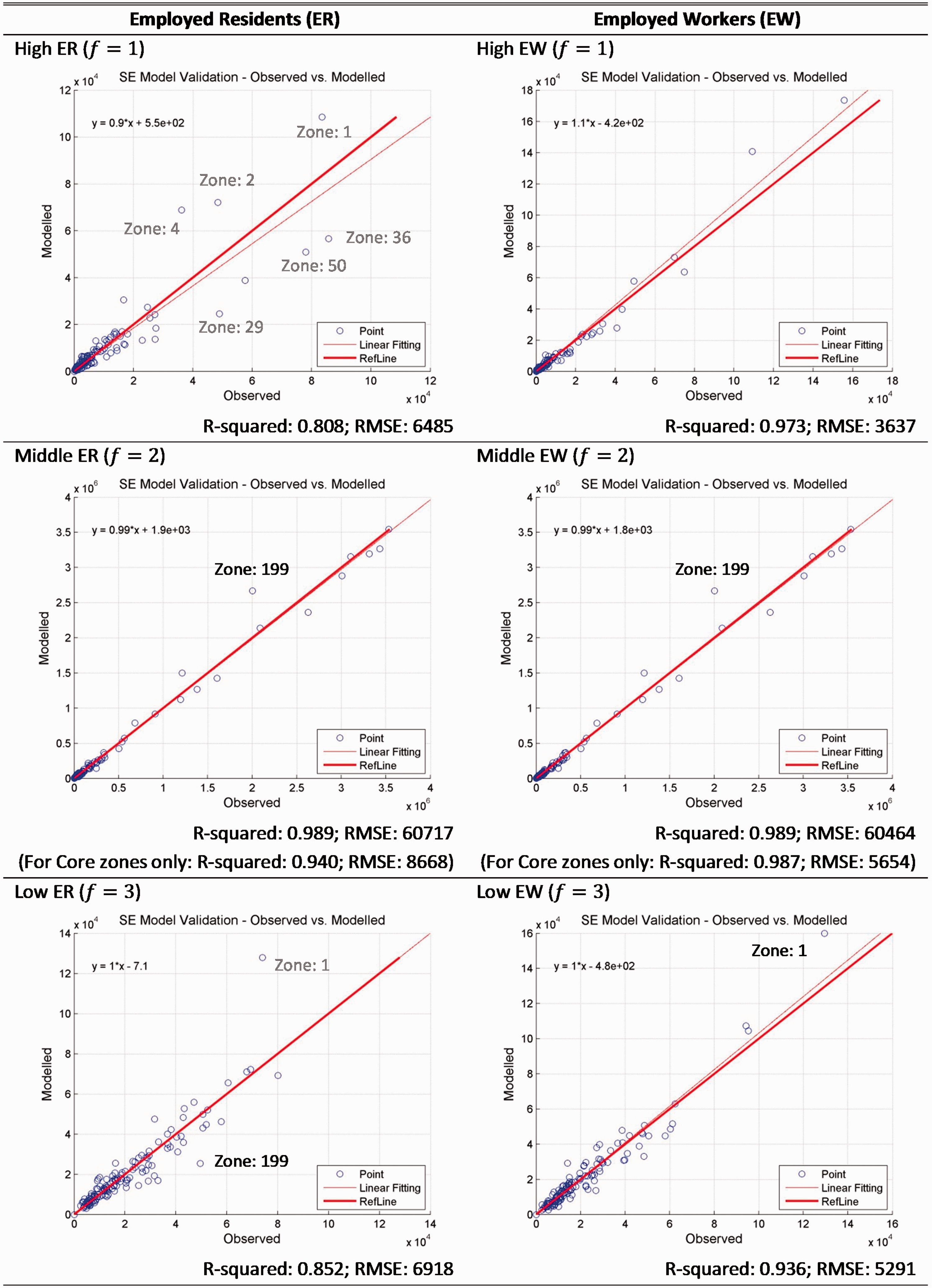
Notes on outliers – forward forecast.
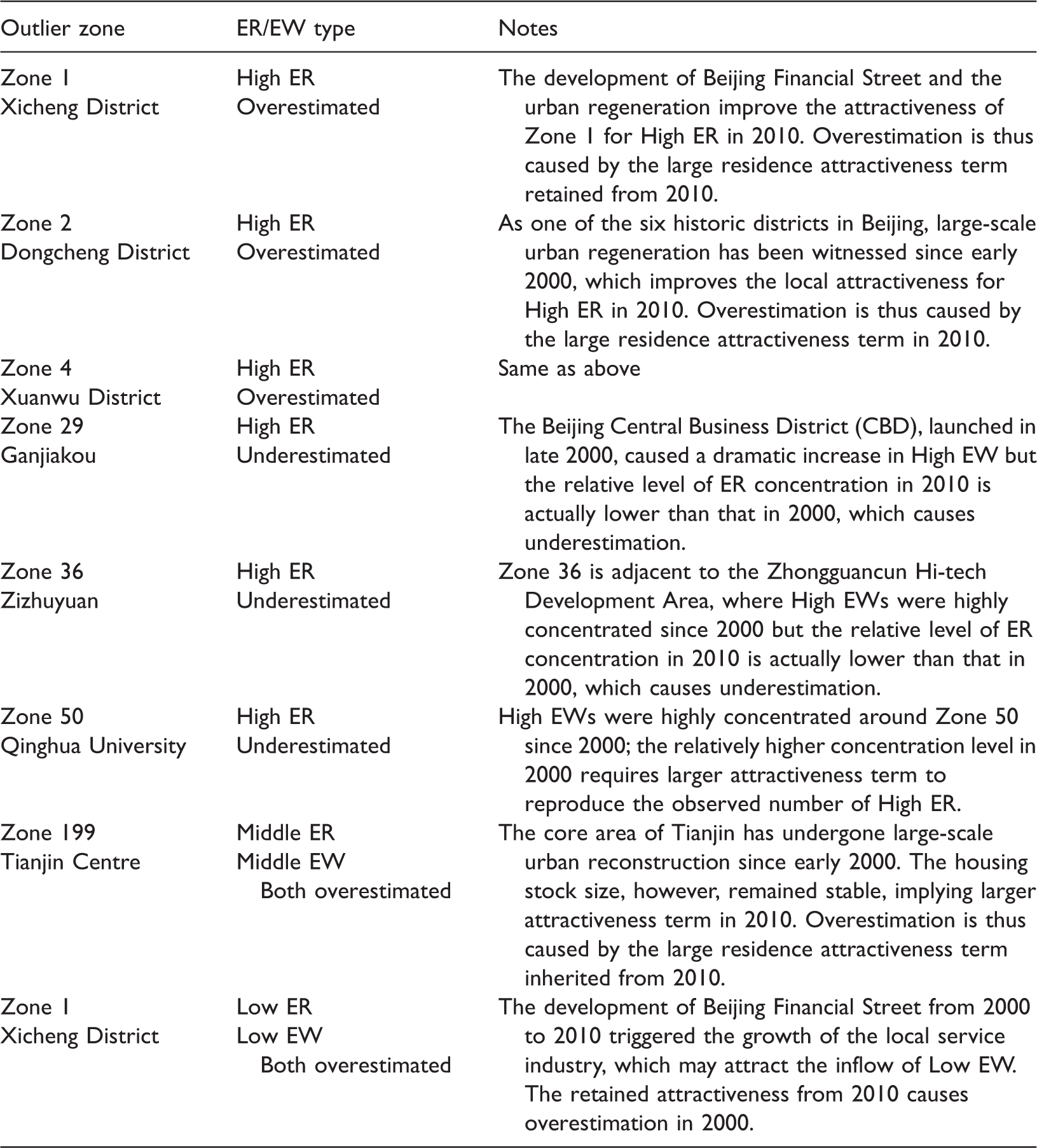
ER: employed residents; EW: employed workers.
Comparing the forward and backward forecast test, we find that some outliers are consistent in the sense that they are present in both tests. For the zones that are overestimated in the forward forecast for 2010, they are generally underestimated in the backward forecast for 2000. The inverse direction of errors implies the effectiveness of the proposed model in representing exogenous policy changes between static equilibria. We find that such policy interventions not only change the physical stock of building floorspace, but also the unobserved choice patterns (represented by the residual attractiveness term in location choice models). In model calibration, the residual attractiveness terms in location choice models come into effect and serve as a useful complement to the endogenous utility measure in order to reproduce the observed location choice patterns. The residual terms are time specific, and the model calibrated over multiple time horizons naturally involves multiple sets of such parameters. Examining the change of the residual terms over time may provide new insights into the wider impacts of stock constraints and policy interventions. In terms of modelling implications, our forward and backward forecasts show that the choice of base year is likely to have a significant impact on the outcome of model predictions. A model that is calibrated up-to-date would provide a more precise handle on model parameterizations, and thus reduce the potential modelling error in long-term forecasts.
RD model: In-sample validation
In this section, in-sample validation is conducted on the RD model for housing floorspace growth. The in-sample validation method denotes model calibration with part of the data set and model validation with the remainder. Specifically the housing growth model is first calibrated with the data set for Beijing only. This is because (1) Beijing is the key study area in the Greater Beijing city region; and (2) the data set for Beijing is verified through crosschecking data from various sources and by modellers’ accumulated local knowledge. Then the calibrated model is used to predict the housing growth for the rest of the city region (i.e. peripheral zones in Tianjin and Hebei). The predicted growth is compared with the known data.
Note that the proposed model does not model the city-region wide aggregate growth of housing. Instead we take the regional total housing growth from exogenous projections. The RD model predicts the zonal percentage share of the aggregate growth using a logit-type probabilistic model. We present the scatter plot of the modelled zonal housing growth versus the observed growth in Figure 5 for Beijing and in Figure 6 for Tianjin and Hebei. Note that the errors in Figure 5 are the regression residuals of the calibrated RD model, while Figure 6 presents the prediction errors revealed by the in-sample validation.
Housing floorspace growth model – observed vs. modelled – Beijing. Housing floorspace growth model – observed vs. modelled – Tianjin & Hebei.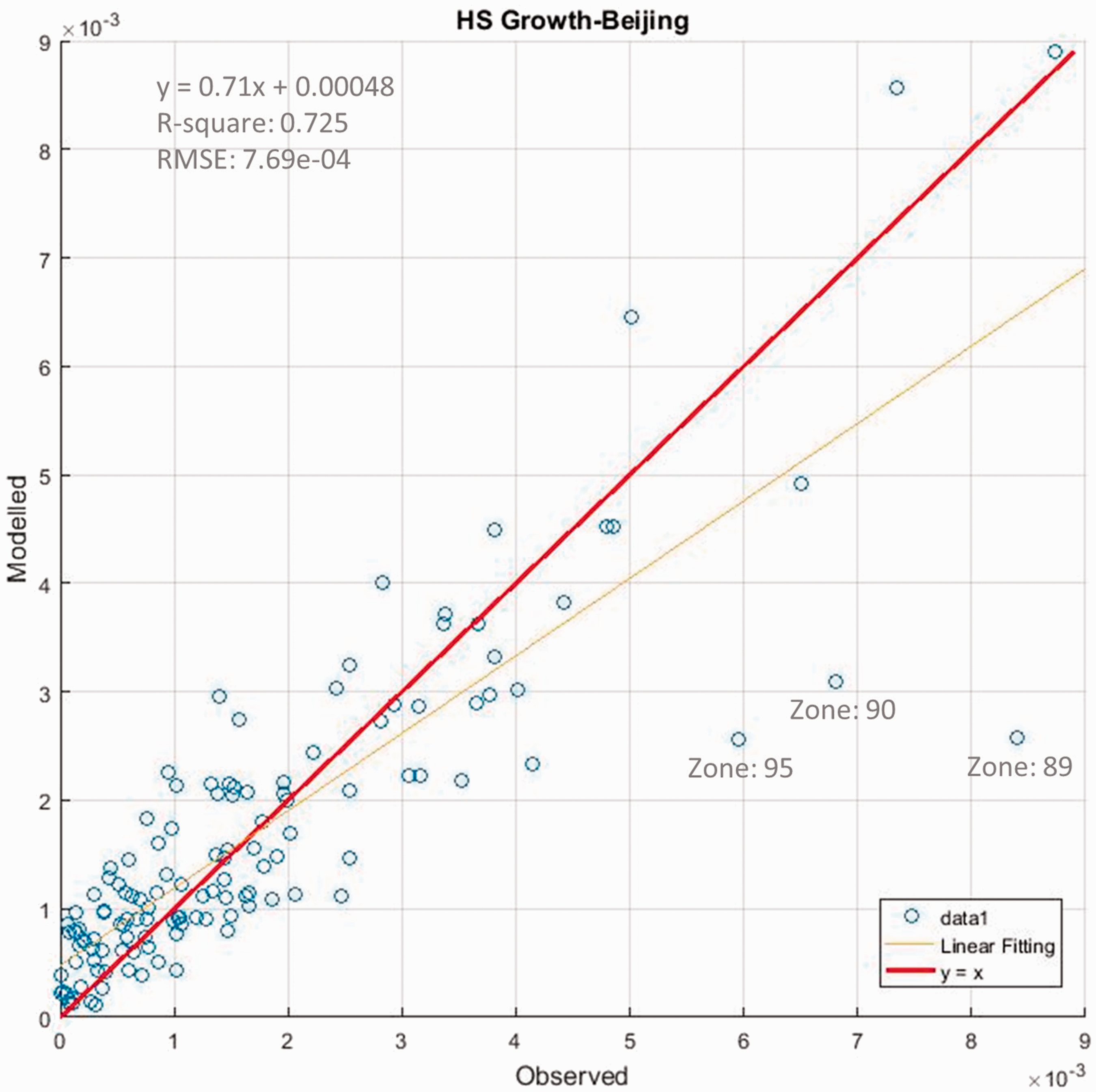
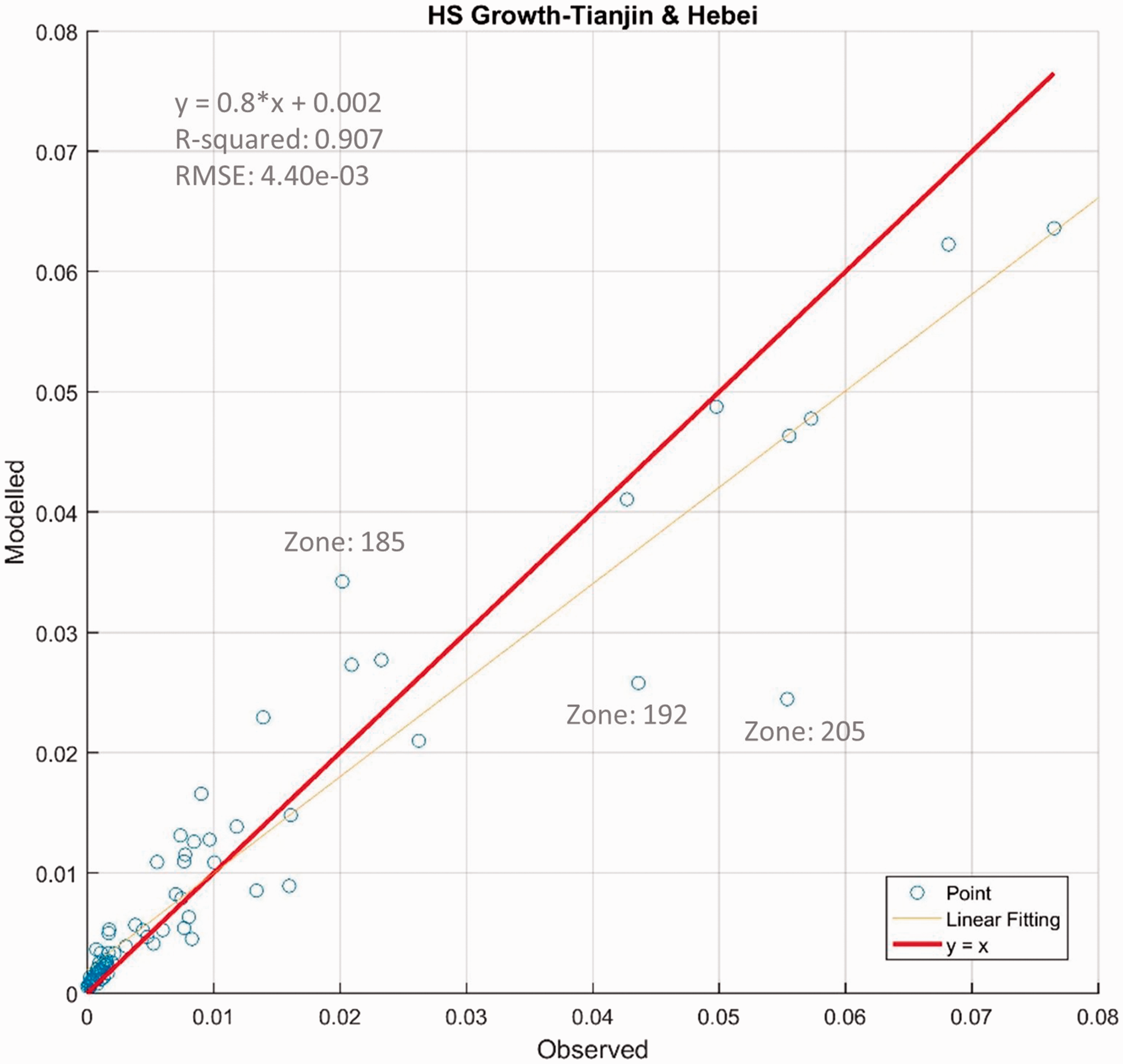
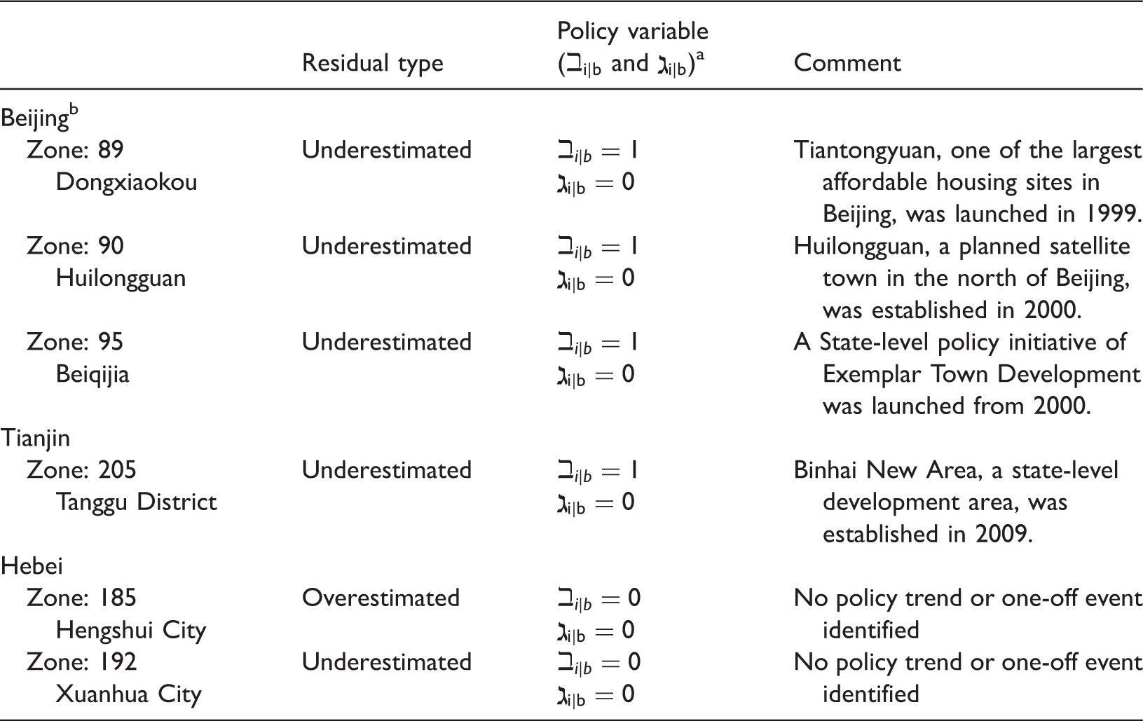
Notes on outliers – housing floorspace growth.
ℶ
The listed outliers in Beijing are excluded in the calibration process in order to prevent distorted fitting.
The investigation shows that the outliers in Figures 5 and 6 are mainly caused by exogenous policy interventions of extraordinary scale and intensity. In the RD model for housing growth, exogenous policy interventions are represented by binary dummy variables ℶ
Despite the discrepancies between the modelled and observed growth, the SE model for 2010 is calibrated using the observed floorspace data. Thus, the prediction errors of the RD models for floorspace growth do not affect the SE model for 2010. The RD models start to operate in forecast mode from 2020 onwards. In forecast mode, the model parameterization is retained, while the setting of the policy variables is subject to a scenario-specific policy scheme.
Conclusions
In this paper, we present a new LUTI model calibration and validation strategy and its application to the Greater Beijing city region. The strategy involves: (1) the calibration of the SE model for the Census years 2000 and 2010, and the calibration of the RD models for the period 2000–2010; and (2) the validation of the SE models through forward and backward forecasting and the in-sample validation of the RD models. The strategy can be used for more time horizons in the future when further observed data accumulate. The proposed modelling strategy sets a new standard for verifying and validating recursive equilibrium models.
Technically static equilibrium models can be well calibrated for a single cross section in the sense that the calibrated model is able to reproduce the observed patterns to a high accuracy. But the cross-sectional reproduction does not guarantee the predictability of the model, nor the correctness of model parameters or the data. The model validation via forward/backward forecasting thus helps to verify the stability of the model parameters. Meanwhile the exercise also helps to identify the possible calibration errors, which are difficult to detect for models with only one cross-section. By investigating the source of errors in model validation, modellers obtain a better understanding of the model’s capability in terms of what can be explained by the model and what cannot, which inspires new variables and mechanisms to be considered to improve the model representation. This learning process should become a routine feature in model calibration.
The model calibration and validation results shed a new light into the nature and precision of the RSE model. The model calibrated for the Census year 2000 is shown to be capable of generating good predictions for the year 2010 that are consistent with the observed patterns. In a hypothetical backward prediction exercise, the model calibrated for the Census year 2010 has also demonstrated the stability of the model parameters over time. This indicates that the recursive SE framework is capable of capturing the bulk of the fundamental mechanisms of the interactions among land use and transport activities through reasonably parsimonious equations.
In this paper, model validation is limited to the spatial distribution of ER and EW. In future research, model validation can be extended to other market variables, such as production output and price patterns. The model validation may also be improved through an increase in frequency. For example, in Beijing there has been a schedule of five yearly comprehensive transport surveys, which collect both land use and transport data. However, to date such data is not available to researchers outside China. In fact, many of the non-traditional statistics are likely to have disclosure restrictions attached to them, and it would be necessary to involve those who own the data sources and explore new ways to use such data in a proper manner. Increased validation frequency will also undoubtedly bring new research issues regarding model design, as more and more shorter term dynamics are revealed. These shorter term dynamics may involve complex interactions of various urban systems and are not well understood yet by modellers (Batty, 2012).
Finally, the significance of model validation goes beyond assessment of the predictive performance of any single model. It helps establish falsifiability of urban model theories through routine procedures, where the model’s predictive power is quantified with empirical evidence. The revealed gaps between the modelled and the observed indicate directions for model advancements. Small but cumulative steps could thus be made to contribute to the conviction that developing urban models is more than an act of faith, but an act of science in understanding urban complexity.
Footnotes
Declaration of conflicting interests
The author(s) declared no potential conflicts of interest with respect to the research, authorship, and/or publication of this article.
Funding
The author(s) disclosed receipt of the following financial support for the research, authorship, and/or publication of this article: Li Wan wishes to acknowledge the China Scholarship Council and the Cambridge Overseas Trust for the financial support for his doctoral study at Cambridge. Both authors wish to acknowledge the funding support for modelling methodological developments from EPSRC Global Challenge Research Fund project “Urban poverty in Chinese cities” and from a special fund of Ministry of Education of China Key Laboratory of Eco Planning & Green Building at Tsinghua University, Beijing. The usual disclaimers apply and the authors alone are responsible for views and any remaining errors.
References
Supplementary Material
Please find the following supplemental material available below.
For Open Access articles published under a Creative Commons License, all supplemental material carries the same license as the article it is associated with.
For non-Open Access articles published, all supplemental material carries a non-exclusive license, and permission requests for re-use of supplemental material or any part of supplemental material shall be sent directly to the copyright owner as specified in the copyright notice associated with the article.