Mitigating the zonal effect in modeling urban population density functions by Monte Carlo simulation

Abstract

Most empirical studies indicate that the pattern of declining urban population density with distance from the city center is best captured by a negative exponential function. Such studies usually use aggregated data in census area units that are subject to several criticisms such as modifiable areal unit problem, unfair sampling, and uncertainty in distance measure. In order to mitigate these concerns associated, this paper uses Monte Carlo simulation to generate individual residents that are consistent with known patterns of population distribution. By doing so, we are able to aggregate population back to various uniform area units to examine the scale and zonal effects explicitly. The case study in Chicago area indicates that the best fitting density function remains exponential for data in census tracts or block groups, however, the logarithmic function becomes a better fit when uniform area units such as squares, triangles or hexagons are used. The study also suggests that the scale effect remain to some extent in all area units, and the zonal effect be largely mitigated by uniform area units of regular shape.

Keywords

Monte Carlo simulation modifiable areal unit problem scale effect zonal effect urban population density function Chicago

Introduction

Since the classic study by Clark (1951), researchers have been fascinated by the regularity of declining urban population density with distance from the city center that conforms to a negative exponential function in cities across developed and developing countries (Mills and Tan, 1980; Wang and Zhou, 1999). Among the theories, the urban economic or Mills–Muth model (Mills, 1967; Muth, 1969) argues that with all jobs concentrated at the central business district (CBD), a household farther away from the CBD spends more on commuting and is compensated by more housing that is cheaper in terms of price per area unit, and the resulting population density exhibits a declining pattern with distance from the CBD. Under some assumptions (e.g. unit elasticity of housing in addition to the aforementioned monocentric employment distribution), the pattern becomes a negative exponential function. Another perspective emphasizes that the configuration of a city's street network shapes a location's attractiveness in terms of its centrality and then influences the land use intensity there, and may lead to a negative exponential population density pattern among others (Wang et al., 2011). The Garin–Lowry model (Garin, 1966; Lowry, 1964), which simulates the interaction between population and employment distributions through a city's transportation network, can also generate an exponentially-declining population density pattern given a certain basic employment pattern (Wang, 1998).

Most empirical studies on analyzing urban density patterns have used aggregated data in census or geopolitical areal units. There are several problems associated with such analysis. First, there is inaccuracy or uncertainty in measuring “distance from city center or CBD” by representing areas with their centroids. Is the centroid the geometric centroid or population center of an area? If the latter, its location varies and depends on how much detail we know about the population distribution within an area unit. This leads to another related problem, termed “modifiable areal unit problem (MAUP).” As “the areal units (zonal objects) used in many geographical studies are arbitrary, modifiable” (Openshaw, 1983), the population density pattern may also vary when different areal units are used. MAUP takes two forms: the scale effect and the zone effect. The scale effect exhibits different results when the analysis is applied to the same data but different scales in the aggregation unit. The zone (zonal) effect is observed when the scale of analysis is similar, but the shape of the aggregation unit varies.

While MAUP is considered largely intractable, there are some potential solutions to mitigate it. The issue of ecological bias inherent to polygon level data can be alleviated by inclusion of some individual-level data (Wakefield, 2007). When individual data lack, one may first model what occurs at the individual level, then analyze how the individual and group levels are related, and finally examine whether anything at the group level adds to the understanding of the relationship. The Monte Carlo simulation method meets this requirement in spatial analysis by using repeated random sampling of individual points to obtain the distribution of an unknown probabilistic entity. For example, Watanatada and Ben-Akiva (1979) used it to simulate representative individuals in an urban area in order to estimate travel demand for policy analysis. Wegener (1985) designed a Monte Carlo-based housing market model to analyze location decisions of industry and households, corresponding migration and travel patterns, and related public programs and policies. Jelinski and Wu (1996) used the technique to examine the effect of data aggregation on analysis of landscape structure as exemplified through what has become known. Poulter (1998) employed the method to assess uncertainty in environmental risk assessment and discussed related policy questions. Luo et al. (2010) used it to randomly disaggregate cancer cases from the zip code level to census blocks in proportion to the age–race composition of block population, and examined implications of spatial aggregation error in public health research. Gao et al. (2013) used it to simulate trips proportionally to mobile phone Erlang values and to predict traffic-flow distributions by accounting for the distance decay rule. Hu and Wang (2015a) used it to improve the estimate of wasteful commuting by simulating individual travelers that are consistent with the existing commute pattern. However, to our knowledge, the Monte Carlo method has not been employed to improve our estimate of urban population density functions.

Another related but distinctive issue in fitting density functions is nonrandomness of sample (Frankena, 1978). A common problem for census data is that high-density observations are many and clustered in a small area near the CBD, whereas low-density ones are fewer and scattered in remote areas. In other words, higher-density samples in shorter distance ranges are overrepresented while lower-density samples in longer distances are underrepresented. In this case, it is perhaps better termed “unfair (biased) sampling”. Some suggested using a weighted regression to mitigate the problem, for example, weighting observations in proportion to their areas (Frankena, 1978; Wang and Zhou, 1999). However, by doing so, larger-area lower-density samples are artificially valued more than others but no variability is assumed within each observation. Furthermore, a weighted regression intends to minimize the weighted residual sum of squares (RSS) not directly RSS, and the traditional goodness of fit measure such as R² is no longer valid. Therefore, some researchers favor “samples with a uniform area size” (Wang, 2015: 127).

This study examines the MAUP in analysis of the monocentric urban density pattern. The monocentric model assumes one single center and emphasizes the impact of the primary center on citywide population distribution. Researchers have increasingly recognized that in addition to the major center in the CBD, most large cities have secondary centers or subcenters, and thus are better characterized as polycentric cities (Feng et al., 2009; Ladd and Wheaton, 1991). Various population density models may be constructed under different polycentric assumptions (Heikkila et al., 1989), and the MAUP is also applicable for those polycentric models. That is beyond the scope of this research. Among large cities in the U.S., Chicago is a good example for testing the monocentric model as its largest employment center in downtown dominates other subcenters. There were more than half a million jobs within 1.5 miles from the CBD of Chicago, more than 10 times of the 2nd largest job center around the O'Hare airport (Wang, 2000). Chicago was also the city, where the classic concentric zone model was developed (Burgess, 1925).

This paper uses the Monte Carlo method to disaggregate area-based population to the individual level based on public accessible data sources. Such an approach enables us to examine population density patterns at designed uniform units. By doing so, we can explicitly assess scale and zone effects in MAUP, improve the accuracy of calibrating area centroids and thus distance measure, and generate samples of equal area size. The remainder of the paper is organized as follows. The next section discusses the study area and data sources. Section “Monte Carlo simulation of population and zonal configurations” describes technical details of Monte Carlo based population simulation and zonal configurations, and Section “Modeling urban density functions and discussion” presents the results on modeling urban density functions and discusses findings. The paper is concluded with a brief summary.

Study area and data sources

The study area is composed of seven counties in northeast Illinois (Cook, DuPage, Kane, Kendall, Lake, McHenry, and Will) as the core of Chicago CMSA (Consolidated Metropolitan Statistical Area), shown in Figure 1. The seven counties are also mostly urbanized and served by the Chicago Metropolitan Agency for Planning (CMAP), where we obtained the land use data. The area is hereafter simply referred to as Chicago. Chicago has been a popular site for urban studies as the so-called Chicago School bears its name. According to the 2010 census, the area had population about 8.2 million in an area more than 10,000 km².

Figure 1.

Study area.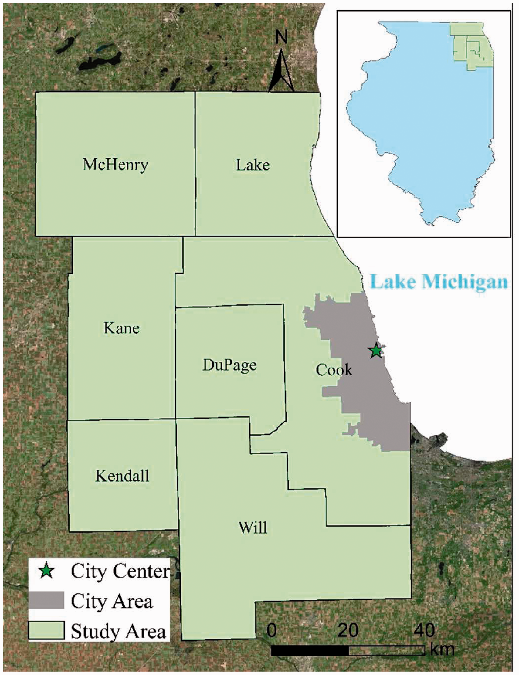

Population data at three scales (census tracts, block groups and census blocks) are extracted from the 2010 Census (www.census.gov). Census block is the smallest area unit with demographic information available from the Census. The demographic data and the TIGER-based spatial data are integrated in a GIS environment. Location for the city (CBD) center is the commonly recognized center of Chicago at the intersection of Michigan Avenue and Congress Parkway.

Another important data set is the 2010 Land Use Inventory, accessible via the CMAP Data Hub (https://datahub.cmap.illinois.gov/group/land-use-inventories). The Inventory data (version 2) are “derived directly from parcel maps” with greater accuracy in comparison to previous inventories (http://www.cmap.illinois.gov/data/land-use/inventory). This data set is critical for improving the simulation of individual level data. As the measure of population density derived from the Census is residents-based, we focus on the “residential” land use category from the CMAP data.

After extracting the residential areas, the land use layer is overlaid with the census block layer in GIS in order to identify their overlapped areas, and such an intersected areal unit is termed “residential blocks.” Residential block is a whole census block or part of a census block with its area fully defined as residential land use. As shown in Figure 2, there are three scenarios in this spatial operation:

If a residential area or multiple residential areas are wholly enclosed in a census block (Figure 2(a)), population of the census block is wholly assigned to the residential block (the case on the left side) or distributed to its enclosed residential blocks (only the areas in yellow) proportionally to their residential area sizes (the case on the right side).

If a census block or multiple census blocks are wholly enclosed in a residential area (Figure 2(b)), population remains intact (inside each block).

If a residential area is split among multiple census blocks (Figure 2(c)), the census block population is wholly assigned to a residential block when it is the only residential block inside the census block (the case on the left side), or the census block population is distributed to its enclosed residential blocks proportionally to their area sizes (the case on the right side).

Figure 2.

Relationships between residential land use and census block (census block boundary in gray, residential land use unit in yellow).

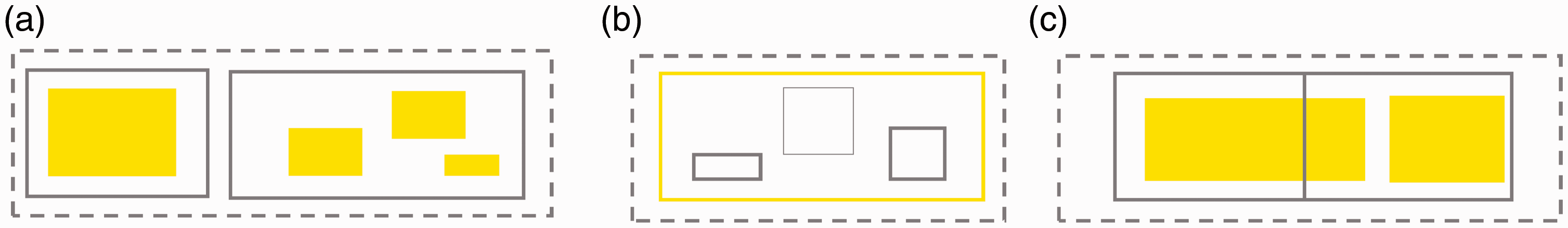
In other words, only the part (or whole) of a census block that is designated as residential land use receives allocation of population. By doing so, it utilizes the land use information to eliminate the error of distributing population to other land use types and thus improves the accuracy of population distribution simulation based on the block level census data alone.

Monte Carlo simulation of population and zonal configurations

As explained previously, population at the census block level is first allocated to the aforementioned residential blocks. For a residential block i, denote its population as n_i. The subsequent analysis simulates individual residential locations by the Monte Carlo method.

This study simulated 8,166,867 individual points to represent about the same number of residents in the study area. Specifically, the following steps were taken to simulate individuals:

Calculate the spatial extent of residential block i, denoted as [Xmin_i, Xmax_i] and [Ymin_i, Ymax_i] for the minimums and maximums for its X and Y coordinates, respectively.

Generate a random point with its X and Y coordinates within the above spatial extent. Specifically, use Monte Carlo simulation to generate a random number Xi within the range [Xmin_i, Xmax_i] and another one Yi within [Ymin, Ymax] following a uniform distribution. The two are paired as coordinates to generate a point.

Detect if a point is located within the residential block. If inside, it is retained; if outside, it is discarded.

Repeat steps 2–3 until n_i points are generated in residential block i.

Repeat steps 1–4 for all residential blocks.

Figure 3(a) uses an example to illustrate the population distribution pattern based on the census data at the census block level, and Figure 3(b) for simulated individuals if only such a data set is used. Using the same example, Figure 3(c) illustrates the adjusted population distribution by accounting for land use type, and Figure 3(d) for corresponding simulated individuals. The improvement is evident by excluding simulated individuals from non-residential areas. Here, the customized tool for “Monte Carlo Simulation of O's & D's” in Hu and Wang (2015b) was used to implement the work.

Figure 3.

Spatial distribution of (a) population in census block, (b) simulated population in census block, (c) population in residential land use areas, and (d) simulated population in residential land use areas.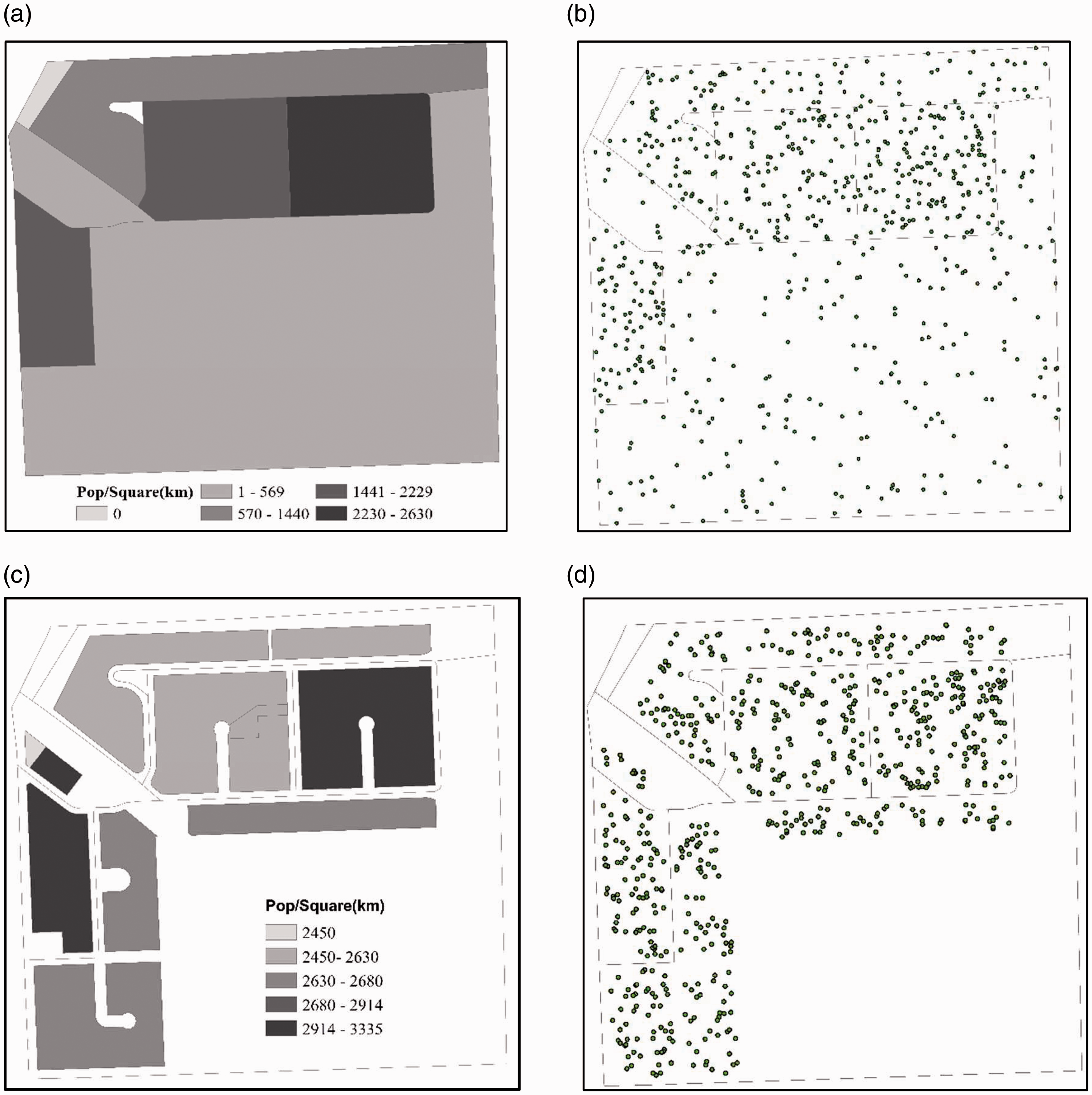

The next task is to design various configurations of analysis area units. As stated previously, it is desirable to have analysis areas of identical or similar area size. This study developed six uniform units representing three distinctive shapes (square, triangle and hexagon) and two scales so that both the zone and scale effects can be examined. The shape of area unit configuration does not necessarily imply that they are limited to a grid network of streets. In order to be comparable with the census units, the two scales were designed in a way so that their numbers of areas were similar to those of census tracts and census block groups. Census tracts and block groups are two commonly used census units in analysis of urban population density patterns, and census blocks are considered too small and have high variability of density that may not be suitable for such a study. All designed area units are uniform in area size except for those on the edge of the study area.

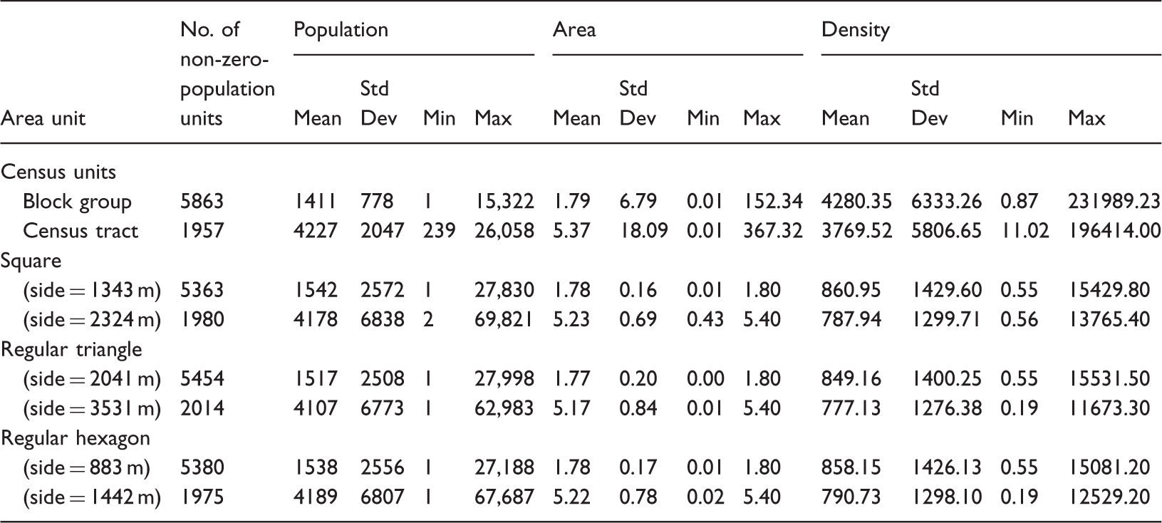
As shown in Figure 4, the layer of newly designed areas was overlaid with the layer of simulated individual residents to derive the aggregated population (and thus population density) in each area unit. For example, individual residents nested in squares, triangles and hexagons (Figure 4(a), (c) and (e)) yielded corresponding density patterns (Figure 4(b), (d) and (f)). The study area had 6307 smaller square units, 6134 smaller triangle units and 6107 smaller hexagon units, comparable to 5880 block groups; and 2054 larger square units, 2109 larger triangle units and 2094 larger hexagon units, comparable to 1964 census tracts. Table 1 presents the basic statistics for the two census units and six designed analysis units. The numbers of non-zero population area units in Table 1 are slightly lower than their total numbers. Population density in census units has a much higher variability than that in the comparable uniform area units. For example, the standard deviation of density at the block group or census tract level is about four times that of their comparable designed units.

Figure 4.

Population aggregation in uniform areal units.

Table 1.

Basic statistics for various analysis area units.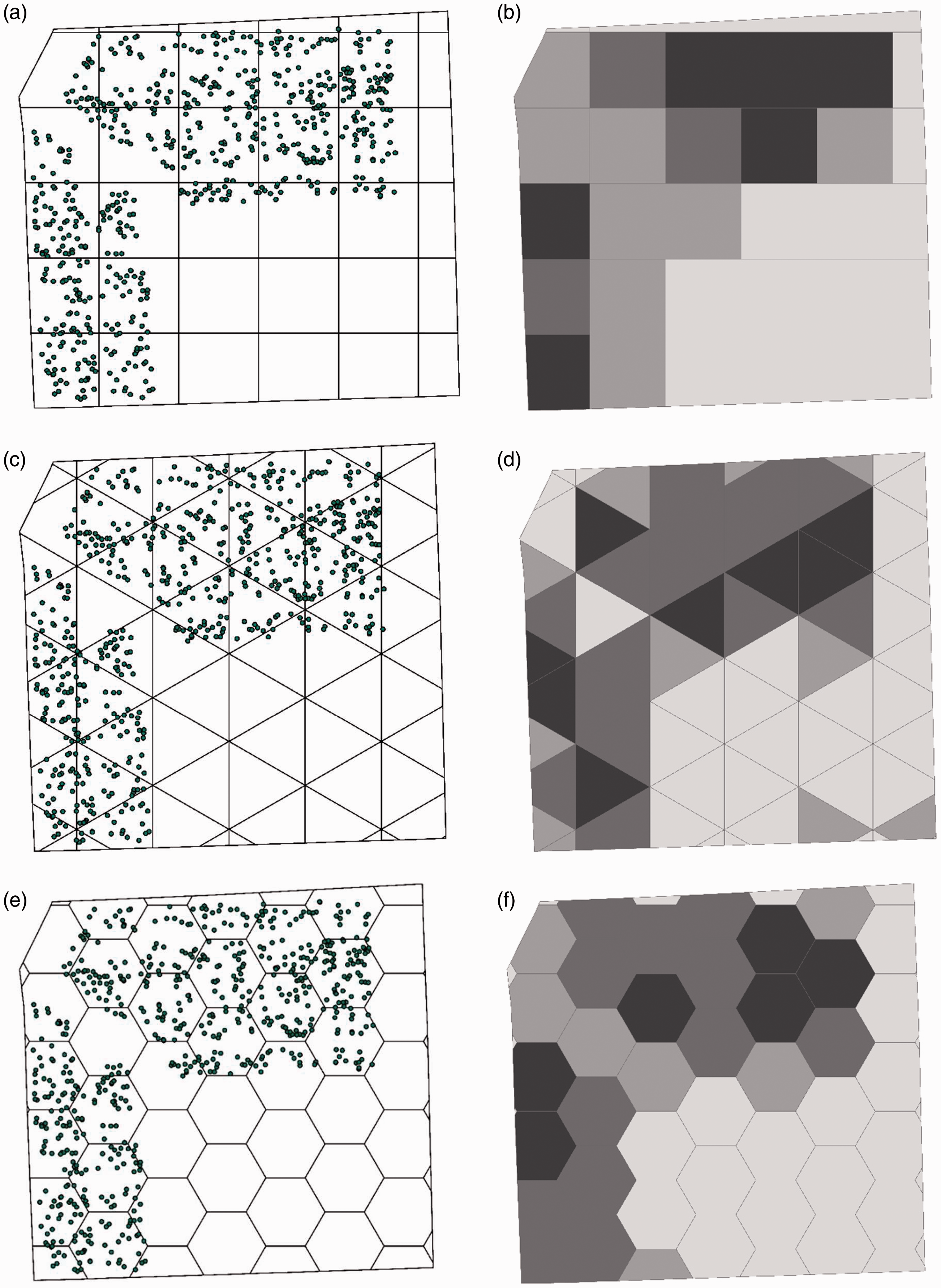

Area unit	No. of non-zero- population units	Population				Area				Density
Area unit	No. of non-zero- population units	Mean	Std Dev	Min	Max	Mean	Std Dev	Min	Max	Mean	Std Dev	Min	Max
Census units
Block group	5863	1411	778	1	15,322	1.79	6.79	0.01	152.34	4280.35	6333.26	0.87	231989.23
Census tract	1957	4227	2047	239	26,058	5.37	18.09	0.01	367.32	3769.52	5806.65	11.02	196414.00
Square
(side = 1343 m)	5363	1542	2572	1	27,830	1.78	0.16	0.01	1.80	860.95	1429.60	0.55	15429.80
(side = 2324 m)	1980	4178	6838	2	69,821	5.23	0.69	0.43	5.40	787.94	1299.71	0.56	13765.40
Regular triangle
(side = 2041 m)	5454	1517	2508	1	27,998	1.77	0.20	0.00	1.80	849.16	1400.25	0.55	15531.50
(side = 3531 m)	2014	4107	6773	1	62,983	5.17	0.84	0.01	5.40	777.13	1276.38	0.19	11673.30
Regular hexagon
(side = 883 m)	5380	1538	2556	1	27,188	1.78	0.17	0.01	1.80	858.15	1426.13	0.55	15081.20
(side = 1442 m)	1975	4189	6807	1	67,687	5.22	0.78	0.02	5.40	790.73	1298.10	0.19	12529.20

A flowchart (Figure 5) is used to summarize the above data processing procedures. The Monte Carlo simulation was repeated several times to examine possible uncertainty. The results in the density patterns in the new-configured areal units were very stable with no noticeable differences.

Figure 5.

The flowchart of data processing.

Figure 6(a) shows the population density pattern in a census unit (tracts, as an example), and Figure 6(b) in designed uniform unit (larger hexagons, as an example). The general patterns between the two are largely consistent. However, the variability in Figure 6(b) looks not as abrupt as in Figure 6(a). In addition, some zero density areas are spotted in Figure 6(b) as the hexagons contain no residential areas (only water body), but the corresponding tracts in Figure 6(a) have a small number of population there.

Figure 6.

Population density pattern in Chicago 2010: (a) census tracts and (b) uniform hexagons (side length = 1442 m).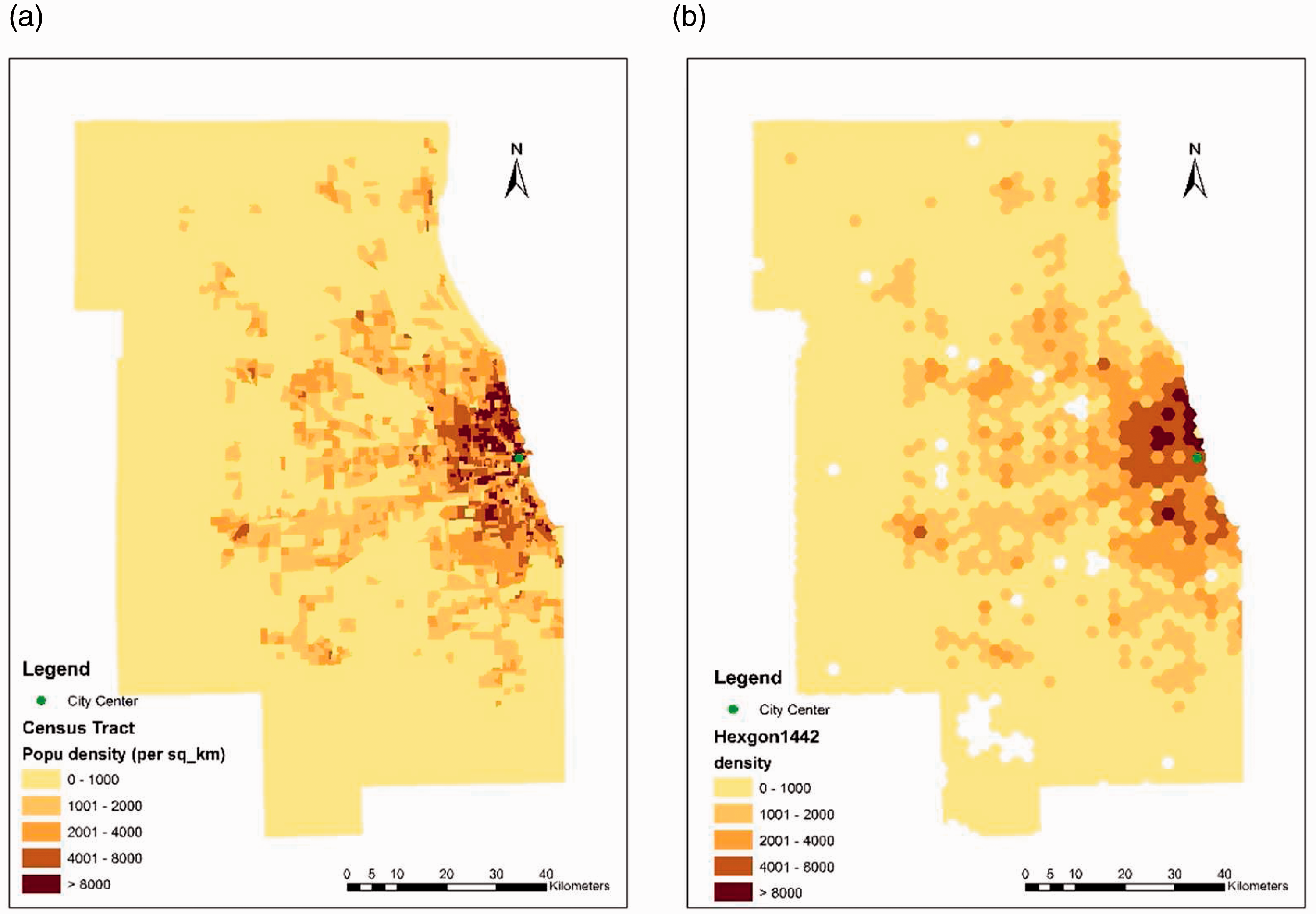

In order to measure distances from the city center, “population-weighted centroids” for block groups and census tracts were computed by utilizing the census block level data of population (Wang, 2015: 78). However, for any of the six design units, the centroid of each area was the calibrated average location for simulated individual residents within each area. For the reason discussed previously, as the simulated individual residents were a more accurate representation of population pattern than the population data at the census block level, the centroids for the design units were computed with better precision than those of census tracts or block groups. By doing so, more accurate measure of distances was achieved.

Take census tracts and hexagons (side length = 1442 m) as examples. Figure 7 shows how the numbers of observations vary by distance ranges. Indeed, there are many census tracts in short distances from the CBD (e.g. 356 tracts in 0–10 km and 501 tracts in 10–20 km), where tracts are small in area size, and the numbers decline toward longer distance ranges as tracts get larger. On the other side, the largest number of hexagons are observed in the middle distance range (350 hexagons in 60–70 km) and the numbers decline both toward the CBD (less space to be divided by fewer hexagons) and toward the urban edge (less area due to the rectangular shape of the study area).

Figure 7.

Number of observations by distance range.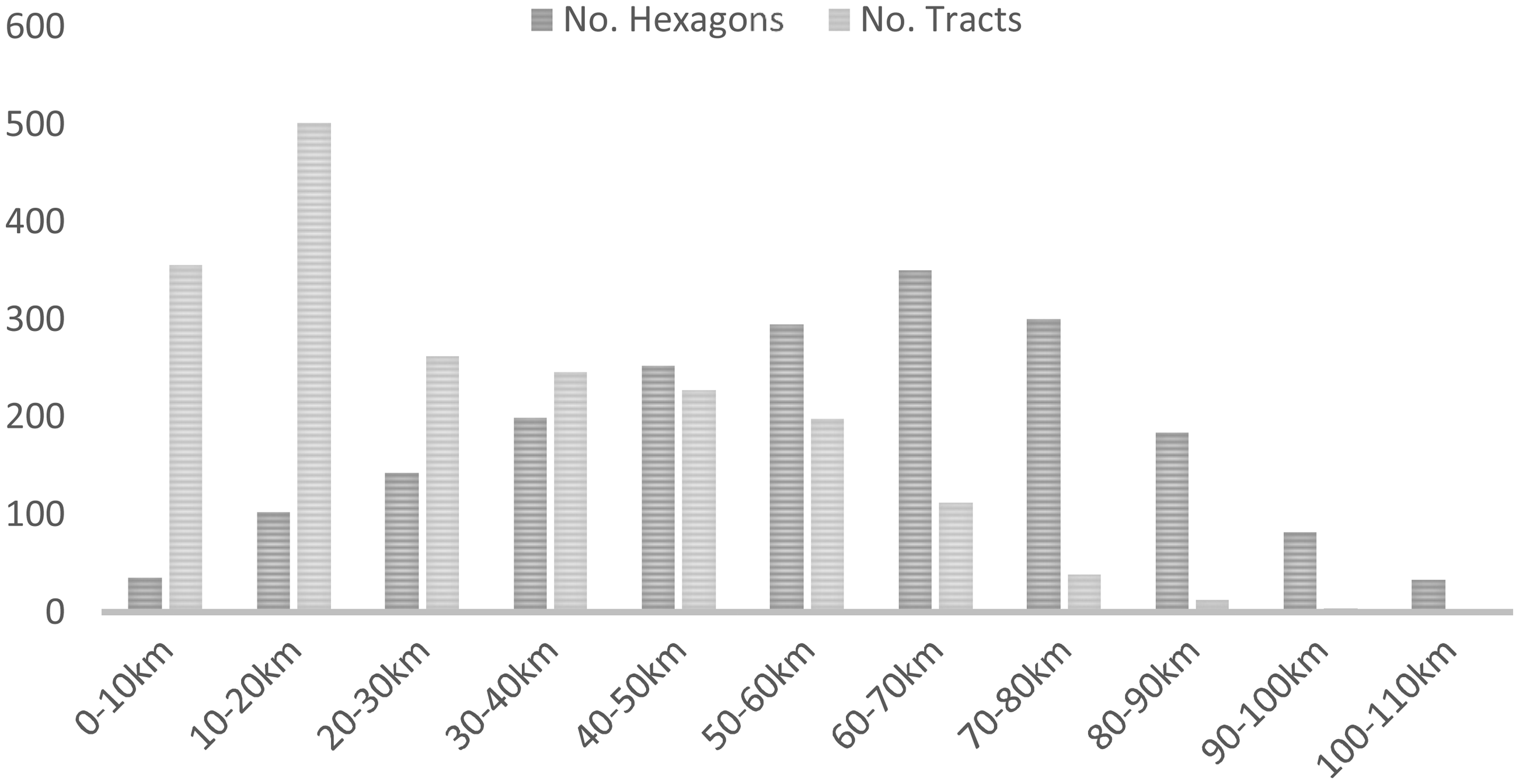

Modeling urban density functions and discussion

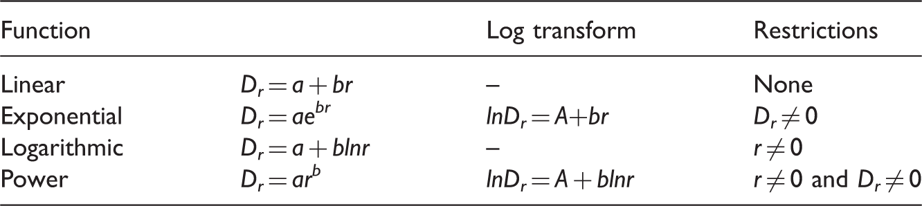
A monocentric density function captures how population density in an area D_r varies with its distance from the city center r, such as:

D_{r} = f (r)

where r is usually measured in Euclidean distance between the city center and the centroid of an area.

Table 2 summarizes four popular bivariate functions, and their logarithmic transformations if available. Newling's (1969) model (lnD_r = A+br+cr²), with one more explanatory term r², is “not comparable to the other bivariate models” (Wang, 2015: 122), and thus not analyzed here. The linear and logarithmic functions can be easily estimated by an ordinary least square (OLS) linear regression. The exponential and power functions were first transformed to linear functions by taking the logarithms on both sides, and then estimated by OLS linear regression. Note the restrictions on the data sample for preventing taking logarithms of zero. In implementation, areas with no population were excluded from regression to avoid D_r = 0; for the area where the city center falls, its centroid did not overlap with the city center in any of the eight area units used in this study, and thus no observations had r = 0.

Table 2.

Monocentric density functions used in regression analysis.

Function		Log transform	Restrictions
Linear	D _r = a + br	–	None
Exponential	D _r = ae ^br	lnD _r = A+br	D_r ≠ 0
Logarithmic	D _r = a + blnr	–	r ≠ 0
Power	D _r = ar ^b	lnD _r = A + blnr	r ≠ 0 and D_r ≠ 0

As explained previously, a weighted OLS regression was used to mitigate the problem of underrepresentation of low-density samples, and area size was used as the weight. All others were fitted by regular OLS regression. For regular OLS regression, a popular measure for a model's goodness of fit is R² (coefficient of determination), defined as the portion of a dependent variable's variation (termed total sum squared [TSS]) explained by a regression model (termed explained sum squared [ESS]); that is, R² = ESS/TSS = 1 – RSS/TSS, where RSS is residual sum of squares. R² is no longer applicable to weighted regression, however, as the identity ESS = RSS + TSS no longer holds and the residuals do not add up to 0. Here a pseudo-R² (defined similarly as 1 – RSS/TSS) was used as “an approximate measure of goodness of fit” (Wang, 2015: 124). Another index for measuring the performance of a regression is the Akaike information criterion (AIC), which captures the trade-off between the goodness of fit of a model and its complexity (i.e. the number of explanatory variables). Here, all four functions are bivariate and have the same complexity, and thus the measure of goodness of fit in R² (or pseudo-R²) is sufficient for the measure of performance. All designed area units are uniform in area size (except for a small number of areas near the borders), and thus eliminate the need of a weighted regression. The regression results by OLS are summarized in Table 3, with the highest R² or pseudo-R² highlighted in bold.

Table 3.

Regression results of population density functions by OLS.

Types of area unit and regression	Coefficients and R²	D _r = a+br	lnD _r = A+br	D _r = a+blnr	lnD _r = A+blnr
Census units (OLS)
Census Tract (n = 1957)	a (or A)	7281.16	8.93	13,672	10.73
	b	−120.28	−0.043	−3212.6	−0.99
	R ²	0.17	0.55	0.22	0.52
Census Block group (n = 5863)	a (or A)	8318.3	8.99	16,859	10.84
	b	−137.14	−0.041	−4033.9	−0.98
	R ²	0.18	0.46	0.26	0.44
Census units (weighted regression)
Census Tract (n = 1957)	a (or A)	2919.63	8.68	7956	13.77
	b	−37.90	−0.055	−1829.8	−2.09
	pseudo-R ²	0.34	0.59	0.48	0.52
Census Block group (n = 5863)	a (or A)	2904.65	8.59	7831	13.69
	b	−37.59	−0.057	−1798.1	−2.13
	pseudo-R ²	0.27	0.52	0.38	0.43
Designed uniform units (OLS)
Square (2324 m, n = 1980)	a (or A)	2892.0	9.14	7728	15.30
	b	−37.30	−0.071	−1771.8	−2.60
	R ²	0.41	0.51	0.58	0.42
Square (1343 m, n = 5363)	a (or A)	3037.34	9.02	8103	15.07
	b	−39.28	−0.069	−1858.0	−2.54
	R ²	0.37	0.46	0.52	0.39
Triangle (3531 m, n = 2014)	a (or A)	2857.53	9.11	7784	15.42
	b	−36.65	−0.070	−1785.9	−2.62
	R ²	0.42	0.51	0.60	0.43
Triangle (2041 m, n = 5454)	a (or A)	3005.7	8.97	8070	15.04
	b	−38.86	−0.068	−1851.6	−2.53
	R ²	0.38	0.46	0.54	0.39
Hexagon (1442 m, n = 1975)	a (or A)	2918.81	9.12	7879	15.36
	b	−37.54	−0.070	−1807.0	−2.61
	R ²	0.42	0.50	0.59	0.42
Hexagon (883 m, n = 5380)	a (or A)	3039	8.97	8099	15.04
	b	−39.23	−0.069	−1856.4	−2.53
	R ²	0.38	0.45	0.53	0.38

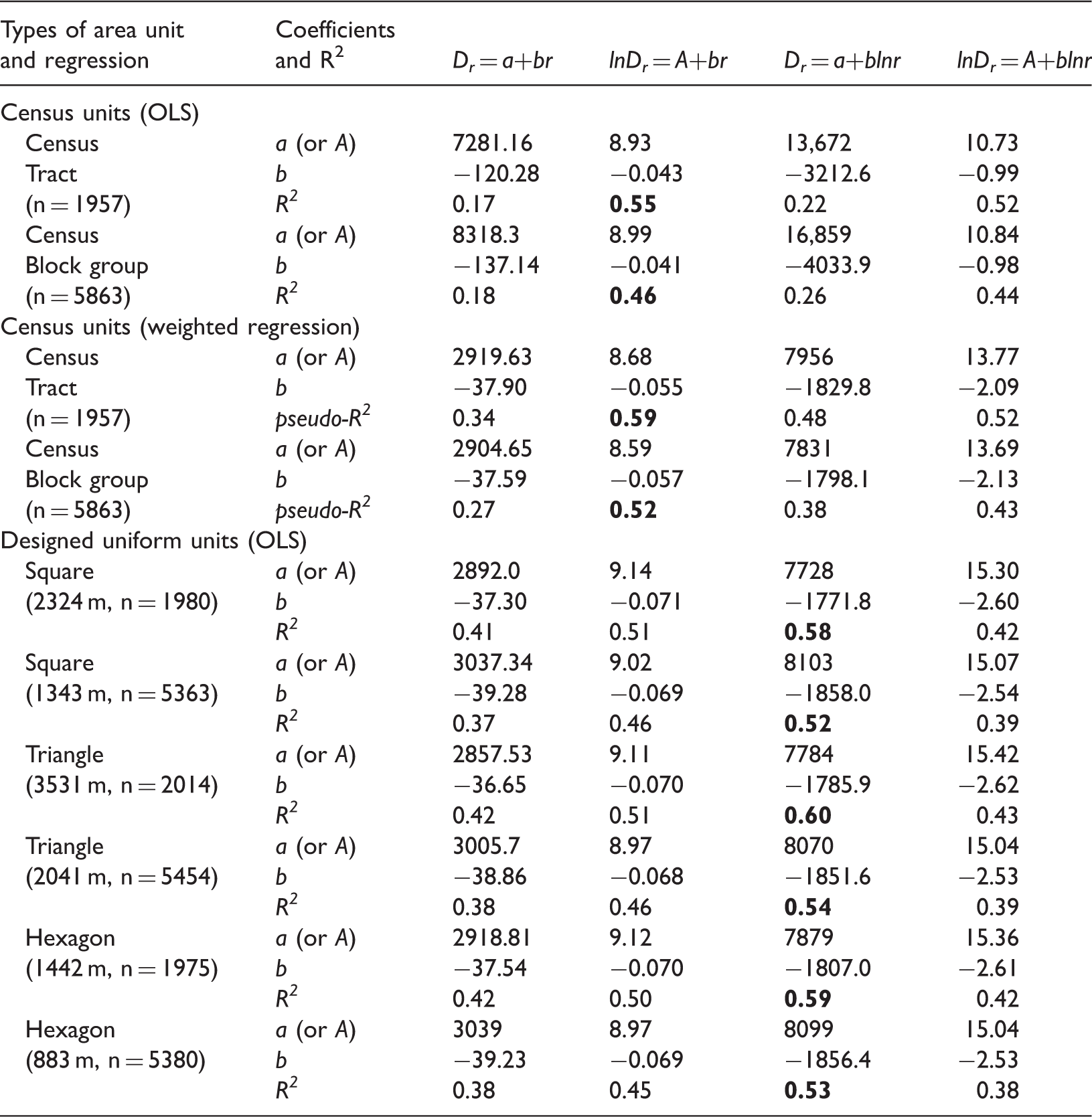
Note: A number in bold indicates the highest R2 or pseudo-R2 (i.e., best-fitting function) in each case.

Another statistical issue concerns the spatial dependence (autocorrelation) of the sample in fitting the urban density functions, and calls for the use of spatial regression (Griffith and Wong, 2007). There are two common spatial regression models: spatial lag and spatial error models. The former adds the spatial lag of the dependent variable as an extra explanatory variable in the regression; and the latter considers the error term as autoregressive and derives an independent second error term by controlling the effect of the spatial lag of the original error term. This research used GeoDa (http://geodacenter.github.io/) to implement both spatial regression models by the maximum likelihood method. By default, GeoDa uses the Euclidean distance matrix between observations to define the spatial weights. As stated previously, population-weighted centroids are used to represent locations of area units for better accuracy. Since the two models yielded the results that were largely consistent with each other, Table 4, also with the highest R² or pseudo-R² highlighted in bold, only presents the results by the spatial lag model.

Table 4.

Regression results of population density functions by the spatial lag model.

Types of area unit	Coefficients and R²	D _r = a+br	lnD _r = A+br	D _r = a+blnr	lnD _r = A+blnr
Census units (spatial lag)
Census Tract (n = 1957)	a (or A)	4194.34	2.69	8725	3.07
	b	−69.62	−0.01	−2056.7	−0.28
	Spatial lag	0.46	0.71	0.40	0.72
	R ²	0.27	0.74	0.28	0.74
Census Block group (n = 5863)	a (or A)	2523.14	2.93	5850	3.41
	b	−41.25	−0.012	−1404.2	−0.29
	Spatial lag	0.75	0.68	0.71	0.69
	R ²	0.52	0.67	0.52	0.67
Designed uniform units (spatial lag)
Square (2324 m, n = 1980)	a (or A)	2036.11	6.71	5813	10.76
	b	−26.36	−0.05	−1335.0	−1.85
	Spatial lag	0.32	0.28	0.28	0.33
	R ²	0.57	0.62	0.65	0.59
Square (1343 m, n = 5363)	a (or A)	970.69	3.22	3279	4.82
	b	−12.55	0.64	−751.3	−0.81
	Spatial lag	0.67	−0.02	0.58	0.68
	R ²	0.69	0.70	0.70	0.70
Triangle (3531 m, n = 2014)	a (or A)	927.58	3.66	3376	5.58
	b	−11.90	−0.028	−775.4	−0.95
	Spatial lag	0.68	0.60	0.57	0.64
	R ²	0.75	0.73	0.76	0.73
Triangle (2041 m, n = 5454)	a (or A)	807.52	3.02	2798	4.56
	b	−10.43	−0.023	−642.0	−0.77
	Spatial lag	0.73	0.66	0.65	0.69
	R ²	0.73	0.70	0.74	0.70
Hexagon (1442 m, n = 1975)	a (or A)	698.48	2.65	2641	3.83
	b	−8.99	−0.02	−605.8	−0.65
	Spatial lag	0.75	0.71	0.66	0.75
	R ²	0.767	0.75	0.77	0.75
Hexagon (883 m, n = 5380)	a (or A)	703.37	2.48	2467	3.71
	b	−9.09	−0.019	−565.3	−0.63
	Spatial lag	0.76	0.72	0.69	0.75
	R ²	0.73277	0.72	0.73	0.72

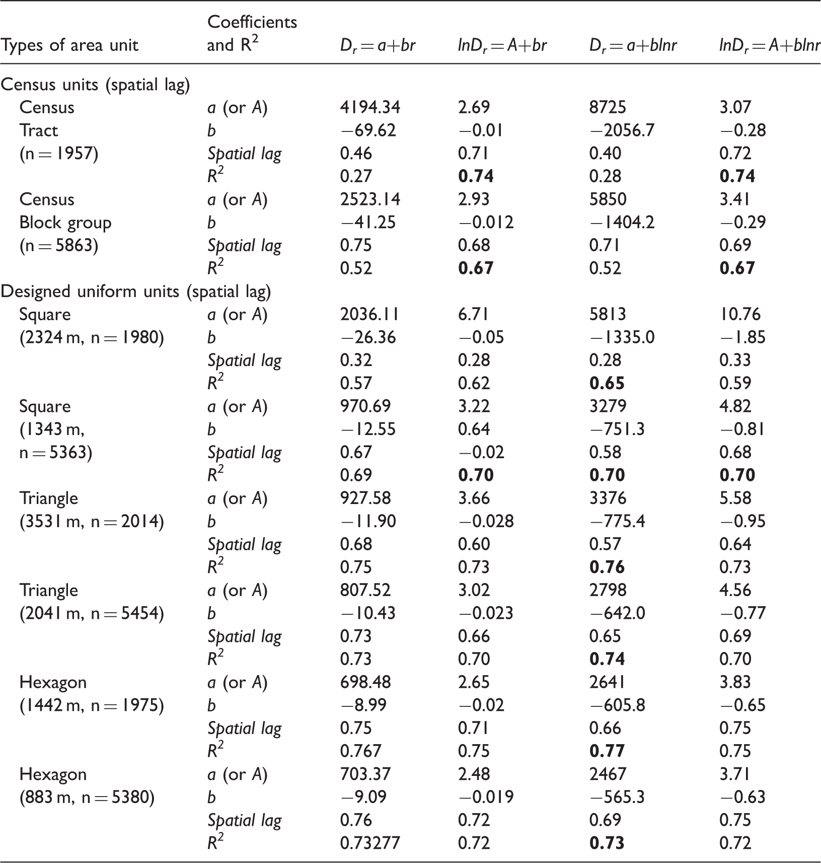
Note: A number in bold indicates the highest R2 or pseudo-R2 (i.e., best-fitting function) in each case.

Several findings are highlighted below:

Based on R² in Table 3 (either regular or weighted OLS regression), the best fitting function is exponential for census units, but logarithmic for designed uniform units; and the finding is consistent across two census units and across six uniform units. In other words, as further illustrated in Figure 8(a) and (b), respectively, (a) for census units, population density tends to decline exponentially when distance from the CBD increases linearly, and (b) for designed units, population density tends to decline linearly when distance from the CBD increases exponentially. The order of fitting power for the four functions is: “exponential > power > logarithmic > linear” for census units, and “logarithmic > exponential > power > linear” for uniform units. This difference shows a major zonal effect between census units and designed uniform units.

The above finding from OLS regression is largely confirmed by the results from the spatial regression (specifically spatial lag model) as reported in Table 4. The best fitting function remains exponential for the two census units, and logarithmic for the six uniform units, although the advantages over alternative functions in terms of R² are narrowed. For example, the power function comes as good as the exponential for both census units; and the R² values for small square areas (side = 1343 m) are also identical for the exponential, logarithmic and power functions (i.e. negligible difference). Given the consistency in the results between the OLS and spatial regression models, the following discussion emphasizes on the results from Table 3.

Another noticeable difference between census units and uniform units is the regression coefficients. Based on the exponential function results (the best for census units and the 2nd best for uniform units), census units generally yield flatter gradients (b) than uniform units. For both census units, the weighted regression returns also a steeper slope than the OLS regression. In other words, the density gradients in the exponential function are stepper in the uniform units than those in the census units by weighted regression, which are steeper than those in the census units by OLS. As explained in the previous section, low-density census units are fewer with larger area size and farther distance from the city center. In contrast, there are much more low-density uniform units in about the same area, which pushes the tail of the fitted curve further down and thus a steeper gradient. The weighted regression exerts a similar effect as it assigns larger weights to larger-area low-density census units, and thus yields a higher gradient than that in census units by OLS, but not to the degree of using designed units with a uniform area size (and thus its gradient value is between census units by OLS and uniform units). The pattern is alerted for uniform units to a degree that is better fitted by a logarithmic function. The finding of a steeper density gradient in equal or comparable area size than census units is consistent in both OLS and spatial regressions from Tables 3 and 4.

On the zonal effect within the designed units, the regression results are largely consistent across squares, triangles and hexagons in a similar scale. For example, based on the best-fitting logarithmic function, the goodness of fit (R²) is nearly identical in larger units (0.58–0.60) or in smaller units (0.52–0.54) across three shapes; and the coefficients vary in narrow ranges (i.e. 7728–7879 and 8070–8103 for the intercept in the 3 larger and 3 smaller units, respectively; and 1771.8–1807.0 and 1851.6–1858.0 for the slope in the 3 larger and 3 smaller units, respectively). It is reasonable to conclude that the zonal effect is minimal or negligible in the designed uniform areal units.

In terms of scale effect, the fitting power is higher in larger areal units in either census units (census tracts compared to block groups) or designed units (across squares, triangles or hexagons). This is understandable as some of the variability of population density is smoothed out in larger unit with fewer observations to explain by a regression model.

Again on the scale effect, based on the best fitting exponential function on census units, the OLS yields a slightly steeper slope in larger unit (census tracts) than smaller one (block groups) while the weighted regression reverses the trend (i.e. flatter gradient in census tracts than block groups). For designed units, larger units yield slightly flatter gradients than smaller units in the exponential function, but a reversed trend by the best fitting logarithmic function. As the differences are minor and the results by various methods are conflicting, we refrain from further discussion.

To recap the above observations, the results from the census units and designed uniform units differ in (1) the best fitting density function form and (2) the density gradient when using the same function. On the former, it suggests that the exponential function, often found as the best fitting function in empirical studies, could be an artifact of data reporting based on arbitrarily defined area units. On the latter, a city with its analysis unit defined as equal or comparable area size is likely to produce a steeper density gradient than using census units. In addition, the scale effect remains an issue regardless of census units or designed uniform units, but it has not reached a point to alter aforementioned major findings (e.g. the best fitting function within census units or uniform units, poorer fitting power in data of smaller areas). The zonal effect is largely mitigated across various configurations of uniform regular shapes.

Figure 8.

Population density vs. distance: (a) census tracts (y-axis in exponential scale), (b) uniform hexagons (side length = 1442 m; x-axis in exponential scale).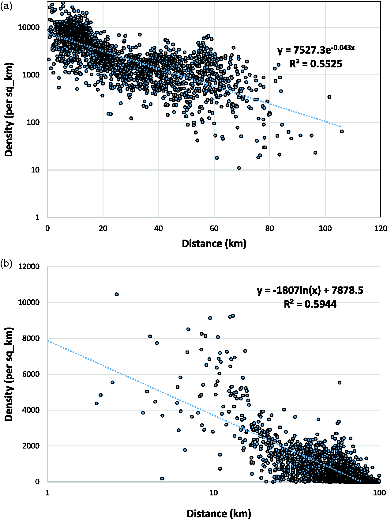

What is the best fitting density function? Does the question even matter? In terms of the theoretical foundation for the negative exponential function, the Mills–Muth model provides the most convincing reasoning based on economic theories. However, both assumptions for the model such as the monocentric structure in employment distribution and unit elasticity for housing market are not completely supported by empirical studies (McDonald, 1989). In other words, the drive to pursue a theoretical model for explaining the exponential urban density pattern is ill advised. One has to look for alternative models that are more flexible and accommodative of complexity of the real-world cities. For example, simulations based on the Garin–Lowry model suggest that the density pattern in a city may be best captured by a function different from “exponential” or even polycentric when the employment distribution or the transport network changes (Wang, 1998).

Conclusion

Researchers have long been fascinated by the regularity of population density pattern that is best captured by a negative exponential function in cities across countries at different levels of economic development. In the meantime, empirical studies have relied on data aggregated in various area units such as census or administrative units, and are subject to criticisms including MAUP, unfairness of sampling, and inaccuracy or uncertainty in distance measure by using centroids to areas. This paper attempts to mitigate these concerns by simulating individual resident locations. It is achieved by Monte Carlo simulation that utilizes the census data and other accessory data (in our case, land use inventory data derived from parcel maps) to randomly generate individuals that are consistent with known patterns of population distribution. The simulated data enables us to aggregate population back to area units of any scale in any shape so that the scale effect and the zonal effect can be examined explicitly. For our interest, uniform regular shapes are designed to alleviate the issue of unfair sampling. When an area is represented as the average location of individuals within the area, it yields a more accurate centroid to facilitate the distance calibration.

Case studies from cities around the world (including this one in Chicago) indicate that the best fitting density function usually is exponential. Many take this as a fact and a foundation for subsequent analyses. For example, Chen (2010) derived a latent fractal structure in a Chinese city based on a generalized exponential urban density function; and Bertaud and Malpezzi (2014) attempted to explain the variability of the density gradient derived from this function across different countries, markets, sizes, histories, geographic settings and so on. This research suggests that such a finding could be entirely attributable to the areal units (often census units such as census tract or block group in the U.S., enumeration district or output area in the U.K., or geopolitical units such as jiedaoban or juweihui in China). When uniform area units such as squares, triangles or hexagons are used (as preferred by some statisticians), the exponential function may not yield the best fit. In this case study, it is surpassed by the logarithmic in fitting power.

This finding is significant for at least two reasons. On the empirical side, the commonly observed exponential urban density pattern may be an artifact of census data reported in artificially defined census units. As cities become increasingly complex (e.g. toward polycentricity, suburbanization and perhaps fragmentation), it is no surprise that the fitting power by the exponential function has declined over time (Feng et al., 2009; McDonald, 1989; Wang and Zhou, 1999). Even when the exponential function is the best-fitting one for a city (as it is the case for Chicago based on census units), it is possibly a product of using census geography as analysis unit. In terms of its theoretical implication, as the monocentric economic model remains the dominant theory in explaining such a pattern, alternative models need to be considered to better explain the complexity of the real-world cities. The case study also suggests that the scale effect, likely inherent in such area-based analysis, remains to some extent, and the zonal effect be very much mitigated by designing uniform area units of regular shape. Given the convenience of implementing the Monte Carlo simulation method (e.g. using the program cited in this paper), replication of our approach in other cities is welcomed to test its validity.

Future work may extend the research in several directions. First, the current Monte Carlo simulation assumes a uniform distribution of individual resident locations within a “residential block” (though random). More accurate simulation may utilize data of ancillary variables (e.g. vegetation index, nighttime light, road network) to further differentiate possible density variability within a small area and improve the simulation (e.g. Li and Weng, 2005; Mellander et al., 2015; Xie, 1995). Secondly, one may also use agent-based modeling such as the spatial microsimulation (Lovelace and Dumont, 2016) to simulate individual residents within census areas or geopolitical units by utilizing national surveys of aspatial individual-level data and aggregated data. Thirdly, the density function approach is a simplistic yet elegant model of urban population settlement patterns. Various realistic and complex elements can be introduced to examine the impact of spatial impedance on urban structure. For instance, one may use travel time through the real transport networks by multiple modes to design a comprehensive measure of spatial impedance in place of the simple Euclidean distance measure. Furthermore, as discussed previously, this paper focuses on examining the zonal effect in a monocentric framework, and future work can analyze how the polycentric models may also be affected by various configurations of zones.

Footnotes

Declaration of conflicting interests

The author(s) declared no potential conflicts of interest with respect to the research, authorship, and/or publication of this article.

Funding

The author(s) received no financial support for the research, authorship, and/or publication of this article.

Fahui Wang is James J Parsons professor in Department of Geography & Anthropology, Louisiana State University. His research interests include applications of GIS and computational methods in urban and regional planning, transportation, and public health.

Cuiling Liu is a PhD student in Department of Geography & Anthropology, Louisiana State University. Her interests include GIS, spatial analysis and applications in human geography.

Yaping Xu is a PhD student in Department of Geography & Anthropology, Louisiana State University. His interests include GIS, remote sensing and their applications.

References

Bertaud A and Malpezzi S (2014) The spatial distribution of population in 57 world cities: The role of markets, planning, and topography. Draft paper online. Available at: http://coller.tau.ac.il/sites/nihul.tau.ac.il/files/media_server/Recanati/management/elrov/june2014_symposium/Malpezzi.pdf (accessed 22 August 2017).

Burgess

(1925) The growth of the city. In: Park

Burgess

Mackenzie

(eds) The City, Chicago: University of Chicago Press, pp. 47–62.

Chen

Y-G

(2010) A new model of urban population density indicating latent fractal structure. International Journal of Urban Sustainable Development 1: 89–110.

Clark

(1951) Urban population densities. Journal of Royal Statistical Society 114: 490–494.

Feng

Wang

Zhou

Y-X

(2009) The spatial restructuring of population in metropolitan Beijing: Toward polycentricity in the post-reform era. Urban Geography 30: 779–802.

Frankena

(1978) A bias in estimating urban population density functions. Journal of Urban Economics 5: 35–45.

Gao

Wang

Gao

et al. (2013) Understanding urban traffic-flow characteristics: A rethinking of betweenness centrality. Environment and Planning B 40: 135–153.

Garin

(1966) A matrix formulation of the Lowry model for intrametropolitan activity allocation. Journal of the American Institute of Planners 32: 361–364.

Griffith

Wong

(2007) Modeling population density across major US cities: A polycentric spatial regression approach. Journal of Geographical Systems 9: 53–75.

10.

Heikkila

Gordon

Kim

et al. (1989) What happened to the CBD-distance gradient? Land values in a polycentric city. Environment and Planning A 21: 221–232.

11.

Wang

(2015a) Decomposing excess commuting: A Monte Carlo simulation approach. Journal of Transport Geography 44: 43–52.

12.

Wang

(2015b) Monte Carlo method and its application in urban traffic simulation. In: Wang

(ed.) Quantitative Methods and Socio-Economic Applications in GIS, Boca Raton, FL: CRC Press, pp. 259–277.

13.

Jelinski

(1996) The modifiable areal unit problem and implications for landscape ecology. Landscape Ecology 11: 129–140.

14.

Ladd

Wheaton

(1991) Causes and consequences of the changing urban form: Introduction. Regional Science and Urban Economics 21: 157–162.

15.

Weng

(2005) Using Landsat ETM + imagery to measure population density in Indianapolis, Indiana, USA. Photogrammetric Engineering & Remote Sensing 71: 947–958.

16.

Lovelace

Dumont

(2016) Spatial Microsimulation with R, Boca Raton, FL: CRC Press.

17.

Lowry

(1964) A Model of Metropolis, Santa Monica, CA: Rand Corporation.

18.

Luo

McLafferty

Wang

(2010) Analyzing spatial aggregation error in statistical models of late-stage cancer risk: A Monte Carlo simulation approach. International Journal of Health Geographics 51.

19.

McDonald

(1989) Econometric studies of urban population density: A survey. Journal of Urban Studies 31: 201–218.

20.

Mellander

Lobo

Stolarick

et al. (2015) Night-time light data: A good proxy measure for economic activity?. PLoS ONE 10(10): e0139779.

21.

Mills

(1967) An aggregative model of resource allocation in a metropolitan area. The American Economic Review 57(2): 197–210.

22.

Mills

Tan

(1980) A comparison of urban population density functions in developed and developing countries. Urban Studies 17(3): 313–321.

23.

Muth

(1969) Cities and Housing, Chicago: University of Chicago.

24.

Newling

(1969) The spatial variation of urban population densities. Geographical Review 59: 242–252.

25.

Openshaw

(1983) The Modifiable Areal Unit Problem, Norwick: Geo Books.

26.

Poulter

(1998) Monte Carlo simulation in environmental risk assessment: Science, policy and legal issues. Risk: Health Safety and Environment 9: 7–26.

27.

Wakefield

(2007) Disease mapping and spatial regression with count data. Biostatistics 8(2): 158–183.

28.

Wang

(1998) Urban population distribution with various road networks: A simulation approach. Environment and Planning B: Planning and Design 25: 265–278.

29.

Wang

(2000) Modeling commuting patterns in Chicago in a GIS environment: A job accessibility perspective. Professional Geographer 52: 120–133.

30.

Wang

(2015) Quantitative Methods and Socio-Economic Applications in GIS, Boca Raton, FL: CRC Press.

31.

Wang

Antipova

Porta

(2011) Street centrality and land use intensity in Baton Rouge, Louisiana. Journal of Transport Geography 19: 285–293.

32.

Wang

Zhou

(1999) Modeling urban population densities in Beijing 1982–90: Suburbanisation and its causes. Urban Studies 36: 271–287.

33.

Watanatada

Ben-Akiva

(1979) Forecasting urban travel demand for quick policy analysis with disaggregate choice models: A Monte Carlo simulation approach. Transportation Research Part A: General 13(4): 241–248.

34.

Wegener

(1985) The Dortmund Housing Market Model: A Monte Carlo simulation of a regional housing market. Lecture Notes in Economics and Mathematical Systems 239: 144–191.

35.

Xie

(1995) The overlaid network algorithms for areal interpolation problem. Computer, Environment and Urban Systems 19: 287–306.