Assessing nighttime lights for mapping the urban areas of 50 cities across the globe

Abstract

Nighttime data from the Defense Meteorological Satellite Program Operational Linescan System have been widely used to map urban/built-up areas (hereafter referred to as “built-up area”), but to date there has not been a geographically comprehensive evaluation of the effectiveness of using nighttime lights data to map urban areas. We created accurate, convenient, and scalable grid cells based on Defense Meteorological Satellite Program/Operational Linescan System nighttime light pixels. We then calculated the density of Landsat-derived built-up areas within each grid cell. We explored the relationship between Defense Meteorological Satellite Program/Operational Linescan System nighttime lights data and the density of built-up areas to assess the utility of nighttime lights for mapping urban areas in 50 cities across the globe. We found that the brightness of nighttime lights was only in moderate agreement with the density of built-up areas; moreover, correlations between nighttime lights and Landsat-derived built-up areas were weak. Even in relatively sparsely populated urban regions (where the density of the built-up area is less than 20%), the highest correlation coefficient (R²) was only 0.4. Furthermore, nighttime lights showed lighted areas that extended beyond the area of large cities, and nighttime lights reduced the area of small cities. The results suggest that it is difficult to use the regression model to calibrate the Defense Meteorological Satellite Program/Operational Linescan System nighttime lights to fit urban built up areas.

Keywords

Defense Meteorological Satellite Program nighttime lights cities soil sealing Landsat

Introduction

Nighttime data from the Defense Meteorological Satellite Program (DMSP) Operational Linescan System (OLS) have been widely used to monitor and analyze human activities and natural phenomena, such as in assessments of urban areas (Elvidge et al., 1997; He et al., 2014; Imhoff et al., 1997; Stathakis et al., 2015; Tan, 2017; Zhou et al., 2014), estimates of energy use and carbon emissions (Fragkias et al., 2016; Oda and Maksyutov, 2011), and forecasts of gross domestic product (Liu et al., 2016; Zhao et al., 2017), and in combination with detailed census data and land use data to establish a correlation with population density at fine spatial scales (Bagan and Yamagata, 2015). Doll (2008) presents a comprehensive discussion of the collection, use, and pitfalls of the nighttime lights dataset. The Suomi National Polar-orbiting Partnership (Suomi NPP) satellite was launched in 2011, and the onboard Visible Infrared Imaging Radiometer Suite (VIIRS) sensor began collecting data in day/night bands (Elvidge et al., 2013; Miller et al., 2012; Stathakis, 2015). The VIIRS product provides several key improvements over DMSP/OLS data, and the procedures for generating VIIRS night-time lights involve a series of filtering steps to exclude low-quality data and extraneous features (Elvidge et al., 2017). However, VIIRS nighttime lights datasets do not meet the time-series requirements of certain studies (Levin and Phinn, 2016). Thus, DMSP/OLS nighttime lights data remain the dominant source of nighttime lights observations.

Since 1992, the nighttime lights annual composites dataset from the DMSP/OLS nighttime lights data has been processed and distributed annually with a spatial resolution of 30 arc-seconds by the National Centers for Environmental Information. Version 4 of the DMSP/OLS stable lights product provides annual composites of nighttime images with ephemeral light sources (such as fires and gas flares) and background noise removed (Baugh et al., 2010). Thus, monitoring global urbanization at a relatively high spatial resolution using DMSP/OLS data has become more convenient (Chen and Nordhaus, 2011).

Despite its unique features and advantages, the OLS sensor has shortcomings, such as 6-bit (0–63) quantization, lack of onboard calibration, a tendency of the light to become magnified over certain terrain types such as water due to overglow and the blooming effect (Henderson et al., 2003), and signal saturation in urban centers resulting from standard operation at a high-gain setting (Elvidge et al., 2007a). Of these, the light saturation problem and the blooming effect have been the two biggest obstacles in the application of the DMSP/OLS nighttime lights dataset.

Many methods have been developed to overcome these limitations. For example, threshold methods have been proposed wherein the pixels with nighttime lights digital number (DN) values larger than a threshold value are classified as urban and all others are classified as non-urban (Imhoff et al., 1997; Sutton, 2003; Xie and Weng, 2016). However, optimal threshold methods have not addressed the issue of DN variations within a city or among cities, preventing these methods from being used to consistently map urban areas and monitor urban dynamics (Tan, 2017). Furthermore, links between the extent of lighted area and urban area have been established by various researchers. Elvidge et al. (2007b) proposed a regression method to estimate the constructed impervious surface area, and Wu et al. (2013) and Zhang et al. (2016) proposed a regression model for the calibration of DMSP nighttime lights time-series data. Recently, researchers have proposed combining DMSP nighttime lights data and a vegetation index to reduce saturation in urban cores and increase the variation of the nighttime lights signal (Zhang et al., 2013; Zhuo et al., 2015).

Despite these efforts, the effectiveness of using DMSP/OLS data for mapping urban areas has not been fully assessed in previous studies. Therefore, it is essential to use quantitative techniques to evaluate the relationship between DMSP/OLS nighttime lights and urban parameters at a fine spatial scale for cities across the globe using a sufficient number of samples.

The goal of this study was to investigate the accuracy and reliability of urban areas estimated via DN values of DMSP/OLS nighttime lights imagery using data from urban/built-up areas in and around 50 cities across the globe. Specifically, we aimed to assess the robustness of the global scaling relationship between nighttime lights mapping of urban areas and Landsat-derived urban/built-up areas (hereafter referred to as “built-up areas”) for a set of diverse urban landscapes spanning five continents. Although some studies have addressed these questions (e.g. Stathakis et al., 2015), this type of quantitative evaluation has not yet been performed. These questions have direct relevance to several applications that use DMSP/OLS data, including the assessment of the extent of urban areas, fossil fuel carbon dioxide emissions, and electricity consumption.

Materials

Cities

Fifty cities across the globe were selected from five continents, including cities from developed (Europe, North America, and Japan) and developing (Asia, Africa, and South America) regions (Table 1). Cities from different regions are characterized by different urban sprawl patterns, spatial structures and dynamics, and mixes of economic activities, and they are surrounded by a variety of landscapes. For this study, the aim was to create a sample that was geographically comprehensive and included different types of cities within each region.

Table 1.

The 50 study cities and dates of Landsat data used to extract built-up area.

No.	Urban	Country	Location	Landsat TM/ETM+
			Latitude	Longitude	Path	Row	Date	Sensor
1	Geneva	Switzerland	46.1984	6.1423	196	28	9 June 2006	TM
2	Bern	Switzerland	46.9479	7.4446	195	27	1 September 2010	TM
3	Bologna	Italy	44.4949	11.3426	192	29	11 August 2010	TM
4	Naples	Italy	40.8518	14.2681	189	32	19 August 2009	TM
5	Torino	Italy	45.0629	7.6785	195	29	30 July 2001	ETM+
6	Veneto	Italy	45.7224	12.0703	192	28	12 September 2010, 23 July 2009	TM
7	Rome	Italy	41.9015	12.4608	191	31	16 July 2009	TM
8	Rotterdam	Holland	51.9242	4.4818	198	24	6 September 2010	TM
9	Amsterdam	Holland	52.3702	4.8952	198	24	6 September 2010	TM
					198	23	6 September 2010	TM
10	Athens	Greece	37.9838	23.7293	183	34	12 August 2010	TM
					183	33	12 August 2010	TM
11	Glasgow	United Kingdom	55.8642	−4.2518	205	21	17 July 2000	ETM+
12	London	United Kingdom	51.5073	−0.1277	201	24	12 June 2006	TM
13	Stockholm	Sweden	59.3289	18.0649	193	18	28 June 2009	TM
14	Barcelona	Spain	41.3879	2.1699	197	31	15 November 2009	TM
15	Madrid	Spain	40.4167	−3.7003	201	32	22 May 2010	TM
16	Ljubljana	Slovenia	46.05142	14.506	190	28	5 August 2007, 20 July 2007	TM
17	Prague	Czech Republic	50.0755	14.4378	192	25	9 September 2009	TM
18	Frankfurt	Germany	50.1109	8.6821	195	25	18 June 2006	TM
19	Hamburg	Germany	53.5511	9.9937	195	23	4 July 2006	TM
20	Stuttgart	Germany	48.7754	9.1818	195	26	31 July 2010, 18 June 2006	TM
21	Berlin	Germany	52.5192	13.4061	193	23	6 July 2006	TM
					193	24	6 July 2006	TM
22	Oslo	Norway	59.9139	10.7522	197	18	24 June 2009	TM
23	Helsinki	Finland	60.1698	24.9386	188	18	3 July 2006	TM
24	Paris I	France	48.8566	2.3522	199	26	30 June 2006	TM
25	Brussels	Belgium	50.8503	4.3517	198	25	6 September 2010	TM
26	Porto	Portugal	41.1651	−8.6028	204	31	15 October 2009	TM
					204	32	15 October 2009	TM
27	Lisbon	Portugal	38.7253	−9.15	204	33	22 July 2007	TM
28	Austin	USA	30.2672	−97.7431	27	39	23 October 2009	TM
29	Denver	USA	39.7377	−104.9847	33	32	17 October 2009	TM
					33	33	17 October 2009	TM
30	Los Angeles	USA	34.0522	−118.2437	41	36	25 October 2009	TM
					40	36	19 November 2009	TM
					41	37	25 October 2009	TM
					40	37	19 November 2009	TM
31	Minneapolis	USA	44.9833	−93.2667	27	29	19 May 2010	TM
32	New York City	USA	40.7144	−74.006	13	32	19 September 2009	TM
					14	32	21 May 2009	TM
					13	31	19 September 2009	TM
					14	31	21 May 2009	TM
33	Portland	USA	45.5235	−122.6762	46	28	7 September 2008	TM
34	Seattle	USA	47.6062	−122.3321	46	27	21 May 2009	TM
35	Washington DC	USA	38.8951	−77.0364	15	33	19 October 2009	TM
36	Calgary	Canada	51.0453	−114.0581	42	24	25 July 2008	TM
					42	25	25 July 2008	TM
37	Toronto	Canada	43.7308	−79.4027	18	30	20 May 2010	TM
					18	29	20 May 2010	TM
38	Ottawa	Canada	45.3604	−75.7869	15	29	1 September 2009	TM
					15	28	1 September 2009	TM
39	Rio de Janeiro	Brazil	−22.9035	−43.2096	217	76	14 July 2006	TM
40	Sao Paulo	Brazil	−23.5489	−46.6388	219	76	18 April 2010	TM
41	Mexico City	Mexico	19.4326	−99.1332	26	47	5 February 2010	TM
					26	46	5 February 2010	TM
42	Tokyo	Japan	35.6895	139.6917	107	35	11 October 2010	TM
					107	36	25 April 2010	TM
43	Beijing	China	39.904	116.4075	123	32	8 August 2010	TM
44	Shanghai	China	31.2304	121.4737	118	38	15 August 2005	TM
					118	39	15 August 2005	TM
45	Tianjin	China	39.0842	117.201	122	33	30 August 2009	TM
46	Bangkok	Thailand	13.7522	100.4939	129	50	27 January 2006	TM
					129	51	27 January 2006	TM
47	Seoul	Republic of Korea	37.5665	126.978	116	34	13 September 2006	TM
48	Delhi	India	28.6353	77.225	146	40	26 November 2009	TM
49	Kolkata	India	22.5726	88.3639	138	44	5 May 2007	TM
50	Cape Town	South Africa	−33.9249	18.4241	175	84	13 June 2000	ETM+
					175	83	31 July 2000	ETM+

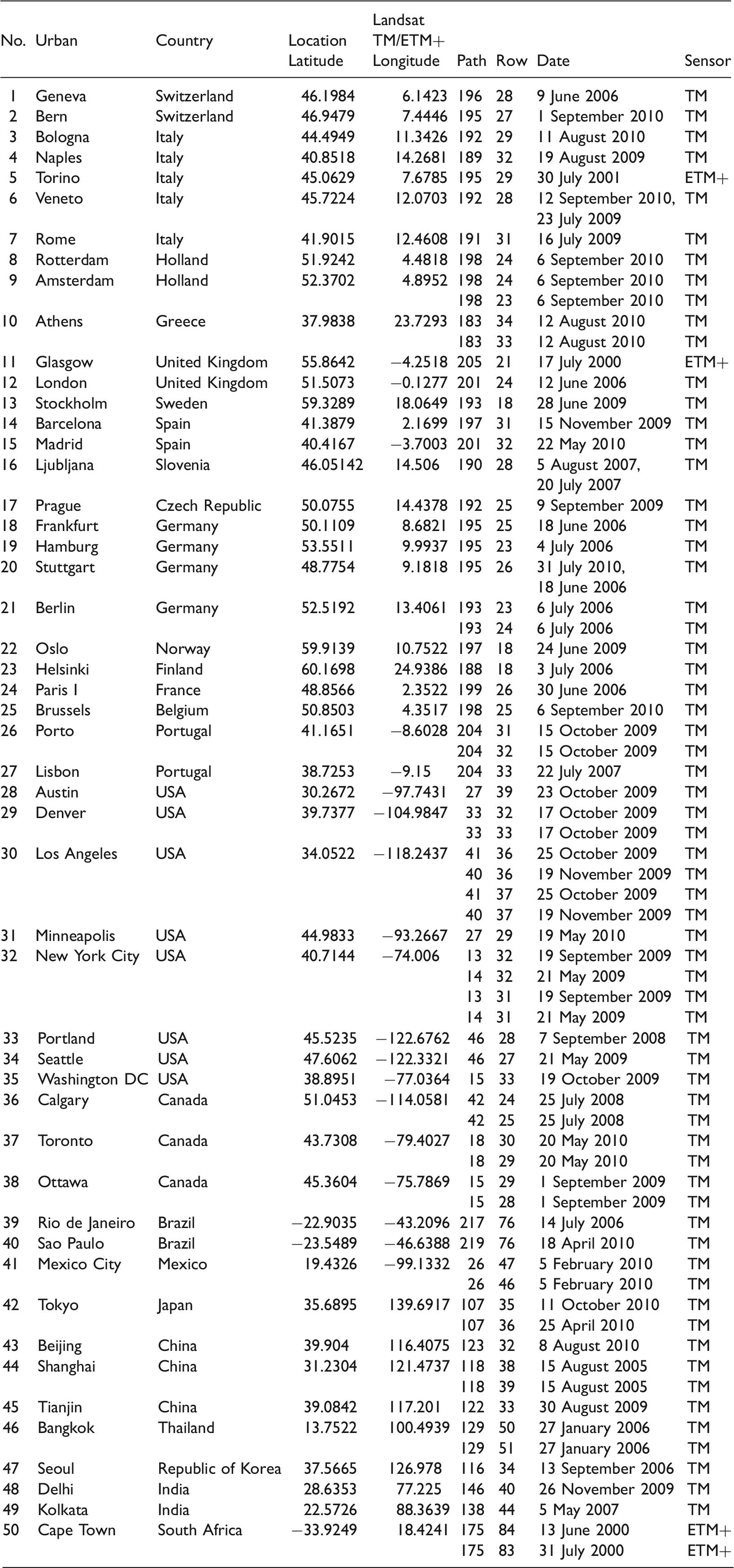
MODIS land cover type (MCD12Q1) products for 2005 with a spatial resolution of 500 m were obtained from the United States Geological Survey and used to delineate the urban boundaries of cities rather than using the administrative boundaries (Bagan and Yamagata, 2014). MCD12Q1 composites are publicly available at https://lpdaac.usgs.gov/products/modis (accessed 10 December 2016). The urban/built-up land cover class from the International Geosphere-Biosphere Programme land cover scheme of MCD12Q1 has been extracted (Bagan and Yamagata, 2014). The urban/built-up pixels were then buffered up to a distance of 10 km to define each urban boundary, except for Tokyo, for which we selected a nearly rectangular region to be consistent with previous studies (Letu et al., 2010).

Data

Landsat-derived land cover maps from around 2005 to 2010 (Table 1) and DMSP/OLS nighttime lights data were used in the study.

Although coarse spatial resolution (from 250 m to 2 km) monitoring provides global and national estimates of urban growth, coarse data might not be sufficiently reliable to accurately estimate the urban area of cities (Klotz et al., 2016; Lu et al., 2014; Potere and Schneider, 2007). Global availability of intercalibrated, accurately co-registered Landsat imagery with a 30 m resolution is ideal for extracting human settlements from different environments and cultures (Hansen and Loveland, 2012). Therefore, we selected Landsat-derived urban/built-up area data, which are independent from DMSP/OLS nighttime lights data, for the quantitative assessment of the mapping ability of DMSP/OLS nighttime lights for urban areas.

The land cover maps used in this study were derived from Landsat TM and ETM + images (Table 1; Bagan and Yamagata, 2014). The overall accuracy of the land cover maps for each city ranged from 77% to 95%. The land cover maps show six land cover classes, including built-up area. The built-up class includes all non-vegetative, human-constructed elements such as buildings, asphalt, concrete, and gravel. Other types of urban land use, such as golf courses, parks, and natural areas, are not included in the built-up class.

This study used version 4 of the DMSP/OLS stable lights product for 2005–2010 at a spatial resolution of 30 arc-seconds (1 km at the equator) (NGDC NOAA, 2013). The DMSP/OLS stable lights product archive was processed in annual increments by filtering the observations to remove the effects of moonlight, stray light, clouds, and ephemeral light sources such as fires and gas flares. Annual stable lights data are presented as DNs from 0 to 63, and DMSP/OLS nighttime lights composites are publicly available at www.ngdc.noaa.gov/eog/download.html (accessed 21 December 2016). For individual cities, we used DMSP/OLS stable lights data and Landsat TM/ETM + images from the same year to compare urban area results.

The population density of Tokyo in 2010 and the built-up area of Tokyo in 2009 were also used in additional quantitative analyses, which were considered useful because Japan provides accurate land use and population data gathered using a uniform and high-quality methodology. The population density was extracted from the Standard Grid Square population census data provided for every 5-year period from 1970 to 2015 by the Statistics Bureau, Japan (www.stat.go.jp/english/data/mesh/03.htm; accessed 10 December 2016). The Standard Grid Square (with a side of approximately 1 km) method divides all of Japan into meshes of approximately 1 km² based on latitude and longitude. The built-up land use area was extracted from the 2009 land use map with a spatial resolution of 100 m (http://nlftp.mlit.go.jp/ksj/gml/datalist/KsjTmplt-L03-b-u.html; accessed 11 December 2016). Built-up areas include seven categories: high-rise building, factory, low-rise building, low rise density building, road, railway, and public facility.

Methods

Grid-cell-based analysis

The advantage of using grid cells is that they enabled us to aggregate the categories for each map and to perform a quantitative analysis (Bagan and Yamagata, 2014; Im et al., 2016). We developed a DMSP/OLS nighttime lights pixel-derived grid cell approach, which facilitated a link between DMSP/OLS data and Landsat-derived built-up areas. Previous research developed an analytical method based on 1 km² grid cells to link DMSP/OLS nighttime lights data and land cover types (Bagan and Yamagata, 2015). This method involves overlaying the nighttime lights images onto a map with 1 km² grid cells, computing the percentage of the DN values of nighttime lights imagery within each cell, and storing the results in a new attribute table. The drawback of this method is that most of the attributes in the grid cells are zero, which may affect the efficiency of the statistical analysis. To avoid this limitation, our approach directly uses the DMSP/OLS nighttime light pixels to create the grid cells. The main steps of the proposed approach are as follows.

(a) We converted the DMSP/OLS nighttime light pixels to grid square cells for each city and assigned a unique ID to each grid cell. Thus, the resolution and geolocation of the grid cell are the same as the corresponding resolution and geolocation of the nighttime light pixel. Note that the grid cells for each city were generated individually to avoid a possible position gap in the DMSP/OLS nighttime light pixel locations of different years.

(b) We extracted the built-up area from the land cover maps of the 50 cities. We then overlaid the built-up area on the grid cells to compute the percentage of built-up area within each cell.

Because the proposed approach computes the percentage of built-up area within each nighttime light pixel, a spatially explicit evaluation of the relationship between the DMSP/OLS nighttime lights and urban area is feasible.

Quantitative analysis

To quantify the agreement between the built-up area estimated by the DMSP/OLS nighttime lights and the urban area derived from Landsat TM/ETM+, we (1) calculated the percentage of built-up area for each area corresponding to one pixel in the nighttime lights image and (2) tested the relationship between the percentage of built-up area and the DN value of the nighttime lights pixel for the 50 cities. The grid cells were sorted by percentage of built-up area in ascending order; calculation of the mean, median, and mode of the DMSP DN value was within intervals of 1% of built-up area (i.e. [0–1%], [1–2%], … [98–99%], [99–100%]). The correlation coefficients between the three statistical indicators (mean, median, and mode) of the DN value of the nighttime light pixel and the percentage of built-up area were then calculated.

The mean DN values were obtained by dividing the sum of the DN values of nighttime light pixels in the 1% interval (hereafter referred to as the “1% built-up interval”) by the number of nighttime light pixels within it. The median and mode were also estimated for each 1% built-up interval. The mean is given by

Mean = \frac{\sum_{i = 1}^{N} D N_{i}}{N}

(1)

where

D N_{i}

is the DN value of the ith nighttime light pixel and N is the total number of nighttime light pixels in a 1% built-up interval.

To calculate the median, we first arranged the sequence of DN values in ascending order. If the total number of nighttime light pixels was an odd number, the median is given by

Median = (\frac{N + 1}{2})^{th} term

(2)

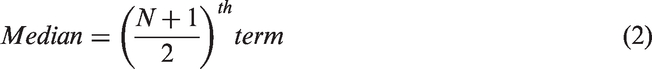
If the total number of nighttime light pixels was an even number, then the median is given by

M e d i a n = ({(\frac{N}{2})}^{t h} t e r m + {(\frac{N + 1}{2})}^{t h} t e r m) / 2

(3)

where N is the total number of nighttime light pixels in a 1% built-up interval.

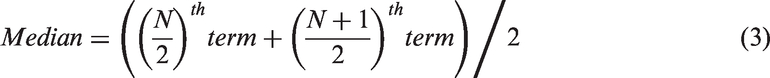
To calculate the mode, we first arranged the sequence of DN values in ascending order. If there were multiple values that occur equally frequently, we selected the smallest DN value as the mode.

Results

Analysis using Landsat-derived built-up area

Landsat-derived built-up area percentages of less than or equal to 20%, 30%, 50%, 70%, and 100% were exported separately, and the correlation coefficients between the percentage of built-up area in those regions and the corresponding DN value for nighttime light pixels were calculated (Figure 1).

Figure 1.

Correlation coefficient between the nighttime lights DN value and percentage of built-up area. The cities are listed in Table 1. The black, green, blue, magenta, and red lines correspond to the percentages of built-up area as noted in the legend.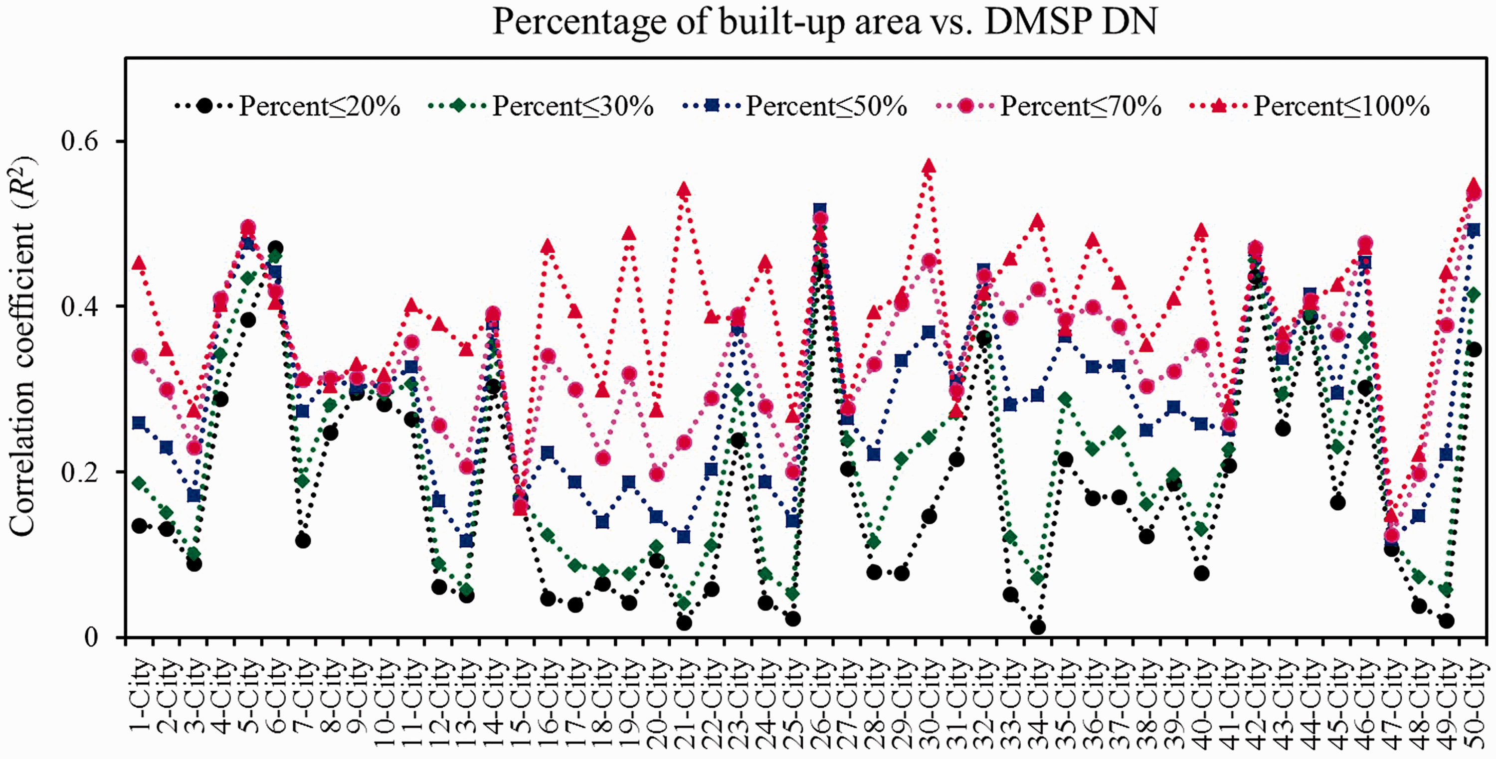

The correlation coefficients were generally higher as the percentage of built-up area increased, but the correlations were weak for most cities, even in low-density urban areas (built-up area ≤ 30%). Furthermore, there were almost no correlations in the low and moderate density urban areas (built-up area ≤ 70%) of Seoul, Delhi, Brussels, and Berlin (Table S1).

We also calculated the correlation coefficients between the percentage of built-up area for the various percentages and nighttime lights mean, median, and mode values (Figure 2). There is a relatively strong positive correlation between the nighttime lights mean and density of built-up area when the percentage of built-up area is ≤ 70%. However, the correlation between the percentage of built-up area and either the median or the mode of nighttime lights is weak for most of the cities.

Figure 2.

Correlation coefficient between the percentage of built-up area and the (a) mean, (b) median and (c) mode of the nighttime lights DN values. The cities are listed in Table 1. The black, green, blue, magenta, and red lines correspond to the percentages of built-up area as noted in the legend.

Comparison of the correlation coefficients between the percentage of built-up area and nighttime lights values (Figure 2) showed that the correlation coefficient between the percentage of built-up area and DMSP mean was relatively higher than that of the percentage of built-up area and DMSP median, or percentage of built-up area and DMSP mode in relatively low-density urban areas (built-up area ≤ 50%). In contrast, the correlation coefficient between the percentage of built-up area and DMSP median, or percentage of built-up area and DMSP mode were weak in most of the cities (Table S2).

We also examined the relationship of the spatial distribution of the DN of nighttime lights imagery and the density of built-up areas. Figure 3 shows scatter plots of the relationship for all of the grid cells in Los Angeles, Bangkok, Shanghai, Barcelona, Beijing, Athens, Delhi, and Seoul. Due to space constraints, we display only these eight cities rather than all of the 50 cities.

Figure 3.

Scatter plots illustrating the relationship between the percentage of built-up area from Landsat imagery vs. the nighttime lights DN values at the grid cell scale in Los Angeles, Bangkok, Shanghai, Barcelona, Beijing, Athens, Delhi, and Seoul.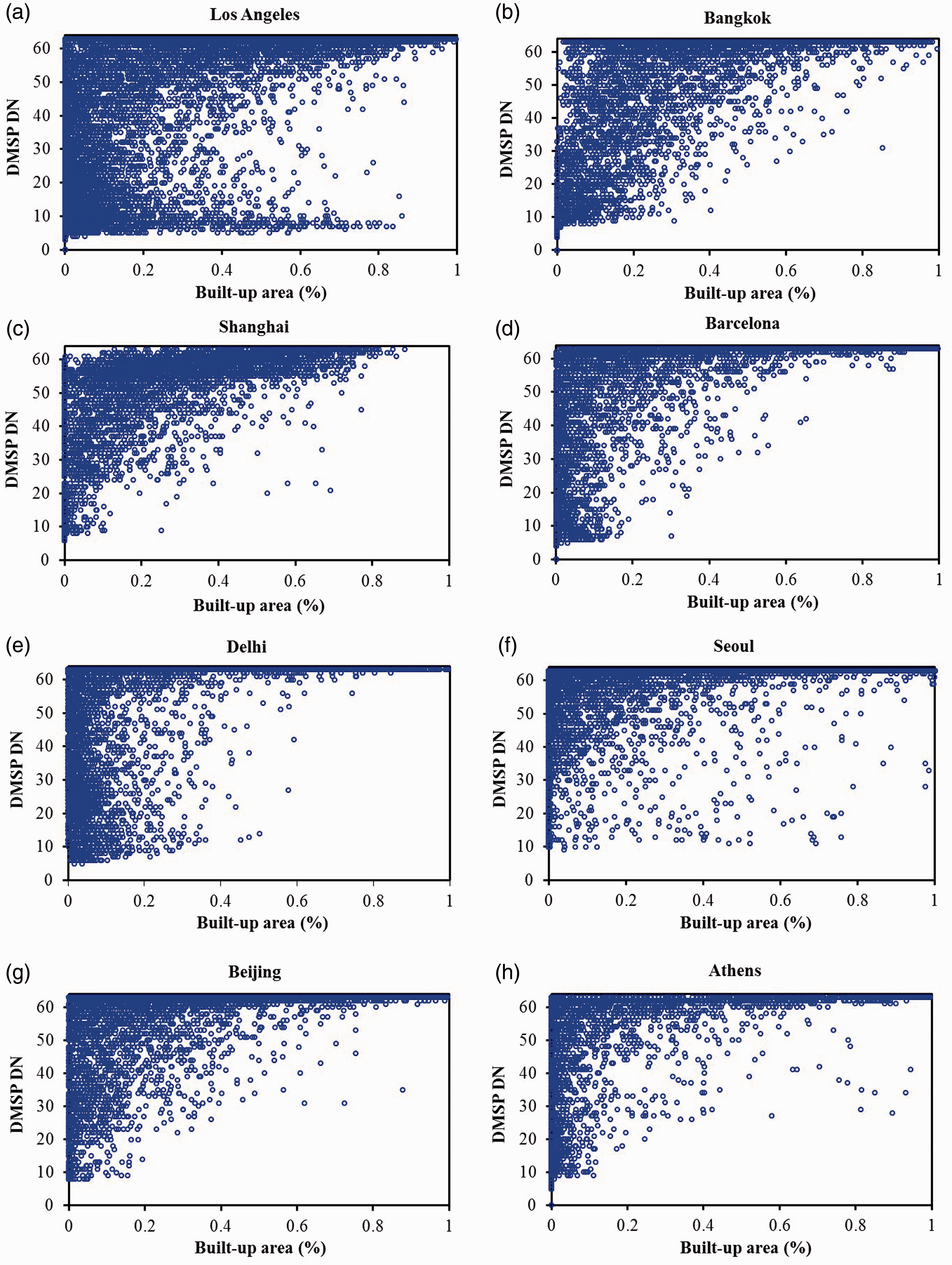

Although positive correlations are evident in low-density built-up areas, the correlations are low for each of these cities. Additionally, the relationships are extremely noisy. Therefore, the nighttime lights DN values do not seem to be sensitive to variations in built-up area density, and none of the correlations is statistically significant (p-value < 0.0001). Contrary to the assumption that most of the high nighttime lights DN value pixels will be distributed in the city cores, a large number of high nighttime lights DN value pixels were also distributed in low-density built-up areas (Figure 3). As a result, the correlation coefficients are low even in regions where the percentage of built-up area is ≤30%; in fact, the R² values between the brightness of nighttime lights and a built-up area density of ≤30% were 0.24 (Los Angeles), 0.36 (Bangkok), 0.39 (Shanghai), 0.35 (Barcelona), 0.29 (Beijing), 0.29 (Athens), 0.07 (Delhi), and 0.12 (Seoul) (Figure 1).

To visualize the weak correlation more clearly, we selected the land cover maps of Beijing and Athens to highlight the relationship between brightness of nighttime lights and percentage of built-up area. As Figure 4 shows, the area indicated by high nighttime lights DN value pixels is larger than the built-up area in both cities (compare panels (a) to (d) in Figure 4). We also extracted the nighttime lights DN values that were >49 and cells with a built-up area density of ≤20% and then overlaid the extracted grid cells (rectangle polygons) onto the built-up area percentage maps (Figure 4(e) and (f)).

Figure 4.

Land cover (a, b), DMSP/OLS nighttime lights DN value (c, d), and built-up area percentage maps with extracted grid cells (e, f) in Beijing and Athens.

The spatial distribution of built-up area density is considerably different from the shape of the nighttime lights DN value magnitude map. For example, it is clear that high nighttime lights DN values are distributed in low-density areas. Furthermore, the spatial distributions of higher DN value pixels in low-density areas are generally not related to land cover type.

Because the high nighttime lights DN value pixels are distributed throughout low-density built-up areas, it is difficult to use the built-up areas to detect the optical threshold for mapping urban areas from nighttime lights. It is also difficult to use low-density built-up areas to build a regression model to calibrate saturated nighttime light pixels.

Relationships between nighttime lights, land use map, and population census data in Tokyo

As an alternative to using built-up area derived from land cover mapping, we used the built-up area derived from a 2009 land use map to examine the relationship between built-up area and brightness of nighttime lights for Tokyo. We also examined the relationship between population density and brightness of nighttime lights for Tokyo.

The spatial distributions of the two types of built-up area maps differ considerably from the nighttime lights imagery (Figure 5(a) to (c)). The area of high DN value pixels is far larger than either of the two types of built-up area. In contrast, the spatial distribution of the population density (Figure 5(d)) is highly consistent with the two types of built-up area maps.

Figure 5.

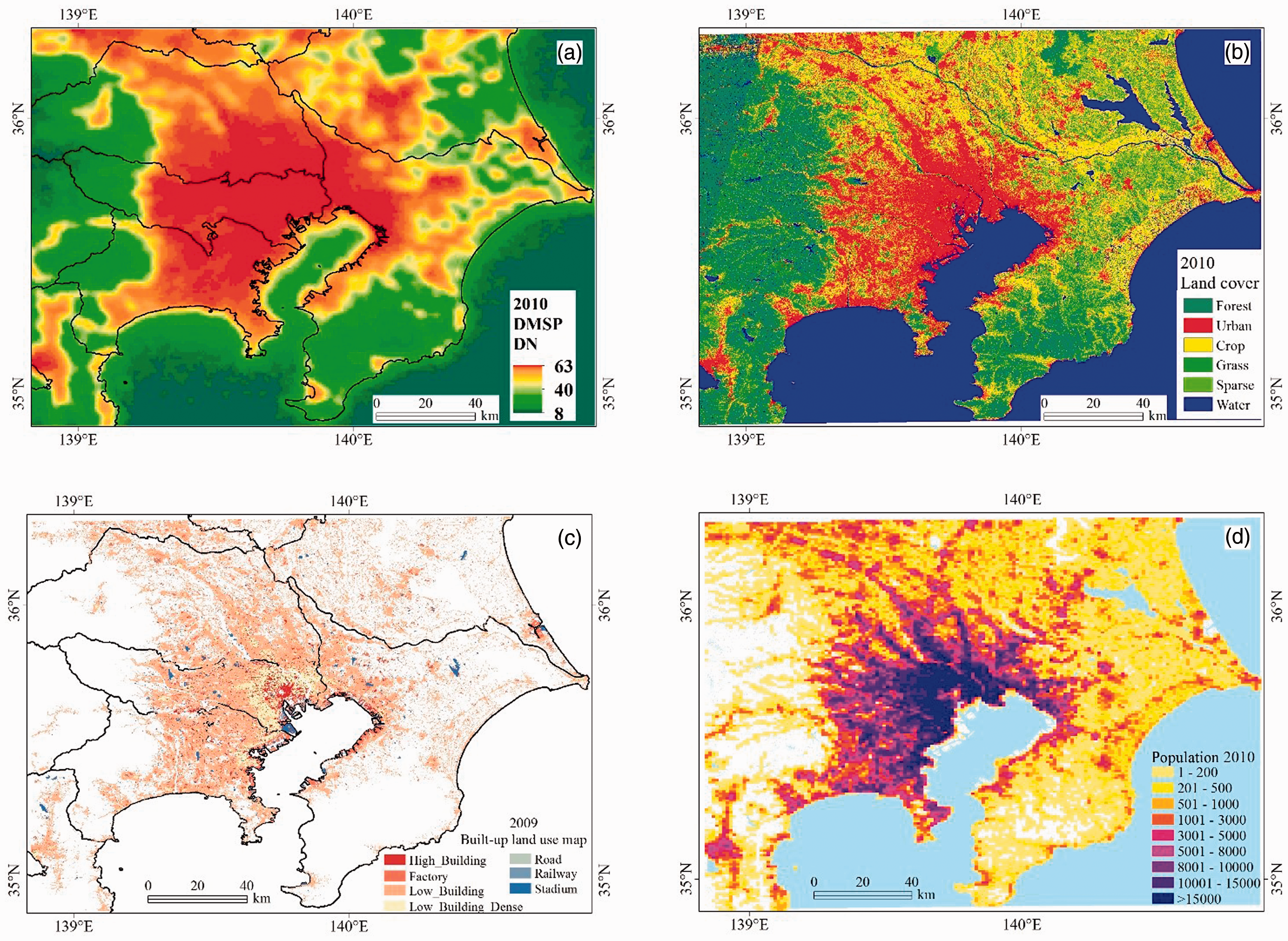
We aggregated the seven built-up categories in the built-up land use map of 2009 into one category to facilitate the comparison. We then overlaid the aggregated built-up land use map of 2009 onto the grid square cells derived from nighttime lights to compute the percentage of built-up land use area within each cell (Figure 6).

Figure 6.

Scatter plots for Tokyo of (a) density of built-up area derived from land cover vs. density of built-up area derived from the land use map; (b) density of built-up area derived from land cover vs. nighttime lights; and (c) density of built-up area derived from the land use map vs. nighttime lights.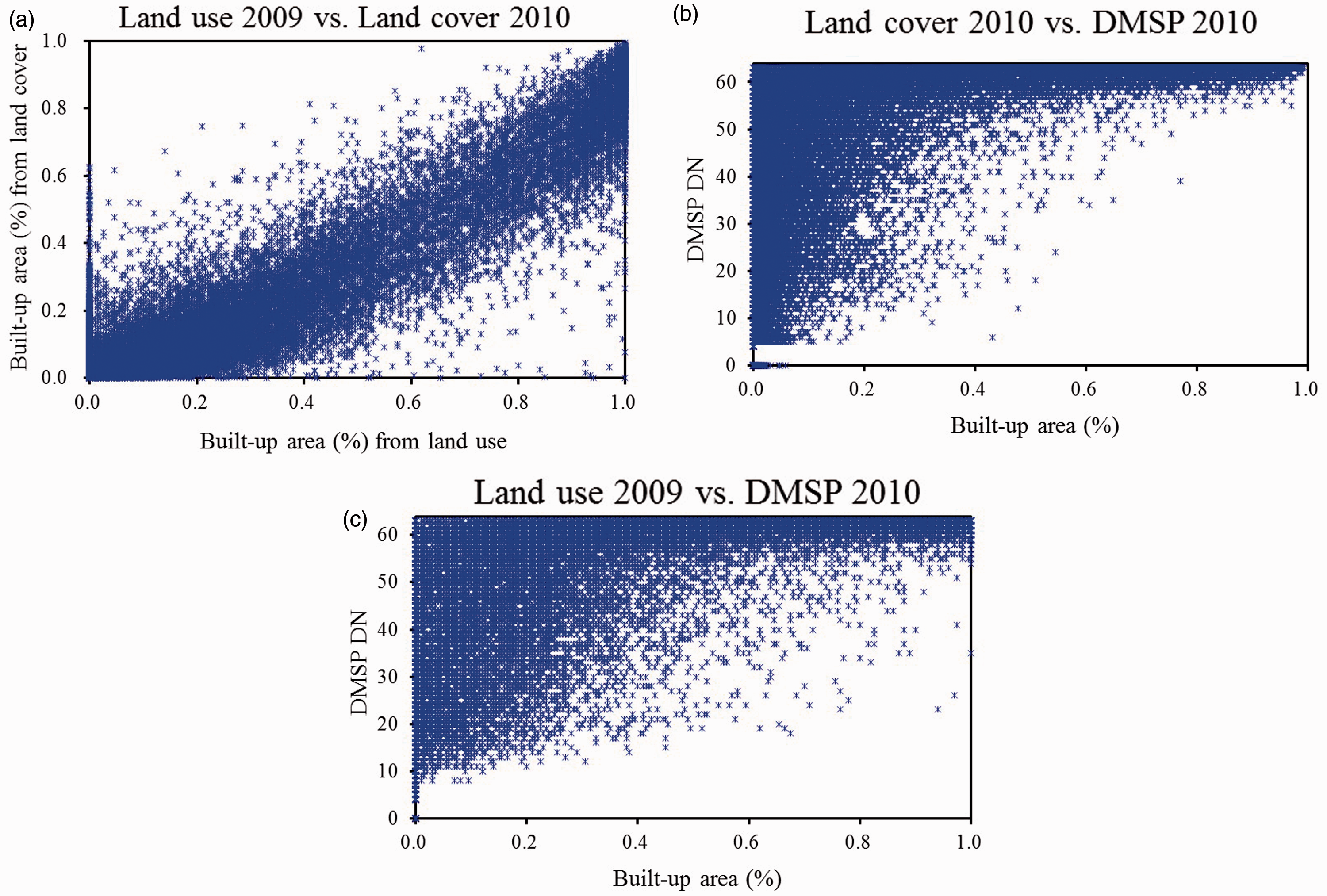

As Figures 5 and 6 illustrate, there was little difference between the built-up area density maps derived from land cover and land use. The spatial distributions of built-up area derived from land cover and land use are highly consistent with each other and have a high positive correlation coefficient (R² = 0.90, p-value < 0.0001). In contrast, both built-up area density maps have weak correlations with nighttime lights (R² = 0.47 and R² = 0.53, respectively, p-value < 0.0001).

As before (Figure 4(e) and (f)), we extracted the grid cells (regions) that had high brightness values (nighttime lights DN > 49) and low built-up density (≤20%) from the land cover map for Tokyo, but we also used the land use map. We then overlaid the extracted grid cells onto the built-up area maps derived from land cover and land use (Figure 7).

Figure 7.

Spatial distribution of high DN values of nighttime light pixels in low-density built-up areas in Tokyo: (a) nighttime lights vs. built-up area derived from land cover; (b) nighttime lights vs. built-up area derived from land use.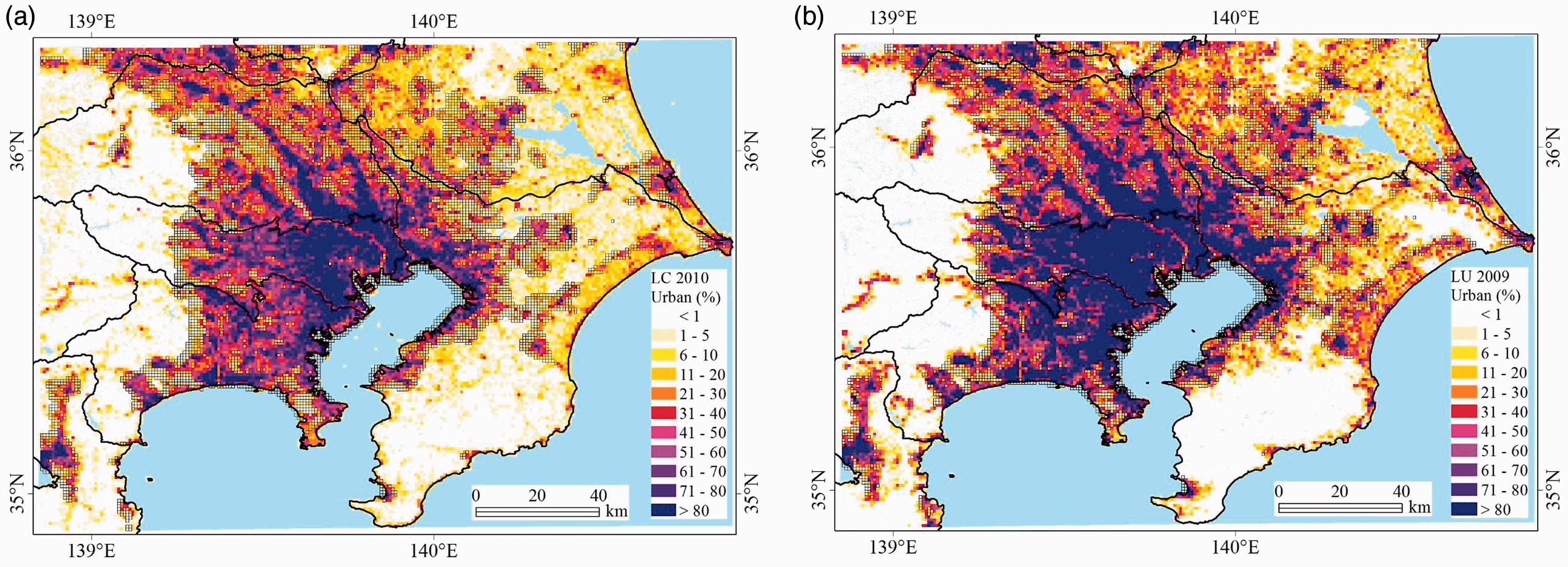

As Figure 7 shows, many of these bright nighttime light pixels were haphazardly distributed in low-density areas on the built-up area maps derived from both land cover and land use. Hence, the DMSP/OLS nighttime light brightness values do not appear to be sensitive to built-up density variations in Tokyo.

We also overlaid the nighttime light pixels that have a high DN value (>49) on the population density map of 2010 (Figure 8). As Figure 8 shows, in the center part of Tokyo, despite the population density being low, nighttime lights DN values generally exceed 49. However, in the other sparsely populated regions of Tokyo, there are almost no nighttime lights DN values that exceed 49, despite the population density being greater than 500 person/km². As Figure 8 shows, the largest discrepancies occur mostly in suburban and rural areas. This indicates that the brightness of nighttime lights is strongly affected by the surrounding environment, regardless of population.

Figure 8.

Spatial distribution of high DN values of nighttime light pixels on the population density map of 2010.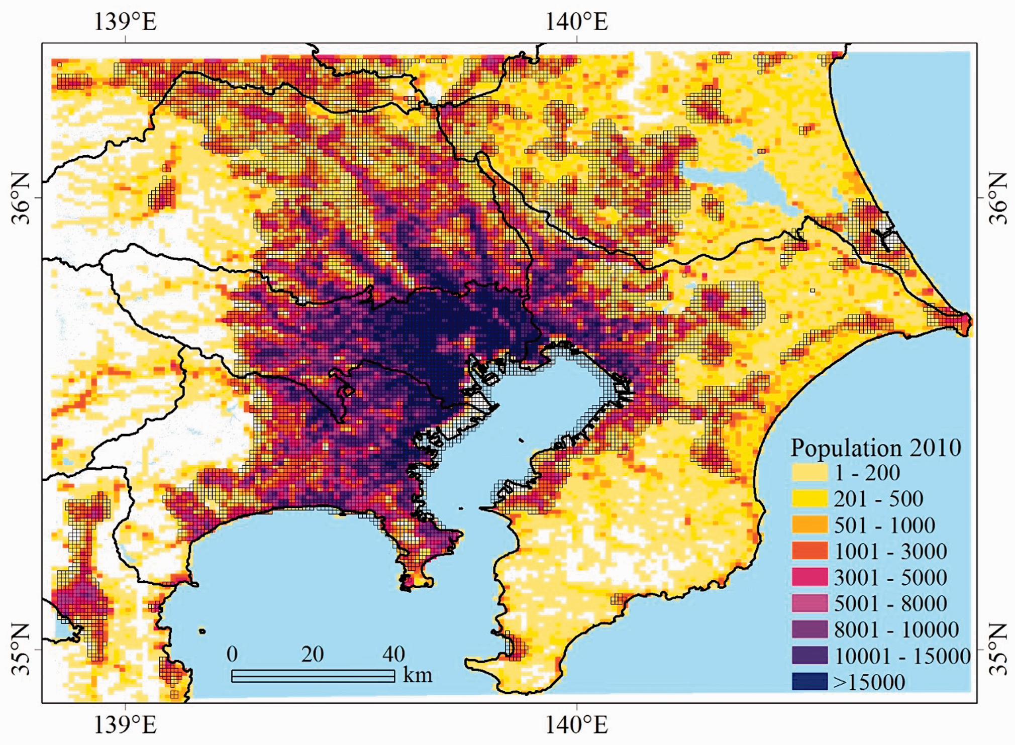

Discussion

Although previous studies have evaluated the utility of DMSP/OLS nighttime light data for mapping regionally and globally consistent urban areas, e.g., by using optimal thresholds methods (Henderson et al., 2003; Wei et al., 2014) or by using low-density urban built-up areas to calibrate saturated nighttime light pixels via regression models (Letu et al., 2010), our study reveals that nighttime lights imagery itself is not an effective tool to delimit urban extents. As shown in Figures 3 and 4, many bright nighttime light pixels (DN > 49) are haphazardly distributed in low-density built-up areas (built-up rate ≤ 20%). On the other hand, as Figures 7 and 8 show, the DN values of nighttime light pixels were mostly less than 50 in the western and southeastern parts of Tokyo, even though the built-up area density was greater than 30% and the population density was greater than 1000 person/km². Therefore, nighttime light data tend to overestimate the built-up area in large cities but may tend to reduce the built-up area in less populated areas.

Landsat daytime imagery can discriminate between various types of land use/land cover because of the various spectral bands, whereas OLS nighttime imagery only provides single-channel observations and primarily measures light from outdoor infrastructure. Henderson et al. (2003) noted that non-urban land cover types in Landsat classification maps such as the lit pathways of parks and peri-urban areas contribute to a city's light emissions, which partly cause the brightness of nighttime lights to be weakly correlated with built-up rate.

Moreover, many bright nighttime light pixels (DN > 49) are haphazardly distributed in low-density built-up areas; thus, it is difficult to use them to determine the nighttime lights in optimal threshold methods for mapping urban areas. Furthermore, since small cities and towns are almost always excluded from high DN value nighttime light regions, it may be difficult to reduce the effect of nighttime light saturation effectively and to increase the variation of nighttime light signals by using a regression function or vegetation-index-based methods.

Therefore, irrespective of the desired function, limitations exist when using only DMSP/OLS stable light image products to map urban areas.

Conclusions

Our results provide an overview of the relationship between nighttime lights and density of built-up areas for 50 cities across the globe. Linking DMSP/OLS nighttime lights with built-up density via grid cells is an attractive approach for quantifying the capacity of DMSP/OLS nighttime light data to map regional and global urban areas. DMSP/OLS-derived grid cells have previously exhibited great potential for estimating spatially explicit urban variables over a range of geographic scales.

The results of this work indicate that there are no significant correlations between DMSP/OLS nighttime lights and density of built-up areas (p-value < 0.0001). This study also provides insights for future work to improve the accuracy of the DMSP/OLS-based urban area estimations. Regarding future activities, it is important to use the Landsat-based Global Human Settlement Layer (Pesaresi et al., 2016) or the new Global Urban Footprint (Esch et al., 2017) dataset derived from SAR imagery to assess the capacity of DMSP/OLS for urban area mapping.

Footnotes

Acknowledgements

This research was supported by the Environment Research and Technology Development Fund (S-10) of the Ministry of the Environment, Japan and supported by the NSFC (Grant No. 41771372).

Declaration of conflicting interests

The author(s) declared no potential conflicts of interest with respect to the research, authorship, and/or publication of this article.

Funding

The author(s) received no financial support for the research, authorship, and/or publication of this article.

Supplemental material

Supplemental material is available for this article online.

Hasi Bagan received the B.S. degree in mathematics from the Peking University, China, in 1991, the M.S. degree from the Beijing University of Aeronautics and Astronautics, China, in 1996, and the Ph.D. degree from the Institute of remote sensing applications, Chinese Academy of Sciences, China, in 2004. From 2004 to 2016, he was a research associate with the National Institute for Environmental Studies, the University of Tokyo, and the Ibaraki University, Japan. He is currently a Professor at the Institute of Urban Studies, Shanghai Normal University, China. His research interests are urban growth analysis, neural network, wavelet fusion, and subspace algorithms.

Habura Borjigin received the B.S. and M.S. degree from the Inner Mongolia Normal University, China, in 2002 and 2006, and the Ph.D. degree from the Graduate School of Geo-Environmental Science, Rissho University, Japan, in 2012. He is currently a research associate with the National Institute for Environmental Studies, Japan. His research interests are land cover classification and urban growth analysis.

Yoshiki Yamagata graduated from the University of Tokyo (PhD in System Science). Since 1991, he works at the National Institute for Environmental Studies. Currently, he is studying about the climate risk management as Principal Researcher of Center for Global Environmental Research (CGER). He is also affiliated with IIASA (Vienna) and Institute of Statistical Mathematics (ISM, Tokyo). His recent research topics include: Land use scenarios, resilient urban planning and spatial network analysis. He has lecture series at the University of Tokyo, University of Tsukuba and Hokkaido University. Internationally, he has contributed as Lead Author of IPCC, Steering Committee of “Global Carbon Project”.

References

Bagan

Yamagata

(2014) Land-cover change analysis in 50 global cities by using a combination of Landsat data and analysis of grid cells. Environmental Research Letters 9(6): 064015.

Bagan

Yamagata

(2015) Analysis of urban growth and estimating population density using satellite images of nighttime lights and land-use and population data. GIScience & Remote Sensing 52(6): 765–780.

Baugh

Elvidge

Ghosh

et al. (2010) Development of a 2009 stable lights product using DMSPOLS data. Proceedings of the Asia-Pacific Advanced Network 30: 114–130.

Chen

Nordhaus

(2011) Using luminosity data as a proxy for economic statistics. Proceedings of the National Academy of Sciences of the United States of America 108: 8589–8594.

Doll

(2008) CIESIN Thematic Guide to Night-Time Light Remote Sensing and its Applications, Palisades, NY: Center for International Earth Science Information Network of Columbia University.

Elvidge

Baugh

Kihn

et al. (1997) Relation between satellite observed visible-near infrared emissions, population, economic activity and electric power consumption. International Journal of Remote Sensing 18: 1373–1379.

Elvidge

Baugh

Zhizhin

et al. (2017) VIIRS night-time lights. International Journal of Remote Sensing 38(21): 5860–5879.

Elvidge

Baugh

Zhizhin

et al. (2013) Why VIIRS data are superior to DMSP for mapping nighttime lights. Proceedings of the Asia-Pacific Advanced Network 35: 62–69.

Elvidge

Cinzano

Pettit

et al. (2007a) The Nightsat mission concept. International Journal of Remote Sensing 28(12): 2645−2670.

10.

Elvidge

Tuttle

Sutton

et al. (2007b) Global distribution and density of constructed impervious surfaces. Sensors 7: 1962–1979.

11.

Esch

Heldens

Hirner

et al. (2017) Breaking new ground in mapping human settlements from space – The Global Urban Footprint. ISPRS Journal of Photogrammetry and Remote Sensing 134: 30–42.

12.

Fragkias M, Lobo J and Seto KC (2016) A comparison of nighttime lights data for urban energy research: Insights from scaling analysis in the US system of cities. Environment and Planning B 44(6): 1077–1096.

13.

Hansen

Loveland

(2012) A review of large area monitoring of land cover change using Landsat data. Remote Sensing of Environment 122: 66–74.

14.

Liu

Tian

et al. (2014) Urban expansion dynamics and natural habitat loss in China: A multiscale landscape perspective. Global Change Biology 20(9): 2886–2902.

15.

Henderson

Yeh

Gong et al. (2003) Validation of urban boundaries derived from global night-time satellite imagery. International Journal of Remote Sensing 24: 595–610.

16.

Park

Rhee

et al. (2016) Downscaling of AMSR-E soil moisture with MODIS products using machine learning approaches. Environmental Earth Sciences 75: 1120.

17.

Imhoff

Lawrence

Stutzer

et al. (1997) A technique for using composite DMSP/OLS “city lights” satellite data to map urban areas. Remote Sensing of Environment 61: 361−370.

18.

Klotz

Kemper

Geiß

et al. (2016) How good is the map? A multi-scale cross-comparison framework for global settlement layers: Evidence from Central Europe. Remote Sensing of Environment 178: 191–212.

19.

Letu

Hara

Yagi

et al. (2010) Estimating energy consumption from night-time DMPS/OLS imagery after correcting for saturation effects. International Journal of Remote Sensing 31: 4443–4458.

20.

Levin

Phinn

(2016) Illuminating the capabilities of Landsat 8 for mapping night lights. Remote Sensing of Environment 182: 27–38.

21.

Liu

Delahunty

Zhao

et al. (2016) These lit areas are undeveloped: Delimiting China's urban extents from thresholded nighttime light imagery. International Journal of Applied Earth Observation and Geoinformation 50: 39–50.

22.

Rhee

et al. (2014) Building type classification using spatial and landscape attributes derived from LiDAR remote sensing data. Landscape and Urban Planning 130: 134–148.

23.

Miller

Mills

Elvidge

et al. (2012) Suomi satellite brings to light a unique frontier of nighttime environmental sensing capabilities. Proceedings of the National Academy of Sciences 109: 15706–15711.

24.

NGDC NOAA National Geophysical Data Center (2013) Version 4 DMSP-OLS nighttime lights time series. Available at: www.ngdc.noaa.gov/eog/dmsp/downloadV4composites.html (accessed 10 November 2017).

25.

Oda

Maksyutov

(2011) A very high-resolution (1 km × 1 km) global fossil fuel CO₂ emission inventory derived using a point source database and satellite observations of nighttime lights. Atmospheric Chemistry and Physics 11: 543–556.

26.

Pesaresi M, Ehrlich D, Ferri S, et al. (2016) Operating Procedure for the Production of the Global Human Settlement Layer from Landsat Data of the Epochs 1975, 1990, 2000, and 2014. JRC Technical Report EUR 27741 EN; doi:10.2788/253582 (online).

27.

Potere

Schneider

(2007) A critical look at representations of urban areas in global maps. GeoJournal 69(1): 55–80.

28.

Stathakis D (2015) Deriving soil sealing degree from nighttime VIIRS imagery. In: IGARSS 2015.

29.

Stathakis

Tselios

Faraslis

(2015) Urbanization in European regions based on night lights. Remote Sensing Applications: Society and Environment 2: 26–34.

30.

Sutton

(2003) A scale-adjusted measure of “Urban sprawl” using nighttime satellite imagery. Remote Sensing of Environment 86: 353–369.

31.

Tan

(2017) An intensity gradient/vegetation fractional coverage approach to mapping urban areas from DMSP/OLS nighttime light data. IEEE Journal of Selected Topics in Applied Earth Observations and Remote Sensing 10(1): 95–103.

32.

Wei

Liu

Song

et al. (2014) Normalization of time series DMSP-OLS nighttime light images for urban growth analysis with pseudo invariant features. Landscape and Urban Planning 128: 1–13.

33.

Peng

et al. (2013) Intercalibration of DMSP-OLS nighttime light data by the invariant region method. International Journal of Remote Sensing 34: 7356–7368.

34.

Xie

Weng

(2016) Updating urban extents with nighttime light imagery by using an object-based thresholding method. Remote Sensing of Environment 187(15): 1–13.

35.

Zhang

Pandey

Seto

(2016) A robust method to generate a consistent time series from DMSP/OLS nighttime light data. IEEE Transactions on Geoscience and Remote Sensing 54: 5821–5831.

36.

Zhang

Schaaf

Seto

(2013) The vegetation adjusted NTL urban index: A new approach to reduce saturation and increase variation in nighttime luminosity. Remote Sensing of Environment 129: 32–41.

37.

Zhao

Liu

Cao

et al. (2017) Forecasting China's GDP at the pixel level using nighttime lights time series and population images. GIScience & Remote Sensing 54(3): 407–425.

38.

Zhou

Smith

Elvidge

et al. (2014) A cluster-based method to map urban area from DMSP/OLS nightlights. Remote Sensing of Environment 147: 173–185.

39.

Zhuo

Zheng

Zhang

et al. (2015) An improved method of night-time light saturation reduction based on EVI. International Journal of Remote Sensing 36: 4114–4130.

Supplementary Material

Please find the following supplemental material available below.

For Open Access articles published under a Creative Commons License, all supplemental material carries the same license as the article it is associated with.

For non-Open Access articles published, all supplemental material carries a non-exclusive license, and permission requests for re-use of supplemental material or any part of supplemental material shall be sent directly to the copyright owner as specified in the copyright notice associated with the article.

0.00 MB

0.36 MB