Urban scaling and the geographic concentration of inequalities by city size

Abstract

Urban scaling laws summarise how socio-economic behaviours of urban systems may be predicted from city size. While most scaling analysis rests on using aggregate quantities (total incomes, GDP, etc.), examining distributions of these aggregate quantities (e.g. income distributions) could shed light on how socio-economic inequalities may correlate or be causally linked to city size. In this direction, this paper examines how geographic distributions and spatial inequalities of income and housing costs vary by city size. The paper presents three principal results. First, it brings out qualitative implications of quantitative scaling by relating scaling of the distributions of income and housing costs to their specific geographic concentrations. Second, it shows that some small and medium sized cities are clear outliers, showing behaviour similar to the largest cities and starkly different from the behaviours of the bulk of small and medium sized cities. Third, this above observation explains why heteroscedasticity, or large and heterogeneous fluctuations, are frequently observed in urban indicator data when plotted as a function of city size. Putting together these three results, overall, it is shown that income distributions and housing costs scale and concentrate in cities by size in a predictable way, where the largest cities superlinearly/disproportionately agglomerate the highest income earners and the highest housing costs, and show relatively lower concentrations of low-middle income earners and low-medium housing costs. In contrast, most of the smaller and medium sized cities show a ‘flipped’ opposite trend. A few small and medium sized cities are outliers: they show trends that match those of the largest cities, due to specialisations of economic functions or concentrations of high-paying occupations in these cities. The empirical findings lead to a discussion on the objective and normative relationships between city size and urban inequalities. It is suggested that due to the concentrations of high income and high housing costs, largest cities may have a resulting housing market structure that will push out lower and medium income earners, thereby making affordability, diversity, and socio-spatial justice emerge as important urban policy issues.

Keywords

Agglomeration and city size inequality income distributions housing cost distributions spatial concentration scaling laws fluctuations Australia USA

Introduction

The earliest economic arguments for why cities exist were provided by theories of agglomeration: human productivity, consumption and exchange occur through organised systems of interactions, and the costs of such interaction are reduced by locating them close together in space (Marshall, 1920). Modern day urban economics and geography theorises on several factors to account for agglomeration, such as natural advantages of certain geographic locations, reductions in transaction and transportation costs in producing, transporting and consuming goods, knowledge spillovers and positive externalities from technology and skills, and the propensity for innovations, diversification and specialisations to emerge (Fujita, 1989; Fujita and Thisse, 2013; Glaeser and Resseger, 2010; Pumain, 2004, 2006).

How the size of an urban system, measured via total population, densities, or spatial spread, relates to socio-economic growth processes is thus a fundamental topic for urban science. An empirical approach that captures the regularities of how socio-economic quantities grow with city size employs urban allometric scaling laws (Batty, 2013; Bettencourt et al., 2007; Pumain, 2004, 2006). This line of research has recently been resuscitated (Bettencourt et al., 2007), even though references to allometric scaling models are seen as far back as the 1950s (Beckmann, 1958) and the modern resurgence of these ideas have been formulated via urban complex systems approaches (Pumain, 2004, 2006). The idea is captured through a simple model, echoing Marshallian principles of agglomeration: $Y = α X^{β}$ , where Y is a socio-economic quantity or indicator, X is measure of city size, usually its population, α is a proportionality constant, and β is the scaling exponent on which the behaviour of the system rests. If $β = 1$ , growth in Y is linear/proportional with growth in X. If $β < 1$ (sub-linear), growth in Y is less than proportional (economies of scale), if $β > 1$ (superlinear), growth in Y is higher than proportional with growth in X (increasing returns to scale).

A lot of research focuses around the increasing returns to scale idea on how productivity, industrial diversity or wealth scales with city size. The growth of an urban system occurs as a natural consequence of the fundamental tendencies of human beings to work together to produce, consume and exchange. Thus, through a classic preferential attachment argument, growth leads to more growth. The larger a city, the more likely that it will sustain the kind of diversity or specialisations developing for even more diversity or specialisation to develop, and thus has a larger likelihood of attracting more people. Bettencourt et al. (2007) empirically demonstrated that larger cities are both more productive and efficient, producing superlinear growth of economic outputs (e.g. total wages, income, number of patents, or GDP) for sub-linear growth rates of inputs (e.g. numbers of gas stations, lengths of infrastructure networks). Further, it has been proposed that larger cities provide more opportunities for more individual specialisation co-existing with overall increases in diversification (Bettencourt et al., 2015). Such diversification may be differentially dependent on the evolutionary innovation stage at which an industry or technology phase sits (Pumain et al., 2006). In addition, there are knowledge and skills premiums, connecting urban size, density and productivity. Glaeser and Resseger (2010) find as evidence for the existence of agglomeration economies: higher urban density and bigger cities attract not simply more workers, but more skilled workers. Moreover, urban systems could have a critical mass or threshold size, below which higher order industries or diversification may not exist (Mori et al., 2008).

Nonetheless, many of these findings are still open to debate, since empirical research rests on specific definitions of spatial units for analysis as well as industry sectoral classifications. Altering the definitions of the spatial units that were defined as ‘cities’ or ‘urban aggregates’ could alter the estimation of the value of the scaling exponents (Arcaute et al., 2015; Louf and Barthelemy, 2014). The scaling exponent for the same urban indicator was estimated to be superlinear with some geographic definitions, but sub-linear or linear with others. In a similar vein of examining such ecological fallacy or modifiable area unit problems, Mameli et al. (2008) examined alternate definitions of industry sectors keeping the geographic/spatial units constant. They too found that the models were highly sensitive to varying definitions of sectoral aggregation or classification.

With increasing returns to scale, the diseconomies produced by density and scale: congestion, travel times, pollution and crime, also rise. As cities grow larger and denser, it takes longer to do the journey to work commute or travel to other activities. Since more and more people share these aims, there are increases in congestion. Intra-city spatial sorting occurs as differentials and gradients of land-use generated values within a city cause residents to organise in locations that face trade-offs between rents and travel costs. Inter-city spatial sorting occurs as differentials and gradients of opportunities and returns between cities cause residents to prefer cities that promise higher returns while maximising quality of life. In economic geography, this is characterised as the tension between centripetal forces, that concentrate economic activity, and centrifugal forces, that oppose such concentration (Fujita et al., 1999). Empirical research shows the rise of what is termed the consumer city: urban structures in which highly skilled workers choose to pay high costs to live in dense neighbourhoods that provide high levels of service and consumption opportunities (Florida, 2004; Glaeser et al., 2001). The policy implications of such findings for spatial and social justice are, however, less clear.

This paper focuses on two aspects that warrant further attention in urban scaling research:

The role of distributions

Scaling laws in their current form usually measure the performance of a city through its aggregative characteristics, quantities or indicators (e.g., total incomes, GDPs, or numbers of patents) between cities. While questions of aggregation are fundamental and important in measuring city performance, questions of distribution are equally important and warrant further attention. Examples of distribution are income, rent, mortgage, travel costs, or accessibility distributions within and between cities. If a city produces superlinear growth of economic returns to sub-linear growth of inputs, it is likely that policy outcomes would lean towards incentivising growth in aggregative terms: larger cities being preferred over smaller or medium sized ones.

But, how is this higher economic return being distributed? Previous research done on industrial sectors has found that different parts of a distribution may fall in different scaling regimes, even when the overall aggregate behaviour falls in one particular regime: linear, sub-linear, or superlinear (Pumain et al., 2006). Thus, in studying scaling, it is as essential to study distributions of an urban indicator as it is to study its overall aggregative behaviour.

The distribution question is specifically important for income and housing/living costs. If larger cities produce more economic outputs, how is this output distributed or how does it affect social equity, overall productivity and spatial justice, both demographically as well as spatially? The final aim of producing economic output is to increase the well-being of the human condition: economic production and technological innovation are not ends in themselves, no matter how efficiently produced by any system of organisation (a large or “smart” city in this case), they are the means (and only a partial one) by which well-being and higher productivity is achieved. Thus, it is an important aim to unpack and understand how the growth of cities and agglomeration affects aspects of distribution, and therefore by extension, well-being or overall productivity. Recent research has shown that larger cities could be more unequal in their distributive aspects (Behrens and Robert-Nicoud, 2013; Cottineau et al., 2016; Pavan and Baum-Snow, 2013; Sarkar et al., 2016) and that these effects could range from intercity to intracity scales (Bradbury, 2017).

The role of fluctuations

Previous research also demonstrates that data on urban indicators shows heteroscedasticity: the urban indicator Y shows large and heterogeneous fluctuations as a function of the population size X (Leitao et al., 2016), making it hard to claim with certainty the type of statistical model that could be generating the data. In qualitative terms, this implies that while a general scaling trend is observed, frequent outliers or large deviations may also be observed simultaneously. Cities of the same size can show large deviations over the urban indicator measured. On the other hand, cities of different sizes could be performing at similar levels on the particular urban indicator being measured. This is particularly evident for smaller and medium sized cities, of which there are many more, as compared to larger sized cities. Thus, it is essential to study these fluctuations as well as their qualitative implications for urban systems. Previous research (Pumain, 2006, 2012) points out the currently open question of why an urban hierarchy (the organisation of cities into heterogeneous size distributions) emerges. The alternative explanation to scaling is proposed: a hierarchical manner in which innovations at different stages of development diffuse through the urban system, with older and more mature technologies growing sub-linearly, middle-stage technologies growing linearly and new technologies growing superlinearly with city size. What is not yet sufficiently explored are questions of consumption: how do these types of hierarchical differentiations of production affect the organisation of consumption, and the questions of resulting socio-spatial justice, losses of overall productivity, and spatial inequalities that arise in income distributions and costs of living.

This, it is essential to explore scaling behaviours in the light of urban hierarchies: do smaller and medium sized cities behave in a fundamentally different way than the largest cities? In this paper, there is a particular focus on (a) exploring whether there is a size threshold below which particular income and housing cost distributions are observed, and beyond which there are sudden changes of distribution, and (b) the behaviour of fluctuations or outliers – cities which show behaviours significantly different to others in its size category.

Paper contributions and summary

This paper examines the above two issues of distributions and fluctuations empirically, working with data from Australia and the USA. The analysis in this paper is carried out in the following three stages.

First, the scaling behaviour of income and housing cost distributions by city size is examined. Housing costs are frequently the largest component of living costs, they can vary quite significantly by city size, and should be a fundamental component or metric when measuring well-being and quality of life for residents. Traditional urban economics models capture the basics of how income, rents and transport costs interact in space (Fujita, 1989; Fujita and Thisse, 2013). However, simplifying assumptions on monocentric or polycentric city structures, or equilibrium and constraints modelled as household utility varying monotonically with respect to distance from a single city centre have restricted these models from capturing much of the ‘true’, much more fractured, heterogeneous or segregated structure of real cities, both at the intra-city and inter-city levels (Barthelemy, 2016, Ch. 3,7).

For example, if person A and B both earn the same amount z, but A lives in a big city with higher housing costs Y, while B lives in a smaller city with smaller housing costs y, then the effective income of person A $(z - Y)$ becomes lower than that of B $(z - y)$ (the amount of income after housing costs have been deducted for accessing other amenities or services such as transport, health care, education or recreation). Thus, interpersonal variations of how much utility or well-being is derived from the same amount of income becomes fully dependent on where A and B reside, but is usually left unmeasured. Detailed data for housing costs are available through the national census, making such analysis feasible. Thus, larger cities will show higher agglomerations of not only higher incomes but also higher costs of living, but a scaling analysis will reveal a quantitative snapshot of how acute this effect is.

Second, the actual geography of income and housing cost distributions are studied. Instead of testing aggregative/extensive quantities, an intensive quantity, Location Quotients (LQs) are used: the local concentration of the number of people (households, dwellings) in a particular income (housing cost) category in a city compared to the national concentration of this same category. The scaling model is a-spatial in the sense that it only depends on city size, and no evaluation of the geography of distribution is captured through it. In contrast, this paper proposes that the evaluation of geography and locational patterns of spatial distributions and interactions are critical and essential to explain the fluctuations and general distributions.

Third, fluctuations/deviations from this general pattern, focussing on outliers that behave different to the bulk of smaller and medium sized cities are studied. These are explained qualitatively on the basis of specific occupations and industries concentrating in these centres. In other words, locational specialisation of particular occupations and industries could explain observed fluctuations as outliers over the general pattern of distribution. Even when outlier small or medium cities show similar patterns of income and housing costs distributions as the largest cities, the differences in patterns of production (specialisation of particular industries in smaller cities versus diversity in largest cities) imply differences of stability for different sized cities.

This paper presents empirical results on the geographic distributions of income and housing costs by city size, evaluating the results of scaling analysis with the spatial local concentrations of income and housing costs compared to their national concentrations. Empirical observations in the past have shown that while extensive quantities (totals, aggregates) show scaling, intensive quantities (per capita measures) do not show the same properties, even though theory predicts they should (Shalizi, 2011). The results of the analysis done in this paper show that studying intensive quantities could be of value, especially since they might be able to explain the large fluctuations that characterise the lower or medium sized cities. The empirical findings lead to a discussion on the relationships between city size and urban inequalities.

Methods

Geography

All analysis is done using the Significant Urban Areas (SUAs) of Australia and the Metropolitan Statistical Areas (MSAs) of USA as ‘city’ definitions. There is debate over how city definitions may alter the estimation of the scaling exponent (Arcaute et al., 2015; Cottineau et al., 2016). In this respect, the following is noted: (a) for Australia, why SUAs are considered to be independent urban areas is presented in Sarkar et al. (2016), (b) for the US, a large volume of previous literature on the topic has used MSA definitions and this is a good starting point for analysis. Overall, our focus in this work is not to assess the variations of the scaling exponent in response to city definitions: instead, it is to focus on the general trend of these exponents as they vary over income and housing cost categories and the implications of the geographic distributions of these categories.

Scaling analysis

The equation for the scaling model, reproduced for convenience is

Y = α X^{β}

(1)

where Y is a socio-economic quantity or indicator, X is the population of the city as a measure of its size, α is a proportionality constant, and β is the scaling exponent. Since income and expenditure

(Y)

is more meaningful at the household level rather than at individual levels, in this paper, household or dwelling level data is used for both Australia and USA.

One way of estimating β and α is to linearise the model using a log transformation. Taking log on both sides in equation (1): $ln Y = ln α + β ln X$ . β is estimated by performing a linear least squares regression performed on these log-transformed variables. While this seems to be the most popular and the simplest possible estimation method, recent research has shown the limitations of this approach (Leitao et al., 2016). The authors (Leitao et al., 2016) propose a model comparison approach where β is estimated by maximum likelihood methods using the assumption that the observed data could arise from several different and equally plausible models. First, all these different models are used to estimate $β,$ and then the best possible model and corresponding estimate of β is chosen, through tests of statistical significance using a p value. This provides a statistically rigorous framework for choosing the best possible model, i.e., the one with the most explanatory power, for different parts of the data. Particularly, because in this paper we are testing distributions of the aggregate data, this approach can bring out how different parts of the distribution may be best explained by different underlying models.

In this paper, the methods from Leitao et al. (2016) are used to estimate β in two steps:

Scaling Model: Estimate β by assuming that the scaling model of equation (1) holds, record β, error estimates, the corresponding Bayesian Information Criteria (BIC), and p value,

Fixed Linear Model: Fix the value of β to 1, i.e., assume that a linear model holds with no scaling, record the corresponding BIC and p value for $β = 1 .$

These two model comparisons are chosen since previous studies (Arcaute et al., 2015; Leitao et al., 2016) suggest that estimations of the scaling exponent could hover around the $β = 1$ regime, in which case the β value could be more safely considered to be linear rather than sub- or super-linear.

From the above runs, the model with a significant p value is chosen. If the p value for both the models (scaling and linear) are not significant, then the model with a lower BIC value is chosen as the better one, providing more explanation for the observed data set. See Leitao et al. (2016) for full details of the BIC analysis, but summarising for convenience here, let $Δ BIC = BI C_{fixed} - BI C_{scaling}$ . If $Δ BIC < 0$ , the fixed linear model is preferred. If $0 < Δ BIC \leq 6$ , the results are inconclusive. If $Δ BIC > 6$ , the scaling model is preferred. The entire set of SUAs and MSAs is used for the analysis. The main advantage of using the Leitao et al. (2016) framework is that it provides a more rigorous statistical basis to accept or reject scaling behaviour of a model. This is not possible through the standard method of linear regression on the log transformed variables, where an estimate of β is obtained, but with no test of statistical significance: a test of how plausible it is that the assumed model generated the data.

The scaling analysis is performed for the following set of socio-economic indicators for the SUAs of Australia and the MSAs of the US:

Income distribution: The numbers of households in each census defined income category (Australia, USA).

Housing cost distribution: The numbers of dwellings in each census defined rental or mortgage category (Australia) or housing cost category (USA).

These measures are obtained from the national 2011 census for Australia and the 2015 American Community Survey (ACS) for the USA, and are freely available from the respective census websites.

LQ analysis

In addition to the scaling analysis, a parallel geographic analysis is performed. A LQ measures how strongly concentrated a measured quantity is in a particular local area as compared to its overall concentration in a larger area within which the smaller area lies. Frequently, the larger area may be a country or a region, and the smaller areas may be regions, states, or cities within a country. The quantity in question is measured both at the local, finer are scale as well as the global, coarser area scale.

Say that a socio-economic indicator measured at the local level is denoted by $q_{l}$ . For example, $q_{l}$ could represent the number of people in a particular income category in a city. Suppose now that $Q_{l}$ represents the total count of the larger subset the quantity $q_{l}$ derives from. Thus, $Q_{l}$ would represent the total number of people in any income category or earning any income (including nil or negative) in that particular city. Then, the ratio $q_{l} / Q_{l}$ gives us the relative proportion of $q_{l}$ in the local area. In our example, it gives the local proportion of the number of people in a particular income category to all income earners. Now, we take the measurement of the same quantity in a larger, global area, say at the national scale, and represent these by $q_{g}$ and $Q_{g}$ . In our example, $q_{g}$ represents the total number of people in the same income category nationally, and $Q_{g}$ represents the total number of income earners in any income category nationally. The parallel ratio at the national scale is $q_{g} / Q_{g}$ . The LQ is then given by

LQ = \frac{q_{l} / Q_{l}}{q_{g} / Q_{g}}

Measuring the LQ thus gives us not only the local concentration of an indicator, but the local concentration proportion of an indicator in comparison to the national proportion. The LQ is an intensive measure as opposed to an extensive measure.

A LQ analysis is performed for the same set of indicators as discussed above for the scaling analysis. We present the following principal results: (i) scaling analysis, (ii) geographic distribution analysis via the LQ measures, and (iii) analysis on fluctuations and outliers within the smaller and medium sized cities.

Results

Scaling analysis of income and housing cost distributions

The results of the scaling analysis show that even without depending on the reliability of the exact value of the exponent, both the scaling evaluation and the geographic/locational evaluation by city size show the same general trends over both Australia and the US (that is, the same general ‘shape’ of the variation of the scaling exponent by income or housing cost categories).

Figure 1(a, b) reproduce the results of income distribution scaling for low and high income categories, respectively, for Australia (Sarkar et al., 2016). This analysis was done using the linear least squares approach, but the estimated β remains more or less the same when performed with the Leitao et al. (2016) framework. Each dot is a count of the number of people in a particular income category in a particular city compared against the total population of the city. This is an illustration for two principal results. First, while the lower income categories show sub-linear to linear scaling with city size, the higher income categories show a super-linear scaling with city size (Sarkar et al., 2016). Thus, larger cities may definitely be disproportionately richer, but this extra income also goes disproportionately to the highest income categories: a measure of income inequality scaling by city size.

Figure 1.

Scaling analysis for (a) low and (b) high income categories for Australian SUAs (Sarkar et al., 2016), (c) Scaling analysis for ACS income categories, MSAs, USA. The categories marked with an asterisk were statistically significant. The others were marked as sub-linear (S) or superlinear (S^) when the BIC of the scaling model was lower than the BIC of the linear model.

Second, fluctuations (spread of Y for a given X) in the case of the lower income group (Figure 1(a)) are smaller than the fluctuations observed for the higher income group (Figure 1(b)). This suggests that while the behaviour of the lower income categories is more centred around the estimated least squares line, observed fluctuations are larger in the higher income group. In particular, some of the smaller and medium sized cities show the concentration of high income earners. This point will be very relevant in the analysis on fluctuations and outliers below using LQ Analysis. Sarkar et al. (2016) provides estimated β for all Australian income categories.

Figure 1(c) shows the results of the scaling analysis for the census defined income categories for the MSAs of the US, using the Leitao et al. (2016) framework. Figure 1(c) shows the β estimated for each income category. The same general ‘shape’ is observed: lower income categories show sub-linear to linear behaviour and higher income categories show super-linear scaling. Only 1 (high) income category ($100,000–$150,000) showed a p value greater than 0.05, showing statistical significance. Nonetheless, almost all the other categories had a BIC for the scaling model much lower than the linear model (i.e., $Δ BIC >> 6$ ), and therefore the β from the scaling model (more preferred over the linear model) are shown. The middle-income category with a $β = 1.01$ came out to be linear ( $Δ BIC < 0)$ , i.e. the linear model had a lower BIC for this category, so it is the preferred one.

Thus, the findings for income distribution scaling found for Australia are corroborated by the US results too: high income categories agglomerate disproportionately in the largest cities. These findings hold via both the linear least squares method as well as the maximum likelihood based model comparison methods by Leitao et al. (2016), with minor variations of the estimated exponent values. The estimated β for the higher income categories for USA are higher than those for Australia, showing that the superlinear agglomeration of higher income categories in the larger cities is more pronounced for the US than for Australia.

Measuring the variation of housing costs by city size, Figure 2 shows the scaling analysis performed for rent and mortgage categories for Australia, and monthly housing costs for the US. Figure 2(a) shows the estimated β for the number of dwellings in each rent Australian category. Similarly, Figure 2(b) and (c) show the estimated β for each Australian mortgage category and each overall monthly housing costs category for the US. The estimated exponents show a behaviour similar to income distributions, echoing the finding that housing costs rise disproportionately with city size: lower housing costs scale sub-linearly or linearly, and higher housing costs scale superlinearly. Further, the exponent values for the highest housing cost categories are significantly higher than the exponent values for the highest income categories, showing that housing costs rise faster by city size than incomes. The scaling of housing costs is also more pronounced for the US as compared to Australia, correlating with the income scaling finding earlier. Note the rather large error bars (resulting from large fluctuations) for the highest rent categories for Australia: an effect that will become clearer when we analyse the behaviour of the small and medium sized cities that are outliers and show a behaviour similar to that of the largest cities.

Figure 2.

Scaling analysis for (a) rental categories for Australian SUAs, (b) mortgage categories for Australian SUAs, and (c) housing cost categories for USA MSAs. From BIC analysis preferred model is chosen, S represents sub-linear, I represents Inconclusive, L represents linear, S^ represents super-linear. The statistically significant exponent estimates are marked with an asterisk.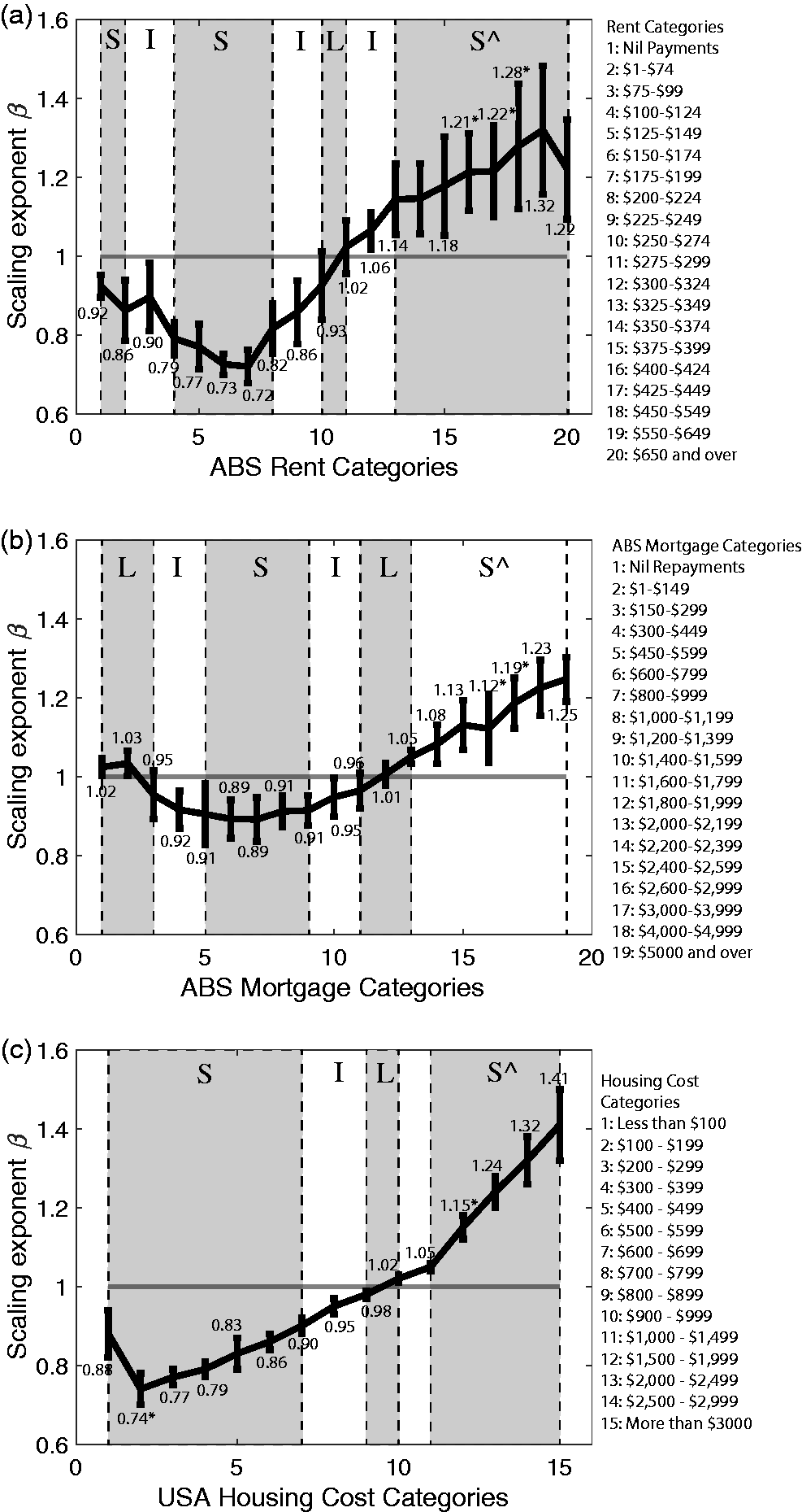

Overall, the housing costs scaling analysis shows that as city size increases, the largest cities have disproportionately high costs of housing with lower numbers of low housing cost dwellings (which scale sub-linearly). This is important to unpack from the normative perspective: if the housing market of the largest cities are only affordable to high-income category residents, and low housing cost dwellings grow sub-linearly with city size, then the low-income residents of the largest cities are not only relatively disadvantaged (losing out in comparison to other high income earners in the same city), but also absolutely disadvantaged (losing out in comparison to other low or middle income earners in other smaller cities). This could cause lower or even middle income earners (some in key occupations like teaching or nursing) to leave the largest cities, an effect that needs to be checked in the future through internal migration patterns. For example, it is known that Sydney regularly records net out-migration losses of key workers to other states and territories in Australia (e.g. −15,900 people in 2014–2015, −23,200 people in 2015–2016 (ABS, 2016)), and part of the reason is the unaffordability of the housing market. The equity implications of this are that the largest cities, filled with the best employment opportunities, the best educational or health care opportunities, and the best amenities and services are then affordable for only the highest earners. Since an entire host of medium and low paying jobs exist to support all primary and secondary economic functions in the large cities, these results show that economic services provided by the low-income residents are needed for a productive city, but affordable housing available for them in the largest cities is scarce.

Geography of distribution and fluctuations: Incomes and housing costs

A geographic evaluation based on LQs that measures the relative concentration of income and housing cost categories in particular cities in comparison to the national average of these categories should echo the scaling analysis: larger cities should show high LQs for higher income groups and higher housing costs, and low LQs for lower income groups and lower housing costs.

Figure 3 shows the LQs for the third lowest income category and the highest income category for all the Australian SUAs and the US MSAs plotted against the log of population. Overall no trend or a very weak trend is seen: at a first glance, there seems to be no trend in response to city size. This was previously reported for per capita intensive measures by Shalizi (2011). However, a closer glance shows that a few large fluctuations or outliers exist. That is, a few small and medium sized cities, marked in grey, show LQ behaviours similar to larger cities: for low-income categories, they show a low LQ, for high income categories, they show extremely high LQs. For example, note in Figure 3(a) the two outliers of Karratha and Port Hedland, that are both mining towns in Western Australia: being the smallest cities in the urban hierarchy, they show the largest concentration of income earners the highest income category.

Figure 3.

Location Quotients (LQs) measuring spatial concentration of income earners in all 101 SUAs of Australia and 384 MSAs of USA. X-axis is the log of city size (total number of households), Y-axis is the LQ of the numbers of households in the (a–b) the third lowest income categories of Australia and USA, respectively, and (c–d) the highest income categories of Australia and USA, respectively.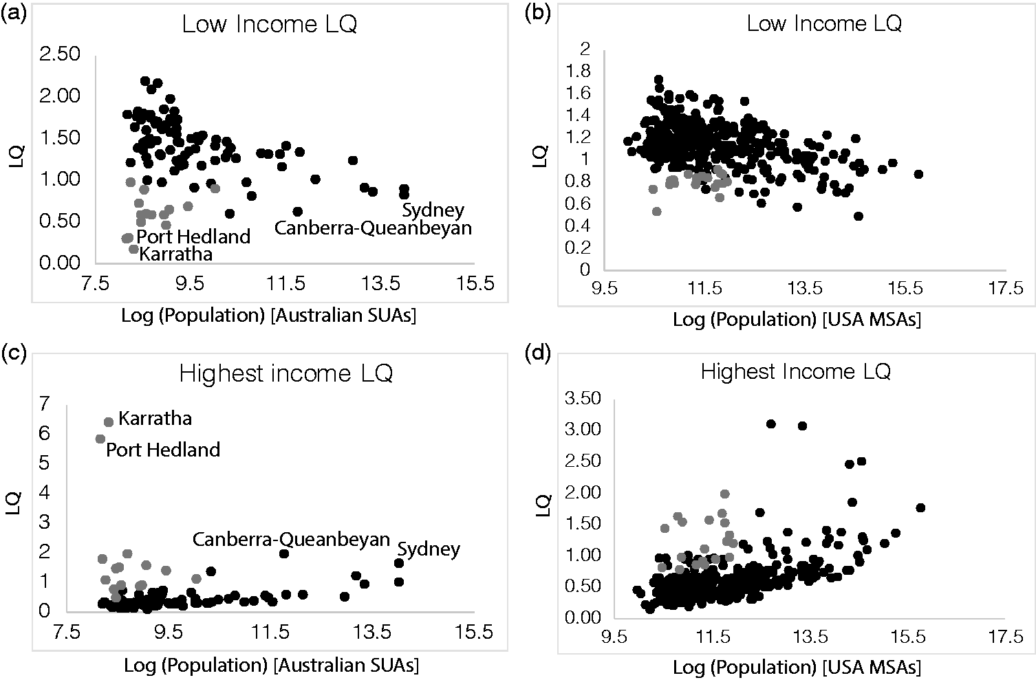

For an exploratory analysis, these large fluctuation outliers are removed from the data set and analysed separately. The top 15 outliers for Australia and the top 20 outliers for USA are extracted out and analysed separately for outlier behaviour (marked in grey). These correspond to cities that have upto roughly one-fourth the population of the largest city (Sydney for Australia and New York–Newark–Jersey City for USA) and show a pattern almost reversed from all other similar sized cities. No statistical principle is applied here for partitioning the data – indeed any other partition is possible. For example, an alternate second partition would be to extract two groups of cities: (a) one group in which higher income categories show high concentration and lower income categories show low concentration and (b) another group with the opposite trend, with lower income categories showing higher concentrations and higher ones showing lower concentration. In such a case, these small and medium sized outliers will be extracted into one group along with all the largest ones. Whatever partitions are chosen, the main aim is to explore the general trend of some of the smaller and medium sized cities emerging as outliers by showing a behaviour similar to the largest cities and quite different to other cities of a similar size, and the reasons for this behaviour.

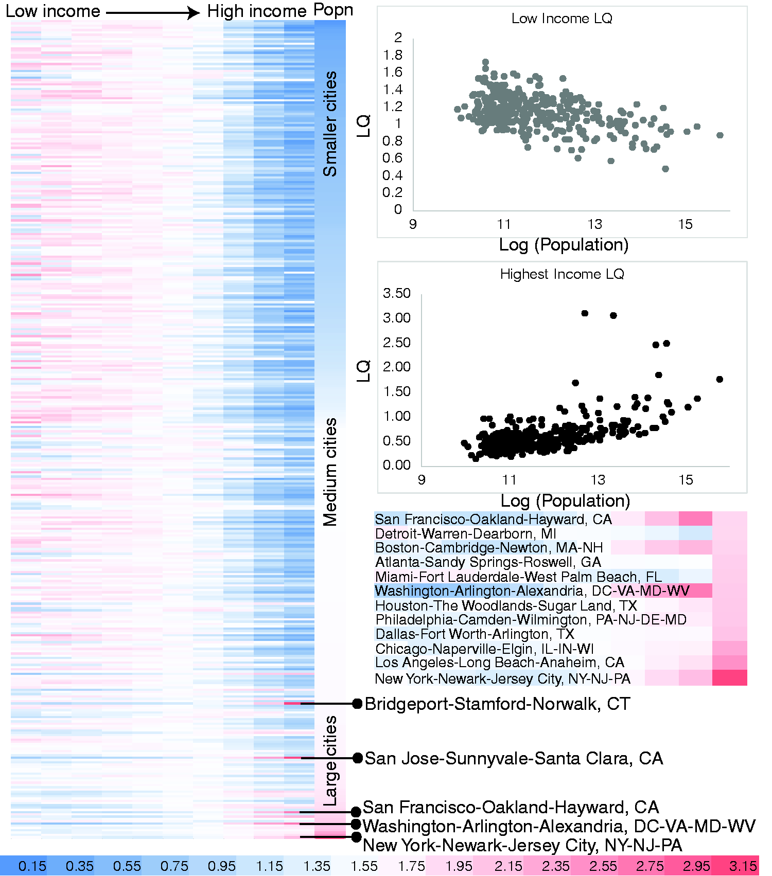
Figures 4 and 5 show the heat map and scatter plots for the LQs for income category concentrations for the SUAs of Australia and the MSAs of the US with the outliers removed. A stronger trend now emerges: small and medium sized cities show concentrations of low to middle income groups, with the higher income groups not showing any specific concentration in these cities. However, the largest cities show high LQs for the highest income groups, and comparatively lower LQs for the lower income groups. Further, Australia and the US both show this universal pattern, but the high-income concentration in the largest cities/metro areas of the US is starker than Australia. The same general trend can be seen in both systems. Sydney, Melbourne, Perth, and Brisbane followed by Canberra and Darwin show very high concentrations of income earners in the highest income categories, with low concentrations of income earners in the lower income categories. The pattern almost abruptly reverses for the large range of other medium and small sized cities. Similarly, the USA analysis shows New York, Los Angeles, Chicago, Dallas-Fortworth, Washington, etc. as the largest metro areas with very high concentrations of income earners in the highest income categories and relatively lower concentrations of low income earners (see inset for top 12 metro areas in Figure 5). Again, the pattern abruptly reverses for most of the smaller and medium sized metro areas. One could hypothesise on a country/region/hierarchy dependent threshold: as cities cross a particular size threshold this concentration effect emerges, whereas it is not observed for most of the distribution.

Figure 4.

Spatial concentration of income earners via Heatmap and scatterplots for Location Quotients (LQs). Rows of heatmap are Significant Urban Areas of Australia (SUAs), columns represent income categories from lowest to highest, last column represents city size (number of households in any income category). Red represents high LQ > 1; blue represents low LQ < 1; white represents LQ ∼ 1. Scatterplots x-axes are populations (log scale), y-axes show LQs.

Figure 5.

Spatial concentration of income earners via Heatmap and scatterplots for Location Quotients (LQs). Rows of heatmap are Metropolitan Statistical Areas (MSAs) of USA; columns represent income categories from lowest to highest, last column represents city size (number of households in any income category). Red represents high LQ > 1; blue represents low LQ < 1; white represents LQ ∼ 1. Scatterplot x-axes are populations (log scale), y-axes show LQs. The largest 12 MSAs (bottom 12 rows of the main heatmap) are shown beneath the scatterplots, with the concentration of high income categories clearly visible.

The results from the LQ analysis for housing costs are shown in Supplementary Figure S1: again, higher housing costs tend to grow by city size, whereas lower housing costs show an opposite trend, corroborating with the scaling analysis. Outliers are removed by the process as described above: it is noteworthy that the process of removing the outliers when separately applied to the rent, mortgage and housing cost data, resulted in nearly the same set of cities being identified as outliers (shown in Supplementary Figure S2). This shows that cities that concentrate high incomes also have high housing costs, regardless of their sizes (small or large).

Unpacking the fluctuations: Specialisation and diversity in small and medium sized towns

Figures 4 and 5 show a general prominent trend, but, as discussed before, some of the smaller and medium sized cities were clear outliers. Supplementary Figure S2 shows small and medium sized SUAs (Australia) and MSAs (US) that are clear fluctuations from the general trend (these clear outliers were removed from the general trend analysis shown in Figures 4 and 5): they show a pattern of geographic distribution similar to the largest cities. In the scaling model, on a log–log plot of the distribution of population against total income, these smaller and medium sized centres appear as large fluctuations on the lower end of the distribution. There can be further analysis done for why these fluctuations occur, but on a case-by-case basis this can be explained via the concentration of specific occupations and industries in these smaller and medium sized centres, and the high correlation of specific occupations and industries with high or low incomes.

If small specialised cities (such as mining towns in Australia) show income distributions (or housing costs) similar in some sense or more extreme behaviour than the largest cities, they should be studied separately. This is because of diversity versus the specialisation characteristics of smaller cities as compared to the largest ones. Smaller and medium sized cities face the possibility of sudden change or death: it is not known or hard to predict what will happen to these cities once the specific economic functions they cater to phase out (for example, mining in Australia), or see massive technological change, even when they lead to very high incomes and housing costs over shorter spans in time. Large cities, by virtue of their diversified or large bases, may not be as temporally volatile.

For example, the largest outliers for Australia shown in Figure 3, Port Hedland and Karratha, are mining centres that agglomerate highly paid workers in the Level 2 Occupation categories of Specialist Managers, Business Human Resource and Marketing Professionals, Design, Engineering, Science and Transport Professionals, Engineering, ICT and Science, Automotive and Engineering Trades Workers, Construction Trades Workers, Electrotechnology and Communications Trades Workers, etc. In these towns, the highly-specialised trades-workers also receive very high incomes (in comparison to professionals and managers, for example). Almost all of the Australian outliers are highly specialised, primarily mining and natural resource extraction cities.

For the US, the outliers show a more diverse occupational and industrial profile. The smaller and medium sized outlier cities with the highest agglomerations of high income earners show concentrations of highly paid occupations such as Computer and Mathematical, Architecture and Engineering, Legal, and Life, Physical and Social Science, but no extremely specialised profile similar to Australia can be seen, at least in this preliminary analysis. One observation emerges though that is common to both countries: an agglomeration of high income categories is frequently accompanied by a parallel low concentration of low income categories.

Conclusions

This paper presented an empirical evaluation of the scaling and geographic distribution of income and housing costs by city size, and tested the specific nature of the large fluctuations shown by some of the smaller and medium sized cities. It was shown that incomes and housing costs scale in a similar way, where the largest cities agglomerate the highest income earners and the highest housing costs, and show relatively lower concentrations of lower income earners and lower housing costs. In contrast, most of the smaller and medium sized cities show the opposite trend. A few small and medium sized cities show trends that correlate with the largest cities, and these appear as deviations or fluctuations in the scaling analysis – a qualitative analysis revealed that this is due to specialisations of economic functions or concentrations of high-paying occupations. A reverse trend is also observed though not as strongly: large cities that do not show high income earner or housing cost concentrations. This is the other end of the fluctuations to be addressed in future work.

The findings from this paper have implications for diseconomies of scale arguments: when does a city grow so large such that negative externalities begin to override positive ones? A new dimension emerges from the analysis presented in this paper: large cities do not seem to be generating negative externalities (say of relative high housing costs) for everyone. Indeed, it is only low or middle income earners who face this disadvantage, since a low-income person in a large, high cost city is worse off both in relative terms in comparison to a higher income earner in the same city, and in absolute terms in comparison to other low and high income earners in smaller or medium sized cities. Hence, the emergent observation that lower and middle income and housing cost categories seem to be concentrated in the smaller and middle sized cities. However, since the largest cities also have the best amenities and services, this results in a situation where the best is available only to the richest.

It is proposed here that one particular diseconomy of scale that is a result of all the others, but one that is not studied widely is inequality. Instead of the narrower term ‘income inequality’, we define inequality as the differential that individuals may face in accessing the resources, amenities and abilities required for their well-being (Sen, 1999). This type of understanding of inequality deeply contrasts with efficiency or performance metrics that are usually considered as given for cities in urban economics. For example, the presence of slum areas in large cities is cited as evidence of their success, since the residents have chosen a higher income in an urban area over a lower income in a rural area (Glaeser, 2012). However, seeing this as a ‘choice’ or ‘social preference’ neglects the observation that for many migrants this may be a forced choice at best, and larger cities may not offer affordable access to resources, amenities or abilities that are needed for their well-being. In contrast, a high-income person in a large city is able to access these resources or amenities with ease.

A parallel view suggests that the trend of higher incomes and higher skills agglomerating in the largest cities may prove beneficial to the lower income or lower skilled residents (Florida, 2004; Glaeser et al., 2001). However, the empirical results in this paper show that larger cities show a disproportionately higher tendency to agglomerate the richest people and housing and a disproportionately lower tendency to agglomerate lower and middle income people and housing. This results in situations where the ability to pay for even fundamental and basic amenities such as housing may be a decisive factor in shaping the well-being and quality of life for residents of large cities, and may exacerbate inequalities of access since the agglomeration of high numbers of people with the ability to pay for a resource may inflate the prices of this resource, thereby taking away this ability from those in lower income categories. In other words, agglomeration of this nature may cause the production of spatial sorting and segregation, leading to social and spatial unfreedoms (Sen, 1999). This affects the ability of communities to have a substantive role in the design and planning of their physical environment (Dong et al., 2013): a community comprising primarily of high income earners is unlikely to make choices that represent the needs and wants of everyone in the income hierarchy, and the non-representation of low income earners in decision making processes is likely to exacerbate conditions such as segregation, polarisation or gentrification. Thus, at the point where a city crosses a certain threshold where incomes of a few and costs of living for all begin to rise disproportionately, such inequality may become a significant diseconomy arising from scaling. Due to the concentrations of high income and high housing costs, largest cities may have a resulting housing market structure that will push out lower and medium income earners, thereby making affordability, diversity, and socio-spatial justice emerge as important urban policy issues.

Supplemental Material

Supplemental material for Urban scaling and the geographic concentration of inequalities by city size

Supplemental material for Urban scaling and the geographic concentration of inequalities by city size by Somwrita Sarkar in Environment and Planning B: Urban Analytics and City Science

Footnotes

Acknowledgement

The author thanks the anonymous referees of this paper for valuable and helpful comments and suggestions.

Declaration of conflicting interests

The author(s) declared no potential conflicts of interest with respect to the research, authorship, and/or publication of this article.

Funding

The author(s) disclosed receipt of the following financial support for the research, authorship, and/or publication of this article: The Henry Halloran Trust, University of Sydney supported the research done in this paper through the funding of the Urban Housing Lab Research Fellowship awarded to the author. The work in this paper is also supported by The University of Sydney's DVC Research Strategic Research Excellence Initiative (SREI-2020) project, “CRISIS: Crisis Response in Interdependent Social-Infrastructure Systems” (IRMA 194163).

Supplementary Material

Supplementary material for this article is available online.

Somwrita Sarkar is Senior Lecturer at the University of Sydney. Her research focuses on the science and modelling of cities using methods from network science, complex systems, physics, economics and geography.

References

ABS (2016) Regional Migration Estimates 2014–15. Available at: http://www.abs.gov.au/ausstats/abs@.nsf/Previousproducts/3412.0Main%20Features72014-15?opendocument&tabname=Summary&prodno=3412.0&issue=2014-15&num=&view= (accessed 9 February 2018).

Arcaute

Hatna

Ferguson

, et al. (2015) Constructing cities, deconstructing scaling laws. Journal of the Royal Society Interface 12(102): 20140745.

Barthelemy

(2016) The Structure and Dynamics of Cities: Urban Data Analysis and Theoretical Modeling, Cambridge: Cambridge University Press.

Batty

(2013) The New Science of Cities, Cambridge: MIT Press.

Beckmann

(1958) City hierarchies and the distribution of city size. Economic Development and Social Change 6(3): 243–248.

Behrens

Robert-Nicoud

(2013) Survival of the fittest in cities: Urbanisation and inequality. The Economic Journal 124: 1371–1400.

Bettencourt

LMA

Lobo

Helbing

, et al. (2007) Growth, innovation, scaling, and the pace of life in cities. Proceedings of the National Academy of Sciences (PNAS) 104(17): 7301–7306.

Bettencourt

LMA

Samaniego

Youn

(2015) Professional diversity and the productivity of cities. Scientific Reports 4: 5393.

Bradbury B (2017) Spatial inequality of Australian men's incomes: 1991 to 2011. In: 27th Australian Labour Market Research (ALMR) Conference, Canberra, Australia, 1–2 December, 2016.

10.

Cottineau C, Finance O, Hatna E, et al. (2016) Defining urban agglomerations to detect agglomeration economies, arxiv preprint: https://arxiv.org/abs/1601.05664.

11.

Dong

Sarkar

Nichols

, et al. (2013) The capability approach as a framework for the assessment of policies towards civic engagement in design. Design Studies 34(3): 326–344.

12.

Florida

(2004) The Rise of the Creative Class, New York: Basic Books.

13.

Fujita

(1989) Urban Economics: Land Use and City Size, Cambridge: Cambridge University Press.

14.

Fujita

Krugman

Venables

(1999) The Spatial Economy: Cities, Regions and International Trade, Cambridge: MIT Press.

15.

Fujita

Thisse

(2013) Economics of Agglomeration: Cities, Industrial Location, and Globalization, 2nd ed. Cambridge: Cambridge University Press.

16.

Glaeser

(2012) The Triumph of the City, New York: Penguin.

17.

Glaeser

Kolko

Saiz

(2001) Consumer city. Journal of Economic Geography 1: 27–50.

18.

Glaeser

Resseger

(2010) The complementarity between cities and skills. Journal of Regional Science 50: 221–244.

19.

Leitao

Miotto

Gerlach

, et al. (2016) Is this scaling nonlinear?. Royal Society Open Science 3: 150649.

20.

Louf

Barthelemy

(2014) Commentary, scaling: Lost in the smog. Environment and Planning B 141: 767–769.

21.

Mameli

Faggian

McCann

(2008) Employment growth in Italian local labour systems: Issues of model specification and sectoral aggregation. Spatial Economic Analysis 3: 343–360.

22.

Marshall

(1920) Principles of Economics, London: Macmillan and Co.

23.

Mori

Nishikimi

Smith

(2008) The number-average size rule: A new empirical relationship between industrial location and city size. Journal of Regional Science 48: 165–211.

24.

Pavan

Baum-Snow

(2013) Inequality and city size. The Review of Economics and Statistics 95(5): 1535–1548.

25.

Pumain D (2004) Scaling laws and urban systems, Santa Fe Institute Working Papers, No. 04-02-002. Available at: https://www.santafe.edu/research/results/working-papers/scaling-laws-and-urban-systems (accessed 9 February 2018).

26.

Pumain

(2006) Alternative explanations of hierarchical differentiation in urban systems. In: Hierarchy in Natural and Social Sciences Vol. 3, Springer Methodos Series. New York: Springer Publishing, pp. 169–222.

27.

Pumain

(2012) Urban systems dynamics, urban growth and scaling laws: The question of ergodicity. In: Portugali

, et al. (eds) Complexity Theories of Cities Have Come of Age, Berlin: Springer-Verlag.

28.

Pumain

Paulus

Vacchiani-Marcuzzo

, et al. (2006) An evolutionary theory for interpreting urban scaling laws. Cybergeo 343: 18.

29.

Sarkar

Phibbs

Simpson

, et al. (2016) The scaling of income distribution in Australia: Possible relationships between urban allometry, city size and economic inequality. Environment and Planning B: Urban Analytics and City Science. . Epub ahead of print 2017. DOI: 10.1177/0265813516676488.

30.

Sen

(1999) Development as Freedom, New York: Oxford University Press.

31.

Shalizi CR (2011) Scaling and hierarchy in urban economies, arxiv pre-print:1102.4101v2.

Supplementary Material

Please find the following supplemental material available below.

For Open Access articles published under a Creative Commons License, all supplemental material carries the same license as the article it is associated with.

For non-Open Access articles published, all supplemental material carries a non-exclusive license, and permission requests for re-use of supplemental material or any part of supplemental material shall be sent directly to the copyright owner as specified in the copyright notice associated with the article.

0.00 MB

0.58 MB