Optimizing bus stop locations for walking access: Stops-first design of a feeder route to enhance a residential plan

Abstract

Feeder buses provide a small but important part of the public transport system by carrying people between residential areas and transport interchanges. A feeder bus to a train station planned in advance will attract new residents of a housing development to use the bus. The bus route can influence the location choice of a buyer concerned about access for children, the elderly or anyone not wishing to drive a car. Our bus route modelling starts with the bus stops – not the route – to be reached from each dwelling by the shortest possible walk. In demand terms, people locating close to bus stops are more likely to use the service than those choosing more distant locations, and the nearby residences have higher values. The stops-first application determines a feeder bus route to enhance an irregular residential plan covering an area of one square kilometre. The planned road and housing lot locations provide the data for calculating the access measure from each dwelling to each potential bus stop, the closest stop being used. A genetic algorithm tests potential bus stops to find demand maximizing locations, the propensity to use the bus being formulated as an exponential (increasing elasticity) function of walking distance. Then a ‘travelling salesman’ genetic algorithm finds the shortest route linking the stops, so that an efficient circuit route is generated for each alternative number of bus stops, ranging from 7 to 11. More stops not only give better access but also increase the route length, so that total accessibility must be assessed against route length. The distribution of walking distances shows most between 150 and 240 metres, with none more than 400 metres. The results indicate that planning policy should require prior design of a bus route to achieve good walking accessibility, so that residents become accustomed to the convenience of using the bus. This study shows that, at the planning stage, estimating a bi-objective model giving a Pareto front between accessibility and route length can reveal a policy compromise that shortens the route with little reduction in expected patronage.

Keywords

Feeder bus route bus stops first optimize stop locations residential planning genetic algorithm dwelling locations walking distance travelling salesman problem

Introduction

This paper makes a case for designing an internal feeder bus route as an integral part of residential planning. The method is to locate bus stops where they give best access from dwellings and then the route is fitted to the stops (cf. Park and Kim, 2010). It is not a matter of incorporating a bus service into an already established locality but prior planning of the service to be part of the total package. If the residential area is effectively a ‘dormitory suburb’ then the potential buyers are likely to perceive an access problem for children and the elderly who need a bus service. At a more general level, there is some evidence that the health of the whole community is promoted by public transport because it is a semi-active transport mode (Durand et al., 2016; Rissel et al., 2012). Furthermore, public transport can reduce the local impacts of air and noise pollution and traffic accidents (Rizzi and De La Maza, 2017).

In real life, public transport agencies tend to find themselves fitting a bus service to a greenfield development only when the area is inhabited. This paper suggests a remedy to the resulting imbalance between land development and the wellbeing of the community.

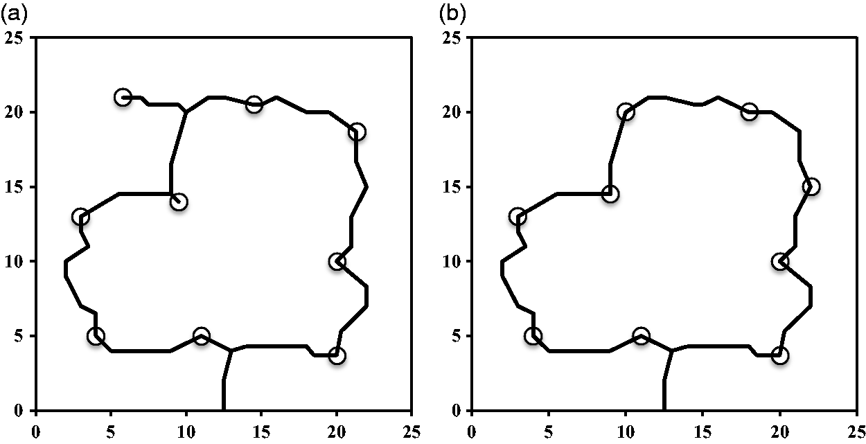
The application has been generated by re-scaling Figure 14 of Sun et al. (2014) to one square kilometre to provide a residential settlement size appropriate for a bus route (Figure 1(a)). Allowing for road space, this gives an average lot size of about 1200 square metres to suit an affluent community but still needing a bus service for the young and the old. The road layout is irregular but with a high level of ‘ringness’, the ratio of the length of roads in circuits to the total length of roads (Erath et al., 2009; Hillier and Hanson, 1984). Compared to a grid layout in the same space, the plan has similar connectivity, measured by straightness centrality, the average ratio of straight line to road distance between residences, and provides for at least as many dwellings.

Figure 1.

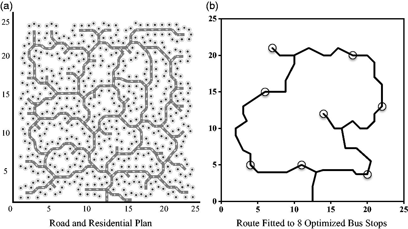
(a) Road and residential plan and (b) route fitted to eight optimized bus stops (scales in units of 40 metres).Source: Figure 1(a) derived from Figure 14 of Sun et al. (2014).

Despite dominance by cars, there would be no traffic problem in this residential precinct because the roads are primarily collectors, and a feeder bus route would serve those unable or not wishing to drive a car. The broad question is the practical feasibility of introducing a bus route giving good access to the planned dwellings and so completing the amenity of the whole development. The angularity and irregularity of the road network in Figure 1(a) provide a rigorous test of feeder bus planning and, at first sight, appear somewhat inimical to the insertion of a bus route. However, a planning bias against the cul-de-sac has limited the number and extent of dead-end branch roads (Sun and Taplin, 2017). Furthermore, the high proportion of roads in shared circuits (ringness) not only gives good access between dwellings but also enables a bus route to serve this planned suburban development with little difficulty.

The main issues are the ease of fitting a bus route to the irregular network, benefit of locating bus stops before fitting the route to them, and finding a compromise between walking accessibility and route length with a bi-objective model. The first step is locating bus stops to maximize accessibility from residential lots. An example is shown in Figure 1(b).

For practical bus service planning, the usual objective is to find a route with good coverage of the area to be served. The planner considers the potential patrons and in residential areas may seek to satisfy the objective of having as many residents as possible within 400 metres of a bus stop (Chia and Lee, 2015; Wang et al., 2016). There may also be shops and other centres to be included in the route but it is noted by Jerby and Ceder (2006) that the shortest route between centres may not be efficient in terms of demand coverage. In a residential area where the bus feeds to a rail interchange and there are no internal centres to be linked, the only service objective is to meet the needs of passengers travelling between their residences and a train station leading to centres of work, shopping, schools, and recreation.

The planning of bus routes has been reviewed by Guihaire and Hao (2008) and by Ibarra-Rojas et al., (2015). Also there are commercial packages for bus planning such as My Route Online™. Whereas the majority of published bus studies deal with large population areas, Nourbakhsh and Ouyang (2012) consider small-scale operations in low demand areas. The bus operates flexibly in a narrow corridor but stops at fixed points, the focus being on system cost and passenger utility. Our study shares the low density character of the area served but seeks a fixed route to fit the dwelling locations.

The review and analysis by Currie and Wallis (2008) show that there are many measures that can increase bus patronage, sometimes by 100% or more. Network structure, service levels, bus priority, vehicles, stop infrastructure, fares, ticketing systems, reliability, passenger information, and marketing are mentioned among a number of effective measures. A point that is relevant to our study is that protracted in-vehicle time is a disincentive to bus travel; Currie and Wallis (2008) note that a reduction of in-vehicle travel time by 10% will increase bus patronage by about 3%.

Frequency of service is most important in bus network design (e.g. Ceder and Wilson, 1986; Cipriani et al., 2012) but timetabling would be an extension of our study which deals with route and stop selection on the basis of walking distances from individual residences. Fan and Machemehl (2006), modelling at the zonal level, take account of ‘long walks’ but this refers to the possibility that a transit user may undertake ‘a long walk … to the neighboring zone and take the bus there’. In their application of GA to bus network optimization, Bielli et al. (2002) identify average walking and waiting time as performance indicators. Chien and Spasovic (2002) specify a demand function that is elastic with respect to service headway, route spacing, and fare. Nourbakhsh and Ouyang (2012) formulate user costs in terms of transfers, waiting, and in-vehicle time but they model passengers being picked up from their exact origins and dropped off at their exact destinations, so that there is no walking time.

Cipriani et al. (2012) assess major bus routes in terms of operator cost, user cost, and unsatisfied demand. The user cost is a weighted sum of travel, access, and waiting times as well as a transfer penalty. The weights are based on previous analysis, and the authors emphasize that the weight on access time is set high to avoid undervaluation of this trip phase.

Coming closer to our approach, El-Geneidy et al. (2014) note that the proportion of the population served by transit is a key performance measure but depends on the definition of the service area. They found that the 85th percentile walking distance to the Montreal bus service is around 524 metres for home-based trips. Verbas et al. (2015) estimate spatial and spatio-temporal elasticities of demand for bus service, making use of the Walk Score™ measure of walkability to assess the likelihood of a stop being used by passengers. This measure is based on distance to the closest amenity in each of several categories including businesses, parks, and theatres (Wikipedia, 2017). Xu et al. (2016) have included ‘walking distances from the community to its nearest station’ as one variable in a function that also includes access time, tolerable travel distance, and tolerable transfer time in order to compute transit accessibility as well as trip distribution.

A survey by Hess (2012) collected information about the perceived and objective barriers experienced by older adults in using transit in Buffalo and Erie County of New York State. He found that older adults do not accurately perceive walking distances but that being close to dense transit networks and frequent service tends to increase their ridership.

Jerby and Ceder (2006) modelled a shuttle bus feeding to a transit station, with patronage projected on a zone basis using number of buildings and a centroid: ‘The demand for trips from a certain road link depends on the walking distances from the land uses around the road to the road itself’. The model selects links to form a circuit that maximizes patronage. To achieve maximum coverage without a long winding route, they imposed a route–time constraint. Thus, route length is not incorporated in the objective but the constraint limits the extent to which the objective is achieved.

Ceder et al. (2015) make a trade-off between accessibility and operation. Their model of bus stop placement takes account of uneven topography in three ways: (1) effect on walking speed, (2) impact on the attractiveness of an access path to a transit service, and (3) effect on acceleration rates at stops. Access is central in our approach which could be extended to take account of topography.

Delmelle et al. (2012) have used an optimizing bus stop location and coverage model taking account of both walking distance from an individual residence to a stop and also transit facility attractiveness. Papers by Chien and Qin (2004) and Johar et al. (2017) also present mathematical models to optimize stop locations, using detailed survey data on bus travel, stopping, and boarding, but the information on access is generalized and the focus in both studies means that distances from individual dwellings could not be taken into account.

Recognizing the indirectness of actual travel, Boscoe et al. (2012) compared the road distance to hospital with direct straight-line distance. Averaged over 66,000 locations in North America they obtained a ‘detour index’ of 1.417. Randall and Baetz (2001) indicate an average ratio of path distance to straight line distance, ‘pedestrian route directness’, from dwellings to central points of about 1.4. Where there are highly indirect road distances to bus stops, access can be improved by the installation of connecting footpaths (cf. Randall and Baetz, 2001). The detour index of 1.4 is used in this paper to convert computed direct distances to walking distances.

The optimizing problem

The primary objective for this study is that residents should have the best feasible access to bus stops (cf. Hess, 2012). A walking distance response function is needed to reflect the increasing disutility of walking further to catch the bus, which means decreasing propensity to use the service (Jerby and Ceder, 2006).

The problem becomes bilevel if the objective is not only to optimize walking accessibility but also to achieve the shortest reasonable route. This has some of the properties of the network design problem as discussed by Yang and Bell (1998) whose two levels were (1) planning extensions and modifications to a road system and (2) maximizing the economic surplus of road users. This study has the primary objective of maximizing the utility of bus stop access and the second objective is minimizing route length.

A bus route and stops to serve a residential area

It is hard to find studies of bus services that clearly put stops first but that could be attributed to past information gaps. School bus planners deal with ‘the joint problem of bus route generation and bus stop selection’, finding the stops to suit the students and then the routes to visit the stops (Schittekat et al., 2013). Determining a bus route for the dwellings in Figure 1(a) is essentially the same as planning a route in an existing suburb where houses are shown in an online map. Although this means that route-first and stops-first planning tend to converge, there is still a difference in principle. Route planning can readily be based on population density (Hsiao et al., 1997) and the study of existing routes by Wu and Murray (2005) considers dwellings as points of potential demand. The latter indicates route planning to serve individual residences; it may fall short of setting the stops to minimize walking distance – before fitting the route to them – but determining the route first and then locating the stops to minimize walking is a comparable approach.

Location at intersections, on the ‘farside’ (downstream), is generally preferred in bus planning guidelines (e.g. BC Transit, 2010; Gold Coast Transit, 2015; Riverside Transit Agency, 2015). Guidelines also indicate that a midblock location may be convenient (e.g. TriMet, Portland, Oregon) in some situations but this possibility was not tested.

The main users of a collector bus are children, aged people, and those who occasionally or frequently choose not to drive. Occasional bus use may be unpredictable but, in addition to regular train commuters, the young and old users can be projected. School bus planners normally have the information they need (Park and Kim, 2010), there is documentation on aged people and, in Australia, passes are issued to seniors by public transport agencies (e.g. PTAWA, Public Transport Authority of Western Australia, 2018; Seniors SmartRider). Planners might also seek access to the emerging but somewhat contentious data sources generated by personal computing devices especially mobile phones. All of these are helpful but children grow up and parents get older, whereas a bus route is planned for the long term and changing demography would rarely be enough to change an established route.

New site development is an opportunity to attract and consolidate bus patronage as new residents arrive but the only data are road and dwelling locations, as simulated in this study. A bus route planned in advance can influence the location choices of some intending residents and others are likely to take note of the route and stops. Wang et al. (2015) have shown that property values near to bus stops rise above the values of surrounding properties. The logic of people locating close to bus stops being more likely to use the service than those choosing more distant locations partly underlies the formulation of the walking distance response function in the next section. The access measure is calculated from each dwelling to each potential bus stop, the closest stop being used.

Potential bus demand with respect to walking access distance

In his study of pedestrian access to the BART rail system in the San Francisco area, Cervero (2001) found that walking was the dominant means of station access up to about a kilometre. However, the issue for this study is not the choice of access mode but the effect of walking distance on the decision to make a bus trip. The disutility of walking to a bus stop as distance increases and its effect on potential trips can be approached in terms of the patronage decay functions considered in a number of studies of walking to public transport (Chia and Lee, 2015; Durand et al., 2016; Gutierrez et al., 2011; Hess, 2012; O’Sullivan and Morrall, 1996; Wang et al., 2016; Zacharias and Zhao, 2018; Zhao et al., 2014).

Topics in these studies have included factors in the acceptability of walking, inferences from smart card data, magnitude of pedestrian catchments, use of walking data in public transport models, distribution of walking distance, and health impacts of walking to transit. A specific distance decay function is presented by Zhao et al. (2014) to reflect ‘the deterioration of transit use due to increasing walking distance’. 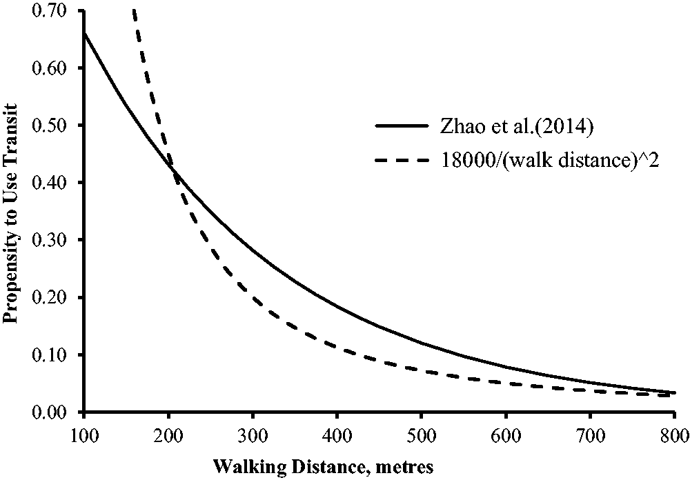The function they estimate, using data from southeast Florida, is $y = 1.0126 E x p (- 0.0013 x)$ , where x is walking distance, in feet, to a transit stop and y is a normalized measure of response, ranging from 0 to 1. This function (in metres instead of feet) is shown in Figure 2. A scaled inverse of the square of distance, which was an option for calculating walking disutility, is also shown in Figure 2; the effect of applying it to our problem is presented in ‘Changes in stop locations and access if squared distance is used to represent disutility’ section, for comparison.

Figure 2.

Alternative representations of the declining acceptability of walking to transit.

Using squared distance as the disutility of walking to catch a bus is equivalent to a demand elasticity of −2.0 at all distances whereas the function of Zhao et al. (2014) gives increasingly elastic demand as the distance increases. Glaister and Graham (2005) showed that this type of function is convenient for estimating changing elasticity $(\frac{\partial y}{\partial x} * \frac{x}{y})$ . The elasticity of demand with respect to walking distance is −0.4 at 100, −1.7 at 400, and −3.0 at 700 metres. This means growing unwillingness to walk to the bus stop, which is intuitively plausible as well as having an empirical basis. Our calculation of propensity to use transit, which is effectively potential demand for bus with respect to walking distance, uses a simplification of the Zhao et al. (2014) function, transformed to metres (equation (2)).

A bus route for the planned residential area

There are three stages in the bus route determination:

Optimally locate each bus stop at an intersection in the planning area.

Find the shortest route linking the bus stops determined in Stage 1.

Determine the preferred number of stops and estimate the Pareto front between non-dominated solutions for maximum propensity to use bus and minimum route length.

Stage 3 is deferred to ‘Efficient bus stops and estimation of the Pareto front’ section where the Pareto front is used to find a shortened route that does not seriously reduce total propensity to catch the bus.

The following notation is used:

i ∈ I: index and set of 485 dwelling nodes

j, k ∈ J: index and set of intersections that are potential bus stops

r ∈ R: index and set of road sections between bus stops

x_i, y_i: location coordinates of dwelling i

x_j, y_j: location coordinates of potential bus stop j

d_ij: direct distance between dwelling node i and potential bus stop at intersection j $d i j = \sqrt{{(x_{i} - x_{j})}^{2} + {(y_{i} - y_{j})}^{2}}$

e : entry–exit to circuit bus route

δ : length of circuit bus route beginning and ending at entry–exit e

c_jk: road distance between bus stop at intersection j and bus stop at intersection k

η_ij: walking interaction between dwelling i and bus stop at intersection j

Decision variables:

K: set of t chosen bus stops (K ∈ J and 7 ≤ t ≤ 11)

K_{j} = {\begin{array}{l} 1 if potential bus stop at j is in set of chosen bus stops K \\ 0 otherwise \end{array}

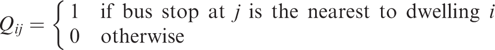
Q_ij: assigning each dwelling to the nearest bus stop j ∈ K

Q_{i j} = {\begin{array}{l} 1 if bus stop at j is the nearest to dwelling i \\ 0 otherwise \end{array}

The Stage 1 model to optimally locate bus stops is

Maximize ζ = \sum_{i \in I} \sum_{j \in J} η_{i j}

(1)

Subject to η_{i j} = ⌊ E x p (- 0.004265 d_{i j}) ⌋ K_{j} Q_{i j}

(2)

Thus, the first stage finds the best locations for the t bus stops by maximizing total utility ζ, which also means minimizing walking disutility. The objective is the sum of the propensities to walk from each dwelling i to the nearest bus stop at j. Equation (2) results in one only calculation for each dwelling being included in summation (1). There are 43 intersections (excluding 16 minor ones) in the network, which provide the feasible bus stops.

Stage 2 is a travelling salesman problem (TSP) to find the shortest route linking the chosen bus stops; it can be formulated as an integer program (Potvin, 1996; Wikipedia, 2018)

r_{j k} = {\begin{array}{l} 1 if the route goes from bus stop at j \in K to bus stop at k \in K \\ 0 otherwise \end{array}

Minimize L = \sum_{j = 1}^{t} \sum_{k \neq j, k = 1}^{t} c_{j k} r_{j k}

(3)

Subject to \sum_{j = 1, j \neq k}^{t} r_{j k} = 1; there is an incoming link to each stop from only one other stop

(4)

\sum_{k = 1, k \neq j}^{t} r_{j k} = 1; from each stop there is a departure link to exactly one other stop

(5)

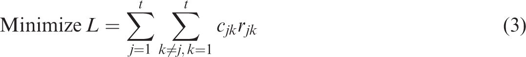
Solution by linear programming requires added constraints to prevent sub-tours but, as Potvin (1996) shows, these are not required when solution is by genetic algorithm (GA).

The entry–exit e is not on the circuit but adds to the route length

δ = (L + 2 c_{t e}) to form the full circuit (e, K_{1} \dots, K_{j} \dots K_{t}, e)

(6)

Thus, Stage 2 minimizes the length of the total route δ travelled by a bus entering the area at entry–exit e, calling at each of the t stops and completing the circuit by returning to entry–exit e. The locations of the bus stops K have already been determined in the first stage. There is a separate application for each number of stops (7, 8, 9, 10, 11). This range has been chosen so that the average spacing between stops lies between 400 and 700 metres. The spacing outcomes are presented with the results.

Although the search in Stage 2 is to find the optimal circuit route, it is recognized that an in-and-out route could be designed to reach the final stop over a route serving all stops and then returning by the same route. This alternative is solved by a restricted form of problem (3) optimized for each number of stops and compared with the optimized circuit route.

There is also the implicit constraint that it should be a ‘reasonable route’. Some passengers may enjoy travelling around the circuit, a ‘valued activity’ as discussed by Banister (2008) but, to satisfy passengers wanting a moderately short trip, the operational solution is to alternate the bus service direction between clockwise and anticlockwise circuits.

Stage 1: Determining the bus stop locations

The problem is to select bus stops from the 43 possibilities by maximizing the sum of propensities to use bus, ζ, from the 485 residential centroids – the dots in Figure 1(a). This is without regard to the eventual bus route. The evolutionary option in the Excel Solver was tested as a way of seeking optimum locations but was found to reach inferior solutions. The only other type of solver considered is GA which has been used extensively for transport and location problems, particularly road investment and maintenance as discussed in Qiu (1997), Taplin and Qiu (2001) and more extensively in Taplin et al. (2005). Road investment and bus stop location searches are integer problems, for which GA is well suited. Much of the computation time in these studies and the current one are required to calculate the value of the objective function. In a different field, the use of GA to design spatially cohesive nature reserves is reported by Delmelle et al. (2017).

The GA makes a systematic search to find the optimum solution, starting with a population, usually between 50 and 100, of randomly drawn feasible solutions. Each is represented in a chromosome comprising the set number of randomly selected bus stops at intersection locations. The search produces consecutive generations of solutions by both random changes (mutations) to individual bus stop locations and crossover operations. In the latter, corresponding segments in two randomly chosen chromosomes are exchanged, with any duplication being repaired, to produce two new chromosomes. The population in each generation is limited to the initial number. This procedure leads to combinations of groups of stops that have already tended to increase the objective value. However, all operations are sufficiently random to ensure that the search space is well covered and premature convergence to inferior solutions is generally avoided. The GA parameters used in this study are:

Population: 60 chromosomes

Crossover rate: 0.6

Mutation rate: 0.25.

In Table 1 (top left part of the computing spreadsheet for seven bus stops), the distance is found from each dwelling location to the nearest stop. Equation (2) applied to this minimum distance gives the Bus Use Propensity. The task of the GA (result shown in the lower part of Table 1) is to find the set of bus stops that maximize the total propensity to use bus. Convergence of the Evolver GA was slow in some cases so that the number of ‘trials’ was set to 30,000. Sometimes, there were changes towards the end of these, so that more were run to give some assurance that the search had converged on the best solution.

Table 1.

Portion of spreadsheet to compute the sum of household bus use propensities: seven stops.

Location			Calculated distance from dwelling location to bus stop (units of 40 metres)								Bus use^a	Wtd by
X	Y	Dwellings	Stop 1	Stop 2	Stop 3	Stop 4	Stop 5	Stop 6	Stop 7	Minimum	propensity	dwellings
1	1	1	17.26	17.03	24.19	25.50	20.62	12.17	5.83	5.83	0.370	0.370
1	2	1	17.12	16.40	23.71	24.76	19.65	11.18	5.39	5.39	0.399	0.399
1	5	1	17.03	14.76	22.47	22.67	16.76	8.25	5.10	5.10	0.419	0.419
1	6	1	17.12	14.32	22.14	22.02	15.81	7.28	5.39	5.39	0.399	0.399
1	8	1	17.46	13.60	21.59	20.81	13.93	5.39	6.40	5.39	0.399	0.399
1	9	1	17.72	13.34	21.38	20.25	13.00	4.47	7.07	4.47	0.466	0.466
1	10	1	18.03	13.15	21.21	19.72	12.08	3.61	7.81	3.61	0.541	0.541
1	11	1	18.38	13.04	21.10	19.24	11.18	2.83	8.60	2.83	0.617	0.617
1	12	2	18.79	13.00	21.02	18.79	10.30	2.24	9.43	2.24	0.683	1.366
… followed by 399 more rows (with 475 more dwellings)
										Total propensity to use bus		274.206
	X	Y	Point
Bus stop locations at the points chosen by GA (not ordered)
Stop 1	18	4	55
Stop 2	14	12	31
Stop 3	22	13	29
Stop 4	18	20	13
Stop 5	6	21	5
Stop 6	3	13	27
Stop 7	6	4	52

^aEquation (2) applied to the minimum distance.

Separate solutions are obtained for 7, 8, 9, 10, and 11 bus stops (Figure 1(b) shows the result for 8). The number of dwellings within 200 metres (direct distance) of a bus stop was also calculated but this did not influence the objective function. This distance is shorter than the conventional 400 metres walking distance but, as discussed, 200 metres in a straight line is equivalent to about 280 metres of walking distance (Boscoe et al., 2012; Randall and Baetz, 2001).

Stage 2: Linking bus stops into routes

The bus stops selected by the GA in Stage 1 are located at road intersections but are not ordered. They are to be linked and ordered into segments of the existing roads. As indicated, this is a ‘travelling salesman’ problem to find the shortest route starting at the entry–exit and completing the circuit at the same point. The TSP can be solved by various algorithms but GA has been widely used; in this case, the GA used in Stage 2 can be conveniently integrated with the GA of Stage 1 when the bi-objective Pareto frontier is estimated in Stage 3 (‘Efficient bus stops and estimation of the Pareto front’ section).

An ‘order’ procedure rearranges and links the bus stops at the fixed points determined in Stage 1, the solution being based on a matrix of road distances between these stops. The alternative in-and-out route to the final stop and returning by the same route is solved by a restricted form of TSP. The entry–exit is one end of the route and the other end is at the most distant bus stop. The two sets of results are compared in Table 2.

Table 2.

Comparison of circuit routes with identical in-and-out routes.

Number of stops	Circuit route, total length (kilometres)	Identical in and out, total length (kilometres)	Difference (kilometres)	Circuit length as per cent of identical in and out
7	4.95	8.92	3.99	56
8	4.95	9.08	4.13	55
9	4.51	9.22	4.71	49
10	5.62	9.51	3.89	59
11	5.62	9.56	3.94	59

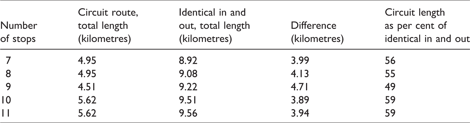
The route layout for 11 stops in Figure 3 provides visual comparison of a circuit route with an identical in and out; the circuit, on the left-hand side, is somewhat less convoluted than the inward and outward bus trip by the same route and is 59% of the total length (last column of Table 2). The layouts in Figure 3 are simplified, with some bends made linear, but distance calculations follow the detailed road layout in Figure 1(a). Results for 7, 8, and 10 bus stops are shown in online supplemental material and nine-stop layouts are considered in ‘Efficient bus stops and estimation of the Pareto front’ section. The optimized 10 stop circuit has been modified and made continuous to avoid having extensive branches, at a distance cost of only 17 metres.

Figure 3.

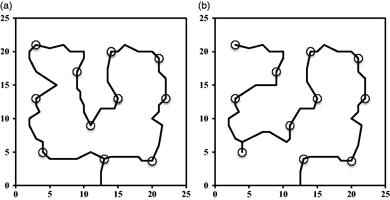
Comparison of (a) circuit with (b) identical in and out: 11 stops (scales in units of 40 metres).

Location and access results by number of bus stops

Table 3 shows data generated by maximizing propensity to use bus with each number of bus stops and Table 4 presents the relative patronage implied for each stop. The bus stop spacing in each case (Table 3) is within usual practice. There is no universal standard, as illustrated by Tirachini (2014) who shows a range of average spacing in cities around the world from 250 to 1750 metres, with a median value for 37 systems of 550 metres. One system, Transfort (2015) recommends a range of 400–800 metres on suburban local routes in the Fort Collins area of Colorado.

Table 3.

Results of optimizing bus stops and then fitting the route.

Number of stops	Sum of propensities to use bus, ζ^a	Circuit route length (kilometres)	Average spacing between stops^b (metres)	Average walking distance^c (metres)	Dwellings within 200 metre radius^d of a stop (%)
7	274.2	4.95	656	199	76
8	285.3	4.95	574	183	84
9	293.4	4.51	461	173	91
10	301.4	5.62	526	165	95
11	308.2	5.62	434	157	96

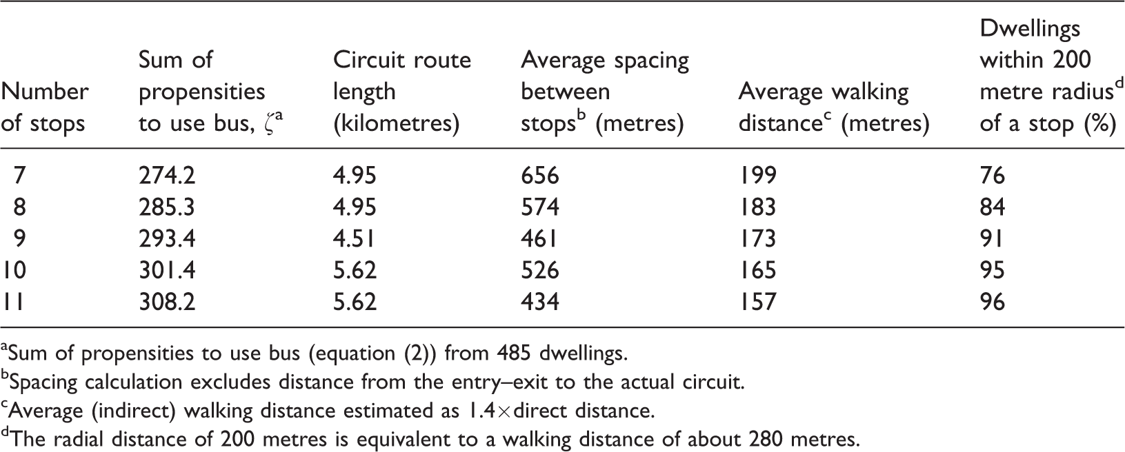
^aSum of propensities to use bus (equation (2)) from 485 dwellings.

^bSpacing calculation excludes distance from the entry–exit to the actual circuit.

^cAverage (indirect) walking distance estimated as 1.4×direct distance.

^dThe radial distance of 200 metres is equivalent to a walking distance of about 280 metres.

Table 4.

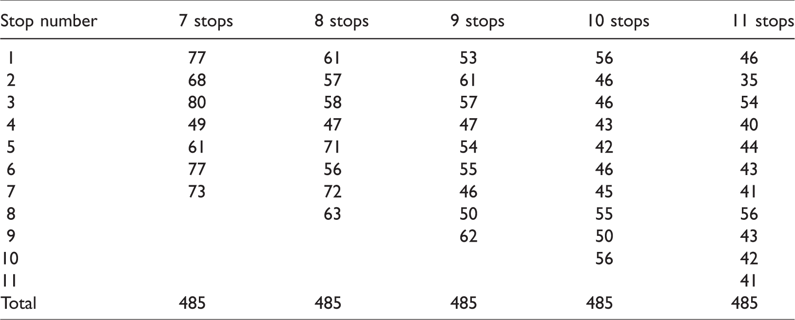
Number of dwellings associated with each bus stop.

Stop number	7 stops	8 stops	9 stops	10 stops	11 stops
1	77	61	53	56	46
2	68	57	61	46	35
3	80	58	57	46	54
4	49	47	47	43	40
5	61	71	54	42	44
6	77	56	55	46	43
7	73	72	46	45	41
8		63	50	55	56
9			62	50	43
10				56	42
11					41
Total	485	485	485	485	485

The estimates of the aggregated propensities to use the bus in Table 3 give some indication of the numbers that might use the bus service and also indicates the increasing utility of the reduced walking distances. The last column of Table 3 shows the increasing proportion of dwellings within a radius of 200 metres as the number of bus stops is increased.

Table 4 shows each bus stop and the number of dwellings having their shortest distance to it. The stops are shown in sequence but a particular stop number may be at different locations on the different routes. Each of the 485 dwellings is counted once in every case. The implications are indirect because one cannot predict how many bus trips would be generated by individual households. However, the number of dwellings associated with each stop has been fairly evenly distributed by the algorithm and this suggests that there would not be any concentrations of travellers at particular stops. For comparison, and ignoring the population disparity, El-Geneidy et al. (2014) found service gaps across large areas of Montreal and redundant stops on some routes, together implying uneven distribution of travellers to stops.

Table 5 presents further inferences, using seven-stop results as the basis for comparison. The seven-stop route gives not only relatively low bus use propensity but also the proportion of dwellings within a direct distance of 200 metres is low (Table 3). At the other extreme, the 11-stop route (Figure 3) with relatively closely spaced stops might be considered tortuous and time consuming by passengers. In making a trade-off between accessibility and route length, there is not only bus operating cost to consider but also the reduced level of service resulting from protracted in-vehicle journey time. A wandering bus might serve a lot of dwellings but could be painfully slow.

Table 5.

Projected impacts of accessibility and route length.

Number of stops	Average propensity to use bus^a	Change in propensity to use bus (walking acceptability)	Route length (kilometres)	Estimated impact of route length on patronage^b
7	0.565	(base)	4.95	(base)
8	0.588	4.1%	4.95	–
9	0.605	7.1%	4.51	2.7%
10	0.621	9.9%	5.62	−4.1%
11	0.635	12.4%	5.62	−4.1%

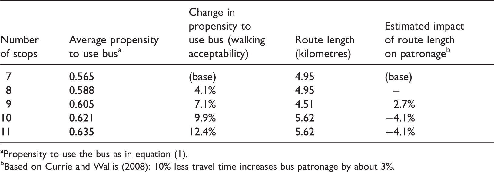
^aPropensity to use the bus as in equation (1).

^bBased on Currie and Wallis (2008): 10% less travel time increases bus patronage by about 3%.

Part of the reason for using the Zhao et al. (2014) relationship is that it reflects ‘the deterioration of transit use due to increasing walking distance’. In other words, the walking acceptability indicated by Figure 2 represents relative bus patronage. The third column of Table 5 shows the projected improvement in propensity, due to improved walking acceptability, as the number of stops is increased.

However, more stops generally mean a longer route. The last column of Table 5 indicates the offsetting effects of increased route length, using the Currie and Wallis (2008) finding that a reduction of in-vehicle travel time by 10% will increase bus patronage by about 3%. In-vehicle travel time is taken to be proportional to route length. In the 10-stop and 11-stop cases, increased route (and trip) length are projected to generate negative patronage effects but probably not enough to offset the large accessibility benefits of more stops. The eight-stop and nine-stop routes would give smaller but appreciable access benefits. The passenger experience would also include the frequency of service, to be decided after the route and stop configuration has been determined.

The possibility of route-first planning can now be considered in the light of the stops-first results. The circuits in Figure 3 and online supplemental material suggest that a general circuit route could be found around the residential precinct, located between about 120 and 250 metres from the perimeter. The difficulty is that internal dwelling locations call for at least one bus stop if reasonable walking access is to be achieved. Solutions to this difficulty have been a deviation to the interior of the area (7-stop, 8-stop) or a substantial loop (10-stop, 11-stop) but these are based on optimal location of stops initially. While route-first planning might be able to deal with this in a reasonable fashion, it is not apparent that such an approach would have any advantage over the rigorous stops-first method.

The access outcome for individual users

The distribution of expected walking distances is presented for the eight-stop case in Figure 4. These are the indirect walking distances from the individual dwellings estimated as direct distance multiplied by the ‘detour’ factor of 1.4 (cf. Boscoe et al., 2012; Randall and Baetz, 2001). The average is 183 metres, as shown in Table 3.

Figure 4.

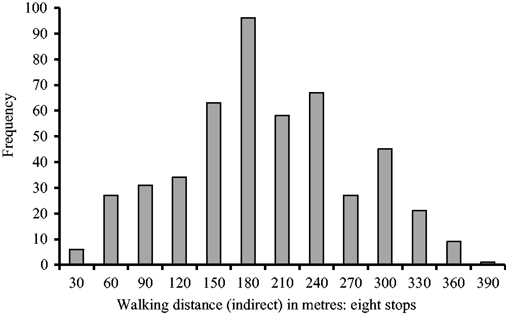
Distribution of modelled walking distances from 485 dwellings to nearest of eight bus stops.

Unlike population or survey data, the distribution in Figure 4 is entirely the result of computation, although the function representing propensity to catch the bus with respect to walking distance is chosen to reflect previous observations of behaviour (Zhao et al., 2014). In effect, the distribution is the outcome of a series of modelling procedures and constraints:

Residential layout modelling, with the result shown in Figure 1(a).

Choice of the distance and propensity function (equation (2)) based on walking acceptability that becomes increasingly elastic with respect to distance (Figure 2).

The search procedure to find the bus stop locations. Of the 43 potential locations at intersections, across all bus models, 28 were fully evaluated by the algorithmic searches.

The bus stops were selected to minimize walking disutility but the potential bus stop locations were constrained by the road layout (Figure 1(a)).

Incoming residents who consider using the bus would rarely find that they would need to walk as much as 400 metres, the conventional planning distance, and would generally have to walk about half that (Figure 4).

Changes in stop locations and access if squared distance is used to represent disutility

In ‘A bus route and stops to serve a residential area’ section, squared distance, representing the disutility of walking distance, was considered as a possible objective to be minimized in the search for bus stop locations. It was rejected on the grounds that its constant elasticity failed to reflect the increasing disutility of every additional metre of walking distance. When squared distance was tested as a disutility function there were five changes of stop location in the 11-stop case and four in the 10-stop but no change for 7, 8, or 9 stops. The location changes for 11-stops are shown in Figure 5.

Figure 5.

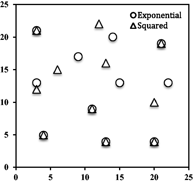
Changes in bus stop locations when squared distance is used as penalty: 11 stops.

The choices are constrained by the available locations but with the exponential function the increasing elasticity of the propensity to use bus imposes relatively more pressure to achieve shorter walking distances. Using disutility calculated as squared walking distance would result in a greater average walking distance of 2.2 metres or 1.4%. This is not due to the inverse specification, as a disutility, but to the different underlying forms of the two functions illustrated by Figure 2.

Efficient bus stops and estimation of the Pareto front

Results of the maximum utility selection of bus stop locations are plotted against route length in Figure 6. The nine-stop solution dominates the seven-stop and eight-stop because it has a shorter route and gives greater utility (propensity to use bus). Also the 11-stop dominates the 10-stop. The solid line links the two efficient solutions, 9 and 11 stops; the latter gives 5% more utility but its 24.6% longer route is deemed to make it inferior to the nine-stop alternative. Thus, the results in Figure 6 facilitate a choice between alternative numbers of stops but these results are obtained by maximizing total propensity to use the bus, with the route being the best fit to the stops regardless of its length. In planning and management terms, there is also a trade-off between maximum accessibility and minimum route length; this is assessed by jointly optimizing the two objectives.

Figure 6.

Optimized access utility and resulting route length for 7–11 bus stops.

Joint optimization

We take the nine-stop case which has been optimized for utility only and seek the non-dominated solutions for reduced route length and the correspondingly decreased utility, thus marking out the Pareto front linking non-dominated solutions. At each solution on the front, one objective cannot be improved without sacrificing some of the other. Kovacs et al. (2015) consider multiple objectives in vehicle routing and delivery problems but note that the objectives are often reduced to only two. Their review shows that finding a trade-off between routing cost and consistency of customer service is a pervasive problem. Across all fields, estimating the front with a bi-objective model is generally difficult and becomes extremely difficult in a case such as designing spatially cohesive nature reserves by optimally linking irregular patches of habitat (Delmelle et al., 2017). Estimation methods tend to vary by class of problem; ours has an irregular spatial layout but the roads are linear, with potential bus stops limited to intersections.

The service in the bus layout problem differs radically from those considered by Kovacs et al. (2015) in that our ‘customer service’ is based on walking access to the vehicle whereas their services are provided by vehicles delivering consignments to customer locations. The procedure illustrated in Figure 7 is in two steps, starting with a form of the epsilon constraint method (Haimes et al., 1971) whereby one of the two objectives is converted into a systematically varied constraint on the optimization of the other objective. In the bus application, route length is gradually reduced by changing the stop locations, total length being minimized each time. Once the stops have been set at feasible locations, the utility is automatically maximized through the reallocation of each household to the nearest stop, as shown in Table 1. The results below the front in Figure 7, as well as two on the front, have been calculated in this way. The interval sizes are determined by the road layout and intersections, so that they are not equal.

Figure 7.

Estimated Pareto front between utility and route length for nine bus stops.

Finding points on the Pareto front

The joint optimization integrates the search for bus stop locations to maximize utility of customers walking to stops and the search for the shortest feasible route. The solutions are found by a succession of GA applications, each starting from one of the better epsilon constraint results. This is similar to the procedure of Malik (2012) who could only get a non-dominated sorting algorithm (NSGA-II), for his manufacturing and customer service problem, to work by using the epsilon constraint solutions as starting values. It is also similar to the two-phase heuristic of Delmelle et al. (2017).

The steps in the search for points on the Pareto front in the nine-stop bus route problem are as follows:

Choose successive sets of nine stops that give decreasing route lengths; determine the utility objective outcome for each set – these are the epsilon constraint solutions.

Use the utility maximizing GA solving method to shift one of the better epsilon constraint solutions to a superior bi-optimization position, thus:

Set the goal of the GA to increasing the utility objective value, which it may be able to do by replacing one or more of the nine bus stop locations.

However, a soft constraint is set on route length, either at the previous length or shorter: any excess length causes an increasing penalty to be applied to the objective value.

The GA may replace a stop location to improve utility but if this causes an increase in route length then it will incur the increasing penalty.

On completion of the run, the software removes the penalty from the objective value but any increase in route length is retained.

If a non-dominated solution S₁ is achieved then it forms a point on the Pareto front; however, if it is dominated by a subsequent solution S₂ the adjusted Pareto front will then pass above S₁.

Apply steps 1 to 3 to the next epsilon constraint solution.

In step 2, the sequence of bus stops is entered in the layout for the TSP and route length is calculated, but the stop locations are also carried into the household utility calculation (as in Table 1) and the GA solving method is maximizing access utility, not minimizing route length. The soft penalty on route length is (10×(EXP(DEVIATION/100)−1)) which is deducted from the utility objective during computation whenever the length limit is exceeded. A hard (rejection) constraint is not used because it would lose the evaluative effect of the soft constraint on route length and, more broadly, cause loss of information (Michalewicz, 1995). Although the soft penalty is not retained in the final objective value it is important in the computation because it makes route length a scarce resource, to be used as efficiently as possible in generating utility. The penalty multiplier of 10 occasionally allows the length limit to be exceeded by no more than 5 metres in the final result – a small position shift on the Pareto front. Nevertheless, the constraining effect of route length on the joint problem is comparable in importance to the effect of bus stop locations.

In practice, the method is like a search for the shortest path but, unlike the TSP, a bus stop can be replaced. The effect of structuring the problem in this way is that the GA is free to test any bus stop location but the change will only be accepted if the replacement stop fits reasonably into the sequence position of the stop being replaced. A change that does not fit well in the sequence will lengthen the route and so be discarded by the GA.

Although the analysis is conducted in terms of utility and route length, Figure 8 indicates that route structure has considerable influence. Whereas the accessibility maximizing circuit for nine bus stops has two short branches (Figure 8(a)), requiring the bus driver to deviate and then reverse to rejoin the main circuit, the shorter route does not have these deviations. In fact the point (3.93, 286.6) on the Pareto front in Figure 7, summarizing the route in Figure 8(b), results mainly from the deviations on the initially optimized route (Figure 8(a)) being stripped away. Thus, Figure 8(b) provides one compromise answer to the problem of finding a reasonable bus driving configuration that preserves as much utility as possible. With reference to the utility maximizing route (Figure 8(a)), there is a 13% reduction in route length for only a 2.3% reduction in utility.

Figure 8.

Maximum utility compared to a compromise with route length: nine stops. (a) Route fitted to utility maximized stops, route length: 4.51 kilometres; utility: 293.4 and (b) a compromise on the Pareto front, route length: 3.93 kilometres; utility: 286.6.

Should there be a need to shorten the route further then the lowest point (3.47, 275.2) that has been estimated on the Pareto front in Figure 7 offers a 23% reduction in route length for only a 6.2% reduction in utility. Although a shortened route means poorer walking access, this would be partly offset by the favourable response to the reduced travel time (Currie and Wallis, 2008).

Planning and policy implications

Whereas bus route planning is normally concerned with an existing urban or suburban area, this study deals with new residential development. Where the development is undertaken by a private corporation, it is subject to planning controls and the planning authority might require the developer to demonstrate the feasibility of adding a bus route. An irregular layout may well be contemplated, particularly in irregular terrain or where there is intrusion by natural features or specified parkland. These are well suited to the automated planning method which has been shown to generate a relatively large number of lots with good accessibility (Sun et al., 2014).

The policy issue motivating this study is the need to ensure that a well-planned bus service is available to people settling in the newly developed suburban area. In a car-dominated society, the young and the old are likely to need a bus service and there are also car owners and drivers who prefer or have good reason to use public transport. The situation contemplated in this paper is a bus service feeding to a train station where restricted space may limit the park-and-ride option for commuters, so that they would find it more satisfactory to take the bus to the station. But such commuters would be relatively intolerant of a long winding bus ride, so that cutting route length from 4.5 to 3.9 kilometres (Figure 8) might add substantially to patronage. The Pareto front to assess route length against general accessibility thus becomes a key resource in bus route planning.

The focus of the study has been on maximizing walking access from residences but there are two caveats. One is that, although a shortened bus route would reduce walking accessibility, it might be good policy in attracting commuters. As demonstrated, a reasonable compromise can be located on the Pareto front. The other caveat is related to the selection of a dwelling location by an incoming buyer. Should a buyer have no interest in bus access, and possibly be repelled by high land price close to a bus stop (Wang et al., 2015), then they could be expected to buy a housing lot well away from a bus stop as shown in Figure 4, about a 400-metre walk from a stop. That is still within the conventional range but a modified bus route, as in Figure 8(b), extends the reasoning. That route modification would leave a relatively bus-free precinct in the north-west corner of the development which could attract residents who are indifferent to bus access or even slightly averse to it.

A broader perspective in this paper has been the balance between the aims of the land developer and the wellbeing of the community. The goal of fitting a bus service to a greenfield development before it is inhabited implies a policy instrument or planning control requiring the developer to show the feasibility of a bus route. The regulation could be couched in terms of total accessibility as calculated here. Any low to medium density residential development plan could have the method applied to it, subject to a specified minimum of accessibility, but also the potential bus operator would have to deal with costs and frequency and should be consulted on the route layout.

Whatever the process, the main thing is to establish the bus route as early as possible after the road and residential layout is determined – the two might even be done in conjunction. Within the route modelling there would also be practical details, particularly intersection geometry. Bus drivers are often faced by difficult turns, which can include small traffic circles, and improvements at the planning stage would ensure an enhanced outcome.

Finally, the suggested planning control should be administered flexibly. Our work has indicated that the goal of maximizing community benefit from a bus service is likely to lead to a compromise between walking access and a short route. This would be done by estimating the Pareto front and finding a point on it that gives a shorter route with little reduction in total utility.

Conclusion

This paper presents a rigorous method of determining the layout of a feeder bus route to serve those unable or unwilling to drive a car in a new residential development. Making access the major factor in designing a bus service is not new but we believe that optimizing in terms of access from every residential location is relatively novel.

Bus patronage in aggregate and at individual stops would be related to number of dwellings, as indicated in Table 4, but the generation rate would vary. In particular, the propensity to travel by bus would decrease more than proportionally to walking distance, an effect which is central in the model.

In support of making the feeder bus route an integral part of a residential precinct plan, the example treats the location of a bus route as the final step in developing the plan. The service need not be implemented as the first dwellings are occupied but the layout of route and stops, planned in relation to the locations of housing lots, would be part of the total package presented to buyers. The procedure is as applicable to any arbitrary development plan as to the residential layout that is used in this application.

In the final assessment, the only cases that are non-dominated in terms of utility and route length are the 9-stop and the 11-stop but the latter is discarded because its greater accessibility would come at a high cost in route length. Further analysis of the nine-stop case using the estimated Pareto front shows that a 13% reduction in route length is achievable for only a 2.3% reduction in total utility, measured by the propensity of residents to use the bus. This change would result in a conveniently configured route which might well be preferred to the more difficult route calculated to give maximum accessibility.

Footnotes

Acknowledgement

The authors are grateful to an anonymous reviewer for drawing their attention to the importance of the Pareto front.

Declaration of conflicting interests

The author(s) declared no potential conflicts of interest with respect to the research, authorship, and/or publication of this article.

Funding

The author(s) received no financial support for the research, authorship, and/or publication of this article.

John HE Taplin has moved between transport administration and academic work in the transport field. He retired as Western Australia’s Director-General of Transport in 1960 and from academic responsibilities at UWA in 2012.

Yuchao Sun has worked in both industry and academia, in which he participated in a range of research and consulting activities including some large scale infrastructure and mining projects. His main research interests include emergence, bio-inspired algorithms, the impact of future transport technologies especially Connected and Autonomous Vehicles, transport modelling, data analytics, optimisation, and discrete event simulation for supply chain management.

References

Banister

(2008) The sustainable mobility paradigm. Transport Policy 15: 73–80.

Bielli

Caramia

Caroteuto

(2002) Genetic algorithms in bus network optimization. Transportation Research Part C 10: 19–34.

BC Transit (2010) Infrastructure Design Guidelines. BC Transit, Kamloops, Canada.

Boscoe

Henry

Zdeb

(2012) A nationwide comparison of driving distance versus straight-line distance to hospitals. The Professional Geographer 64(2): 188–196.

Ceder

Butcher

Wang

(2015) Optimization of bus stop placement for routes on uneven topography. Transportation Research Part B 74: 40–61.

Ceder

Wilson

(1986) Bus network design. Transportation Research Part B 20: 331–344.

Cervero

(2001) Walk-and-ride: Factors influencing pedestrian access to transit. Journal of Public Transportation 3(4): 1–23.

Chia

Lee

(2015) Variation in the walking time to bus stop by the degree of transit captivity. In: Australasian transport research forum proceedings, Sydney.

Chien

Qin

(2004) Optimization of bus stop locations for improving transit accessibility. Transportation Planning and Technology 27(3): 211–227.

10.

Chien

Spasovic

(2002) Optimization of grid bus transit systems with elastic demand. Journal of Advanced Transportation 36: 63–91.

11.

Cipriani

Gori

Petrelli

(2012) Transit network design: A procedure and an application to a large urban area. Transportation Research Part C 20: 3–14.

12.

Currie

Wallis

(2008) Effective ways to grow urban bus markets – A synthesis of evidence. Journal of Transport Geography 16: 419–429.

13.

Delmelle

Desjardins

Deng

(2017) Designing spatially cohesive nature reserves with backup coverage. International Journal of Geographical Information Science 31(12): 2505–2523.

14.

Delmelle

Murray

(2012) Identifying bus stop redundancy: A gis-based spatial optimization approach. Computers, Environment and Urban Systems 36: 445–455.

15.

Durand

Tang

Gabriel

, et al. (2016) The association of trip distance with walking to reach public transit: Data from the California Household Travel Survey. Journal of Transport and Health 3: 154–160.

16.

El-Geneidy

Grimsrud

Wasfi

, et al. (2014) New evidence on walking distances to transit stops: Identifying redundancies and gaps using variable service areas. Transportation 41: 193–210.

17.

Erath

Löchl

Axhausen

(2009) Graph-theoretical analysis of the Swiss road and railway networks over time. Networks and Spatial Economics 9: 379–400.

18.

Fan

Machemehl

(2006) Using a simulated annealing algorithm to solve the transit route network design problem. Journal of Transportation Engineering 132: 122–132.

19.

Glaister

Graham

(2005) An evaluation of national road user charging in England. Transportation Research Part A 39: 632–650.

20.

Gold Coast Transit (2015) GoldCoastTransitBusStopGuidelines2015.pdf. Available at: https://www.goldcoasttransit.org/.../GoldCoastTransitDistrictBusStopGuidelines.pdf (accessed June 2018).

21.

Guihaire

Hao

J-K

(2008) Transit network design and scheduling: A global review. Transportation Research Part A 42: 1251–1273.

22.

Gutierrez

Cardozo

Garcia-Palomares

(2011) Transit ridership forecasting at station level: An approach based on distance-decay weighted regression. Journal of Transport Geography 19: 1081–1092.

23.

Haimes

Lasdon

Wismer

(1971) On a bicriterion formulation of the problems of integrated system identification and system optimization. IEEE Transactions on Systems, Man and Cybernetics 1(3): 296–297.

24.

Hess

(2012) Walking to the bus: Perceived versus actual walking distance to bus stops for older adults. Transportation 39: 247–266.

25.

Hillier

Hanson

(1984) The Social Logic of Space. Cambridge: Cambridge University Press.

26.

Hsiao

Sterling

, et al. (1997) Use of geographic information system for analysis of transit pedestrian access. Transportation Research Record 1604: 50–59.

27.

Ibarra-Rojas

Delgado

Giesen

, et al. (2015) Planning, operation, and control of bus transport systems: A literature review. Transportation Research Part B 77: 38–75.

28.

Jerby

Ceder

(2006) Optimal routing design for shuttle bus service. Transportation Research Record 1971: 14–22.

29.

Johar

Jain

Garg

(2017) A conceptual approach for optimising bus stop spacing. Journal of The Institution of Engineers (India): Series A 98(1–2): 15–23.

30.

Kovacs

Parragh

Hartl

(2015) The multi-objective generalized consistent vehicle routing problem. European Journal of Operational Research 247: 441–458.

31.

Malik

(2012) Joint optimization of successive manufacturing processes and cycle service levels in the paper supply chain. PhD Thesis, University of Western Australia, Australia.

32.

Michalewicz

(1995) A survey of constraint handling techniques in evolutionary computation methods. Evolutionary Programming: 135–155. Available at: https://cs.adelaide.edu.au/∼zbyszek/Papers/p17.pdf.

33.

Nourbakhsh

Ouyang

(2012) A structured flexible transit system for low demand areas. Transportation Research Part B 46: 204–216.

34.

O’Sullivan

Morrall

(1996) Walking distances to and from light-rail transit stations. Transportation Research Record 1538: 19–26.

35.

Park

Kim

(2010) The school bus routing problem: A review. European Journal of Operational Research 202: 311–319.

36.

Potvin

J-Y

(1996) Genetic algorithms for the traveling salesman problem. Annals of Operations Research 63: 339–370.

37.

PTAWA, Public Transport Authority of Western Australia (2018) Bus services in the Perth metropolitan area. Available at: www.pta.wa.gov/our-services/transperth (accessed June 2018).

38.

Qiu

(1997) Prioritising and scheduling road projects by genetic algorithm. Mathematics and Computers in Simulation 43: 569–574.

39.

Randall

Baetz

(2001) Evaluating pedestrian connectivity for suburban sustainability. Journal of Urban Planning and Development 127(1): 1–15.

40.

Rissel

Curac

Greenaway

, et al. (2012) Physical activity associated with public transport use – A review and modelling of potential benefits. International Journal of Environmental Research and Public Health 9: 2454–2478.

41.

Riverside Transit Agency (2015) Bus Stop Design Guidelines. Riverside County, California. Available at: https://www.riversidetransit.com/images/stories/DOWNLOADS/PUBLICATIONS/DESIGN_GUIDES/Design%20Guidelines%20-%20Aug%202015.pdf.

42.

Rizzi

De La Maza

(2017) The external costs of private versus public road transport in the metropolitan area of Santiago, Chile. Transportation Research Part A 98: 123–140.

43.

Schittekat

Kinable

Sörensen

, et al. (2013) A metaheuristic for the school bus routing problem with bus stop selection, European Journal of Operational Research 229: 518–528.

44.

Sun

Qiu

Taplin

(2014) Achieving residential connectivity and density goals with computer generated plans in a greenfields area. Environment and Planning B: Planning and Design 41(3): 430–449.

45.

Sun

Taplin

(2017) Adapting principles of developmental biology and agent-based modelling for automated urban residential layout design. Environment and Planning B: Urban Analytics and City Science 45(5): 973–993.

46.

Taplin

JHE

Qiu

(2001) Using GA to optimise the selection and scheduling of road projects. In: Chambers

(ed.) The Practical Handbook of Genetic Algorithms: Applications. Boca Raton, FL: Chapman & Hall/CRC, pp.99–134.

47.

Taplin

Qiu

Salim

, et al. (2005) Cost-Benefit Analysis and Evolutionary Computing: Optimal Scheduling of Interactive Road Projects. Cheltenham: Edward Elgar.

48.

Tirachini

(2014) The economics and engineering of bus stops: Spacing, design and congestion. Transportation Research Part A 59: 37–57.

49.

Transfort (2015) Bus Stop Design Standards and Guidelines. City of Fort Collins, Colorado. Available at: https://www.ridetransfort.com/img/site_specific/uploads/Final_Design_Standards.pdf.

50.

TriMet (2010) bus_stop_guidelines_trimet.pdf. Available at: https://nacto.org/docs/usdg/bus_stop_guidelines_trimet.pdf.

51.

Verbas

Frei

Mahmassani

, et al. (2015) Stretching resources: Sensitivity of optimal bus frequency allocation to stop-level demand elasticities. Public Transport 7: 1–20.

52.

Wang

Potoglou

Orford

, et al. (2015) Bus stop, property price and land value tax: A multilevel hedonic analysis with quantile calibration. Land Use Policy 42: 381–391.

53.

Wang

Chen

(2016) Interchange between metro and other modes: Access distance and catchment area. Journal of Urban Planning and Development 142(4): 1–9.

54.

Wikipedia (2017) Walk score. Available at: https://en.wikipedia.org/wiki/Walk_Score (accessed July 2018).

55.

Wikipedia (2018) Available at: https://en.wikipedia.org/wiki/Travelling_salesman_problem (accessed August 2018).

56.

Murray

(2005) Optimizing public transit quality and system access: The multiple-route, maximal covering/shortest-path problem. Environment and Planning B: Planning and Design 32: 163–178.

57.

Wang

(2016) Transit accessibility for commuters considering the demand elasticities of distance and transfer. Journal of Transport Geography 56: 138–156.

58.

Yang

Bell

(1998) Models and algorithms for road network design: A review and some new developments. Transport Reviews 18: 257–278.

59.

Zacharias

Zhao

(2018) Local environmental factors in walking distance at metro stations. Public Transport 10(1): 91–106.

60.

Zhao

Chow

L-F

M-T

, et al. (2014) Forecasting transit walk accessibility: Regression model alternative to buffer method. Transportation Research Record 1835: 34–41.