Geosilhouettes: Geographical measures of cluster fit

Abstract

Regionalization, under various guises and descriptions, is a longstanding and pervasive interest of urban studies. With an increasingly large number of studies on urban place detection in language, behavior, pricing, and demography, recent critiques of longstanding regional science perspectives on place detection have focused on the arbitrariness and non-geographical nature of measures of best fit. In this paper, we develop new explicitly geographical measures of cluster fit. These hybrid spatial–social measures, called geosilhouettes, are demonstrated to capture the “core” of geographical clusters in racial data on census blocks in Brooklyn neighborhoods. These new geosilhouettes are also useful in a variety of boundary analysis and outlier detection problems. In this paper, the thinking behind geosilhouettes is presented, their mathematical form is defined, they are demonstrated, and new directions of research are discussed.

Keywords

Data science urban sociology segregation clustering unsupervised learning

Introduction

Analysis of spatial community dynamics is a longstanding domain of regional science and urban geography, and a burgeoning concern for spatial data science. One common kind of geography, the “ecologically meaningful” municipal neighborhood (Drukker et al., 2003) is a prime geography used in urban data science. Neighborhoods are often analyzed for their impacts on health (O’Campo et al., 1997; Roberts, 1997; Santos et al., 2010; Spielman et al., 2013), crime (Hipp and Boessen, 2013; Sampson et al., 1997), and life outcomes (Duncan et al., 1994). However, since these neighborhoods are often defined by government or administrative bureaucracies for convenience’s sake, these neighborhood impacts measure the effect of this pre-existing geography, not the geography that might emerge latent in the data (Shelton and Poorthuis, 2019).

A different and longstanding mode of analysis focuses on estimating or “bounding” the neighborhood according to some specific objective or known phenomenon under study (Isard, 1956). One domain focuses on latent geographies in demographic data—the study of geodemographics (Harris et al., 2005; Singleton and Longley, 2009; Singleton and Spielman, 2014). Geodemographic analysis produces a demographic “typology,” or collection of interpretable demographic categories, which are mapped and examined to provide a sense of the social tapestry of a (typically) urban space. In contrast to this, detecting latent ecologically meaningful communities directly from data is growing more popular in spatial data science. While serious work “bounding” the neighborhood is not new (Galster, 2001; Spielman and Folch, 2015; Spielman and Logan, 2013), the advent of high-quality spatiotemporal data has made this pursuit more feasible (Anselin and Williams, 2016; Arribas-Bel and Bakens, 2018; Gibbons et al., 2018; Poorthuis, 2018; Wachsmuth and Weisler, 2018). In both geodemographic and latent-neighborhood approaches, these places can be defined consistently in terms of a coherent demographic profile, containing a consistent “bundle” of attributes, behaviors, interactions, marketing, or social ties.

Latent neighborhoods may be used in a similar context as prescriptive administrative ones, but can also be used themselves as indicators of spatial social structure (Mikelbank, 2011; Morenoff et al., 2001) or to study the perceptions or experiences of these boundaries (Duncan et al., 2014; Hipp et al., 2012). Further, some latent neighborhood methods provide data-dependent geographic frames for the analysis of urban dynamics, volatility, and social change (Duque et al., 2012; Rey et al., 2011). Regardless, latent spatial neighborhood analyses provide data-driven regions for secondary models or for analysis in their own right.

For this spatial clustering problem, it is often necessary to characterize how “cohesive” a candidate neighborhood is. Traditional measures of cluster cohesion, or “goodness of fit,” do not take into consideration the geography of the data being clustered. Although the analysis of urban “boundaries” arose early in geography (Womble, 1951) and has seen consistent application in epidemiology (Jacquez, 1995; Jacquez et al., 2000, 2008; Lu and Carlin, 2005) and ecology (Fitzpatrick et al., 2010; Fortin et al., 1996), fundamental work in the area continues (Dean et al., 2018; Dong et al., 2019). In these contexts, goodness of fit is used to measure whether some members, houses, families, or blocks are distinct from a neighborhood’s general spatial–social profile; but, the way that this goodness of fit is measured or operationalized is often entirely non-geographic, and has no knowledge of spatial proximity, boundaries, or adjacency (Shelton and Poorthuis, 2019). Thus, we develop a new boundary strength measure inspired by ecological and epidemiological methods, but one which is appropriate for urban data science applications like geodemographics and neighborhood-bounding.

In the following work, we explore the trade-offs involved between demographic coherence and spatial integrity in the analysis of urban structure through common geodemographic or neighborhood-bounding methods. Then, inspired by the logic of parametric statistical boundary detection (Womble, 1951), we suggest a geographic innovation on Rousseeuw (1987) called the geosilhouette. We demonstrate the usefulness of these new measures in both an empirical–descriptive example, assessing the strength and direction of racial boundaries between Zillow neighborhoods over Brooklyn Census blocks, and in latent neighborhood/place learning, where they can be used to characterize the joint spatial–social goodness of fit. Together, these new measures provide novel insight into the structure of spatial partitions and enable new analyses of the power of boundaries in quantitative human geography.

Conceptualizing “goodness” of fit

In general, geodemographic and neighborhood-bounding exercises use goodness of fit statistics to characterize the homogeneity or consistency of a given neighborhood or demographic partitioning. Further, measures of segregation are used in a similar fashion for empirical analyses of how thoroughly mixed (or not) urban spaces are when split by race, class, or other demographic traits. These ancillary measures of neighborhood homogeneity or cluster fit are usually not leveraged directly in theory-driven analyses, but are instead a part of the barely visible constellation of descriptive statistics used in the heuristic analysis of geographical clusters. To support the wide variety of cluster analyses, there is a similarly wide set of goodness of fit measures.

Silhouette scores, as suggested by Rousseeuw (1987), are one particularly useful measure. The silhouette score expresses the relationship between an observation, the other observations in the same cluster, and a counterfactual “next-best-fit” cluster (NBFC) for that observation. In the original presentation of the silhouette score, Rousseeuw (1987) offers an intelligible conceptual motivation for this next-best-fit cluster:

[The next-best-fit cluster] is like the second-best choice for object i: if it could not be accommodated into [its current] cluster A, which cluster B would be the closest competitor? (p. 55)

Thus, for demographic data, an observation’s NBFC is the cluster closest in population profile to that observation but that does not contain the observation.

The silhouette’s motivating concepts are clear—“tightness” of each cluster and “separation” between clusters. Each concept has a distinct term in the formal statement of the silhouette score for observation i

s (i) = \frac{\min {{\bar{d}}_{k} (i)} - {\bar{d}}_{c} (i)}{\max {\min {{\bar{d}}_{k} (i)}, {\bar{d}}_{c} (i)}}

(1)

where

{\bar{d}}_{m} (i)

is the average distance from observation i to other observations j in cluster m,

j \neq i

. Here, we use c to denote a cluster that contains i and k for any cluster that does not. Taken together, this means that the minimum

{\bar{d}}_{k} (i)

represents the cluster k that does not contain i, but whose observations tend to be closest to i on average. This is the “second-best choice” cluster, or the NBFC, since it does not contain i, but is the most similar alternative for i. For observation i, we denote the NBFC

{\tilde{k}}_{i}

Silhouette values range between –1 and 1, with values close to 1 indicating i is “well classified” into c. Conceptually, this occurs when $\min {\bar{d}}_{k} (i)$ is much larger than ${\bar{d}}_{c} (i)$ , so the quotient in equation (1) is nearly 1. Values close to –1 indicate i is not well classified into c, since i is much closer to members of ${\tilde{k}}_{i}$ than it is to other members of c. For a particularly poor clustering, nearly all i in cluster c may have negative silhouettes, meaning they are closer to some other cluster, ${\tilde{k}}_{i}$ , than they are to their own cluster. In light of this, the median silhouette score within each group is often used to characterize the goodness of fit of that group overall, and the map median characterizes the fit of the map as a whole. In contemporary applications, silhouettes are often used to identify an appropriate number of clusters, as well as being used to identify outlying observations in clusters, or clusters with exceptionally poor fit. It is in the second sense, as a measure of the goodness of fit or outlier detection, that we extend the silhouette.

Data: Neighborhoods and endogenous racial clusters

In part due to their simplicity, silhouettes have long been used to detect observations that are not well grouped with their cluster. However, for geographic analysis, next-best-fit scores can be made more informative. As it stands, the NBFC represents a group to which observation i can be most plausibly reassigned—the “second-best choice.” What “best” means is more complex in geographical analysis, though.

To examine various kinds of geographic “second-best choice” cluster assignments, we examine self-reported race in the 2010 Census blocks across neighborhoods in Brooklyn, NY, using the neighborhood boundaries provided by Zillow.¹ One view of this data is provided by Figure 1, which demonstrates the populated census blocks and neighborhood boundaries and provides an indication of the racial composition across Brooklyn blocks. To contrast with these exogenous neighborhoods, we will also analyze detected clusters in the racial composition of census blocks in the 2010 US Census using an aspatial k-means approach common in geodemographics (Harris et al., 2005) and a spatial-hierarchical agglomerative clustering heuristic based on Ward’s method (Ward, 1963).²

Figure 1.

Zillow neighborhoods (left), with 2010 Census blocks with nonzero population under-laid for Brooklyn, NY. Blocks with low populations are shown in black on the left figure, and omitted entirely from the remainder of the analysis. The single most-predominant race for blocks in the study area is also shown (right). Throughout, basemaps are provided by Stamen Design.

Fragmentation in urban regions

Fundamentally, the idea of cluster quality in spatial cluster analysis implicates two distinct concepts: attribute coherence, that an observation’s characteristics are similar to its cluster, and spatial coherence, that the cluster itself demarcates or delineates a geographically coherent “zone” or region of the overall problem frame.³ To varying degrees, “real” neighborhoods generally exhibit both demographic coherence and spatial coherence: they are a “bundle of spatially-based attributes associated with [a] cluster of residences” (Galster, 2001: 2112). Both the “bundle of attributes” and the “spatial cluster” are needed to characterize a classification’s fitness in a geographical process.

However, most goodness of fit measures (including silhouettes) only measure attribute coherence. This is fine for non-spatial clustering applications, but is difficult to justify in geographical applications. Indeed, for the contiguous regions used in the neighborhood dynamics and neighborhood effects literature, nearly all of the “second-best choices” constructed for silhouette scores are actually infeasible choices: i might be nowhere near ${\tilde{k}}_{i}$ geographically. If i were to move from c to ${\tilde{k}}_{i}$ , both c and ${\tilde{k}}_{i}$ would cease to be geographically coherent. Since i cannot feasibly be reassigned to ${\tilde{k}}_{i}$ , the counterfactual “second-best choice” considered by the silhouette score is moot.

Acknowledging this, we can leverage observations’ spatial contexts (in addition to their group memberships) to extract more meaningful information about neighborhoods or spatial clusters themselves. Observations on the boundary of a spatial cluster are the only ones that could be connected to their next-best-fit spatial cluster if they were reassigned. All other interior observations require more than one block to be reassigned in order to be a feasible, internally connected cluster. As clusters become less geographically coherent, the size of their interior decreases. Visually, the clustering solutions shown in Figure 2 illustrate this: as the number of clusters increases, the spatial fragmentation of clusters increases quickly.

Figure 2.

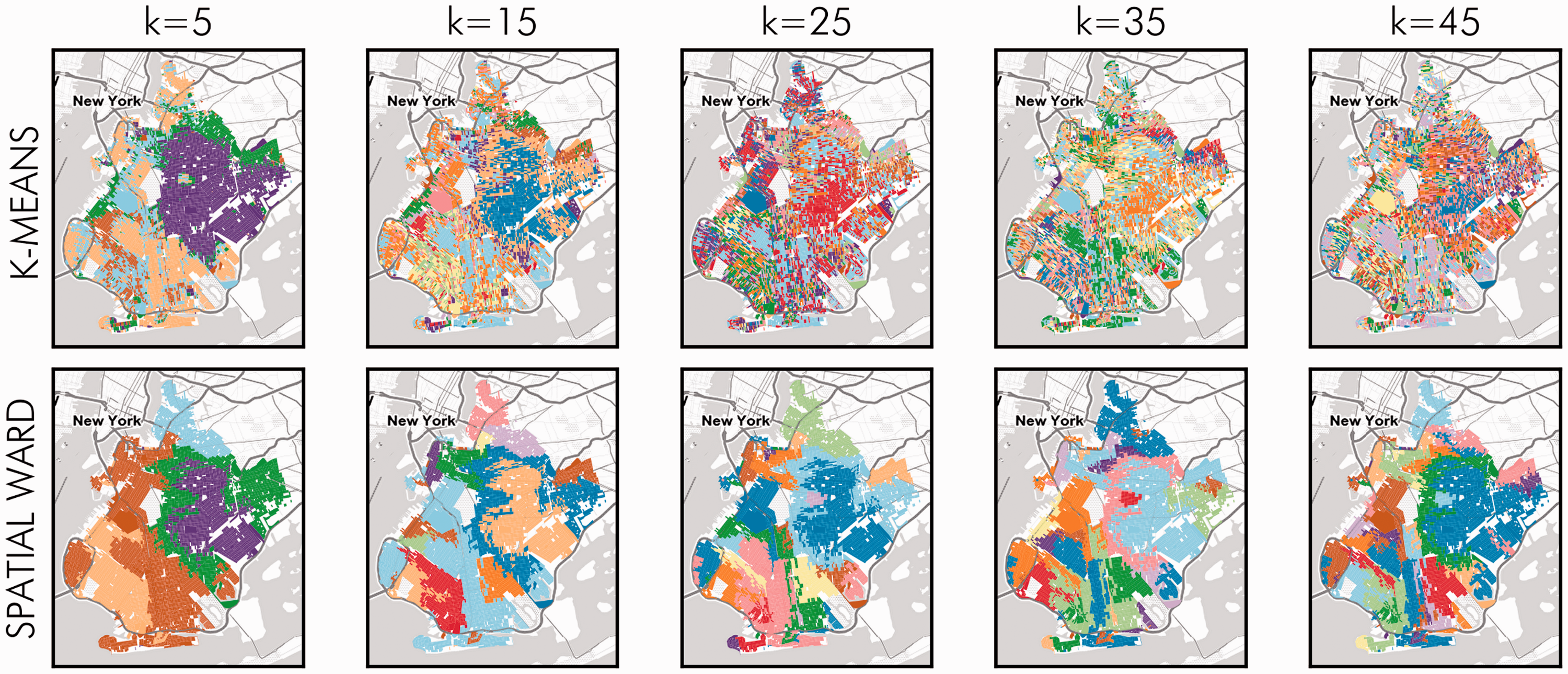
Demographic clusters in Brooklyn, NY, for k-means and spatially constrained ward agglomerative clustering. Fragmentation increases dramatically as the number of demographic clusters increases.

Another view of this fragmentation is provided by Figure 3. In this composition plot, the share of all blocks that are interior to the cluster—those that only touch other blocks in the same cluster—is represented by the gray area. The blue fraction shows blocks that are touching their NBFC. These are blocks where the “second-best choice” assignment is feasible, since the block could be re-classified to its second-best choice and not affect the spatial fragmentation in the map. Finally, the red area denotes the share of blocks that are on the boundary of their own cluster, but are not near any member of their NBFC. These are the blocks where a “second-best choice” assignment would affect territorial integrity. In addition to the shares from latent/discovered neighborhoods, we show “empirical” fractions of the same quantities: census blocks in Zillow neighborhoods that touch a neighborhood that is next-most demographically similar to the block itself, or that are on the boundary of a neighborhood but do not touch a neighborhood that is next-most demographically similar. These are shown by the horizontal dashes crossing the right vertical axis of each facet in Figure 3.

Figure 3.

Breakdown of block types based on their boundary and next-best-fit clusters for maps shown in Figures 1 and 2. Horizontal dashes on the right side of each facet reflect the empirical percentage of boundary blocks near (or not near) that block's NBFC.

Interpreting Figure 3, we can understand a few things. First, as is mathematically necessary, the share of interior blocks declines as the number of clusters increases. Second, despite this increasing fragmentation, the number of blocks that touch their NBFC is relatively stable as the number of clusters increases. This occurs quickly for the spatial agglomerative clusters, but both are remarkably stable at around k = 20. Third, we see that groups defined without spatial information (k-means) tend to be much more fragmented than either the empirical neighborhoods or the clusters discovered using the explicit spatial clustering technique. The fraction of blocks that is interior to a cluster is consistently smaller in the aspatial k-means map, and clusters are much more dramatically interspersed. The most spatially coherent solution seen in the k-means clustering solutions (that with the smallest k) is still more fragmented than the most fragmented spatial agglomerative clustering solution (that with the largest k). Finally, the empirically observed breakdowns are quite low; given that only 7% of the 7729 blocks with non-zero population sit on the boundary between two Zillow neighborhoods, only 11% of these boundary blocks (approximately 0.08% overall) are themselves near their NBFCs. Thus, the level of spatial cohesion in the Zillow neighborhoods is much higher than even those detected using the spatially explicit clustering method.

Silhouette scores are not spatial

Focusing on the empirical case, the interplay between these NBFCs and the silhouette scores is shown in Figure 4. Note that the preponderance of silhouette scores is negative for real-world neighborhoods. This means that, in terms of their racial composition, census blocks are nearly always more similar to a different neighborhood than they are to the neighborhood in which they reside. Together, this suggests that silhouette scores will always favor more socially homogeneous neighborhoods, without regard for spatial feasibility or geographical plausibility. Neighborhoods (empirical or embedded within the data) are more diverse than these optimal socially homogeneous partitions that the silhouette refers to. Indeed, any realistic urban place geography will be considered less “well-fit” by the silhouette score, since attribute coherence and geographic coherence are usually opposing objectives. By the same logic, any spatially informed clustering method must also be less “well-fit.” Any non-geographical measure of cluster fit exhibits this same property, as noted by Shelton and Poorthuis (2019).

Figure 4.

Silhouettes and next-best-fit clusters for US Census blocks within Zillow neighborhoods in Brooklyn, NY.

Indeed, neighborhood social homogeneity should not be regarded as a necessarily intrinsically desirable normative objective when conducting place detection. Social scientists have long argued that diverse and socially integrated neighborhoods provide benefits to residents when they are able to foster meaningful social exchanges (Chaskin and Joseph, 2013; Joseph et al., 2007; Talen and Koschinsky, 2014; Tolsma and van der Meer, 2018). Further, there is evidence that neighborhood diversity in the USA is increasing, carrying important benefits for residents: methods that distill neighborhoods according to maximum demographic homogeneity may be overlooking important aspects of the ways that neighborhoods are experienced by their residents (Logan, 2013). As trends towards diversification continue, there is also recent evidence that neighborhood boundaries are perceived differently among residents from different social backgrounds (Hwang, 2016), too. Together, this suggests that neighborhood definitions are tenuous, occasionally contested, and may be defined by attribute homogeneity, resident perception, or physical demarcation—and each of these definitions has unique value in different research contexts.

Geosilhouettes: Measures of spatial cluster similarity

While silhouette scores are particularly useful for identifying spatial configurations of attribute homogeneity (such as racial and ethnic enclaves), the point we raise here is that other definitions are important and useful for other research questions; building explicitly geographic measures of fit is necessary to improve the validity of geographical work on urban regions. Therefore, contra Shelton and Poorthuis (2019), it is not the designation of a goodness of fit criterion itself that harms the construct validity of detected places; it is the inflexibility, simplicity, and arbitrariness of these criteria that makes detected regions uninteresting or unhelpful. For more interesting and helpful computational geographies, it is necessary to improve, develop, and strengthen the conceptualization and operationalization of these measures of best fit.

In short, we need better geographical measures of cluster fit. They should characterize the local attribute coherence in a way that respects or controls for spatial coherence. While others may examine Figure 2 and observe simple or straightforward fragmentation in shape (e.g. McGarigal et al., 2002), we instead take inspiration from Jacquez et al. (2008): geographical cluster fit is determined by boundaries and the social similarity of nearby observations. Fortunately, the silhouette score provides a conceptually elegant structure for this. Below, we derive two geosilhouette specifications. One, the so-called path silhouette, focuses on joint attribute-spatial affinity through the use of so-called dissimilarity paths. The other, the boundary silhouette, restricts the set of each observation’s NBFCs to only those clusters that are nearby. That is, the boundary silhouette constrains the NBFC to be a feasible cluster reassignment (Duque et al., 2011). These two methods will be derived and discussed for the three styles of clustering analyses of neighborhoods and Brooklyn census blocks.⁴

Path silhouettes

One way to make the silhouette score geographically aware is to account for the fact that objects that are closer should be rated as more similar to one another in a joint geographical–social silhouette score. Thus, let us use a dissimilarity path to model the dissimilarity between two observations, i and j, as a function of the total social dissimilarity between observations along the path connecting them. This recognizes that for i and j to be in the same geographically contiguous cluster c, they must be connected by a set of observations also in c. Thus, a “path” silhouette is a silhouette score computed using the length of dissimilarity paths from i to j as the distance metric.

From Rousseeuw (1987)’s silhouette, let us consider the N × N matrix, D, that contains every pair of distances between observations i and j. Recalling that $d_{k} (i)$ takes the ith row of D and computes the average of all j columns in cluster k, it is sufficient to modify D to account for spatial structure. For this, we will build a complement to D that expresses spatial structure. This is W, an N × N spatial affinity matrix. W may be binary, reflecting a near/not near classification common for describing adjacency in polygonal lattice data, k-nearest neighbor proximity, buffer/distance banding proximity, or a spatial kernel/basis function (Bradley et al., 2015). Regardless, W should represent symmetric spatial relationships between all pairs of observations.

Bringing D and W together, a path silhouette can be constructed on $C_{1}$ , the first-order cost matrix

C_{1} = D ○ W

(2)

where

○

denotes element-wise (Hadamard) matrix products. The shortest path from each observation to every other observation can be computed using

C_{1}

as the attribute-weighted spatial adjacency matrix, or cost matrix, to provide a complete set of dissimilarities used in a silhouette score. Let this N × N matrix of all-pairs shortest path lengths found in

C_{1}

be called C (computed using Floyd, 1962, for instance). In C, the total dissimilarity between i and j is the sum of dissimilarities along the path connecting i and j in geographic space.⁵

The path silhouette is then computed using the same formula as in equation (1), using c_ij instead of d. Since an observation’s NBFC ( ${\tilde{k}}_{i}$ ) on D alone will often not be the next-best-connected cluster in C, let us denote the next-best-connected cluster to observation i as ${\ddot{k}}_{i}$ to make it clear that ${\ddot{k}}_{i} \neq {\tilde{k}}_{i}$ in general. The path silhouette expresses the difference between the average path length from i to $j \in {\ddot{k}}_{i}$ and i to other $j \in c$ .⁶ When the path silhouette is close to 1, it indicates that i has short attribute-weighted paths to other $j \in c$ , so it is extremely close to $j \in c$ , extremely similar to $j \in c$ , or some combination thereof. Alternatively, path silhouette scores close to –1 indicate that i is much easier to connect to elements in ${\ddot{k}}_{i}$ than to other elements c; again, this can be driven by spatial and/or social factors.⁷

An example of this approach to analyzing cluster quality can be seen in Figure 5. In this color ramp, the darker purple areas are those where an observation is classed as not well fit to its cluster (since the silhouette is negative), and lighter yellow are areas where the observation is well fit. This is in the same style as Figure 4, but shows the path silhouette versions: the NBFC becomes the “next-best-connected” cluster, and the silhouettes shown are the path silhouette variant.

Figure 5.

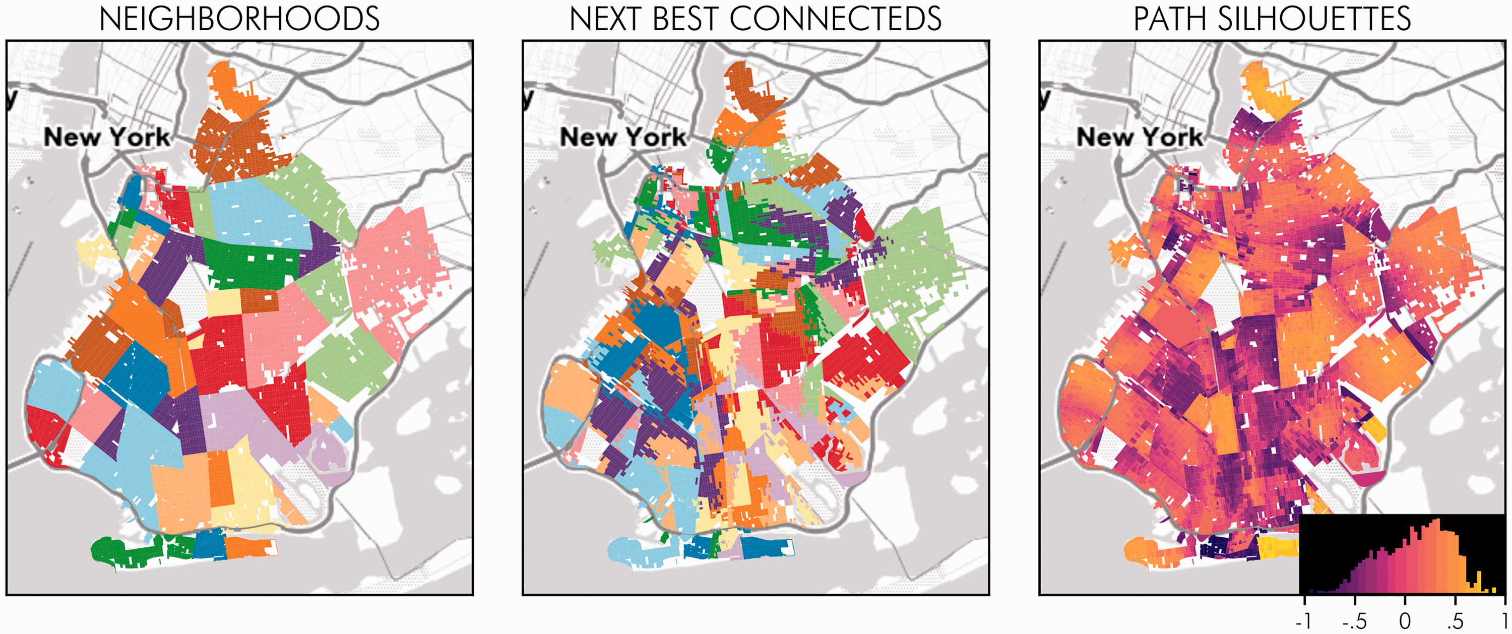
Neighborhoods and next-best-fit clusters using the path dissimilarity metric. This is the path silhouette analogue of Figure 4.

These maps show a few things. First, the geographically remote neighborhoods in the far north, west, and south of Brooklyn exhibit strong joint spatial–social cohesion due to their joint social coherence and geographical remoteness. Second (and more critically), the empirical neighborhoods with path silhouettes closer to 1 in Figure 5 tend to remain together in the spatially informed clusterings in Figure 6, even when they are in more central areas of the city. Since the path silhouette measures joint spatial–social similarity, it is reasonable that the spatial agglomerative clustering picks up on this. However, there is no constraint forcing this to occur, so this reinforces the utility of the path silhouette as an exploratory measure of the local spatial–social coherence for urban regions.

Figure 6.

Assignments to 15 clusters, silhouettes, and path silhouettes for aspatial k-means and spatial ward agglomerative clustering.

To illustrate, central Brooklyn has many neighborhoods with majority-African American populations, as shown in Figure 1. The aspatial silhouettes shown in Figure 4 show one quite clearly: East Flatbush. Recalling its atypically high silhouette scores in Figure 4 and path silhouettes in Figure 5, this area in the deep center of Brooklyn is spatially and socially distinctive. This distinctiveness is recognized regardless of cluster heuristic. In this area, both the silhouettes and the path silhouettes are high, showing this is an area with significant demographic homogeneity (a bundle of similar attributes) that is also spatially coherent (this bundle clusters geographically).

Notably, though, high path silhouettes still betray spatial–social similarity in demographically more-complex neighborhoods, such as Bushwick, along the northeast Queens–Brooklyn border. This area is not as strongly self-similar (it is not predominately mono-racial in the Census), but its profile is still distinct from other nearby neighborhoods. Path silhouettes pick up on this weaker form of spatial–social similarity, too. However, this sociogeographic distinctiveness is missed by aspatial silhouettes, regardless of the clustering heuristic. The “core” of Bushwick is assigned its own cluster in the spatial Ward clustering, and shares the same high path silhouette values as the empirical neighborhoods. Thus, geographical measures of cluster fit like the path silhouette can identify geographical exemplars: the components of a geographical cluster that are spatially and socially distinctive for that cluster.

Boundary silhouettes

While path silhouettes are a novel useful measure of joint social–spatial similarity, it too suggests a somewhat unrealistic “second-best choice” counterfactual: when computing the NBFC, the cost of moving i from c to k is modeled by the average length of paths from i to $j \in k$ . This captures both spatial and social distance. But, neighborhoods, recovered or received, are usually not point-to-point paths. While we believe these geographical data-weighted path lengths are a better model of spatial reassignment costs than nothing at all, it remains only one possible model of the actual reassignment costs, which will be different for every heuristic and clustering objective. So, we suggest a second, more conservative measure of spatial–social proximity in clusters and regions: consider only those observations that might be reassigned without affecting other observations. That is, focus on the cluster boundaries.

Consider that for each i, the NBFC ${\tilde{k}}_{i}$ is identified out of all available clusters. In the standard silhouette, ${\tilde{k}}_{i}$ has no predetermined spatial relationship to i. Often, it is geographically distant from i—indeed, the “second-choice” for i may never plausibly contain i. Whereas the path silhouette considers the cost of connecting i and all elements in other ${\tilde{k}}_{i}$ , a more conservative approach would consider only the clusters that are near i. In this way, we are constructing the best local alternative cluster for i, instead of the NBFC over the entire map.

In light of this, a boundary silhouette is defined as a restriction of the standard silhouette score. Reprising the original silhouette statement from equation (1)

s (i) = \frac{\min {{\bar{d}}_{k} (i)} - {\bar{d}}_{c} (i)}{\max {\min {{\bar{d}}_{k} (i)}, {\bar{d}}_{c} (i)}}

(3)

the boundary silhouette must restrict $\min {\bar{d}}_{k} (i)$ to only clusters where i could be reassigned without affecting any other j. So, to disqualify distant alternatives, for any k that is not geographically near i, ${\bar{d}}_{k} (i)$ is set arbitrarily high. Then, our target counterfactual “second-best choice” for i—called the best local alternative cluster—has three properties: (A) it does not contain i, (B) it is geographically near i, and (C) it has the lowest average attribute dissimilarity to i. It is helpful to denote the best local alternative as ${\hat{k}}_{i}$ , since it is often the case that ${\hat{k}}_{i} \neq {\ddot{k}}_{i} \neq {\tilde{k}}_{i}$ . In fact, depending on the notion of geography used to define local and the relative scales of the clusters and what is being clustered, there may only be one or two alternative clusters near i.⁸ It also may be true that ${\hat{k}}_{i}$ is not even a particularly good fit for i in attribute space. But, since ${\hat{k}}_{i}$ is the best cluster for which i can be reassigned without affecting other observations, it also is the best feasible second choice.

Using this idea, the boundary silhouette is the silhouette-style score between i, c, and ${\hat{k}}_{i}$ , defined only for i on the boundary. To build the set of observations on the boundary, first let us use $η (i)$ to mean the set of all observations j that are local/nearby i. Then, the set of observations on the boundary are all i for which at least one element of $η (i)$ falls in a different cluster than i’s cluster, c. This set of boundary observations is then

B = \cup_{i}^{N} {i; k_{j} \neq c \exists j \in η (i)}

(4)

Second, the set of clusters around site i can also be defined in a similar fashion

A_{i} = {k_{j}; k_{j} \neq c j \in η (i)}

(5)

Together, these definitions are sufficient to define the boundary silhouette. The “best local alternative,” the boundary silhouette’s version of the NBFC, is the cluster in $A_{i}$ that is most similar to i. With this understanding of i’s best local alternative, we can state the boundary silhouette as a familiar ratio of within- and between-cluster distances

s_{b} (i) = \frac{\min_{A_{i}} {{\bar{d}}_{k} (i)} - {\bar{d}}_{c} (i)}{\max {\min_{A_{i}} {{\bar{d}}_{k} (i)}, {\bar{d}}_{c} (i)}} \forall i \in B

(6)

This score has the same interpretation as Rousseeuw (1987)’s silhouette, but measures the cost of “flipping” i over the border of c and ${\hat{k}}_{i}$ .⁹

Practically speaking, when both sides of the boundary have a positive median boundary silhouette, it means that the parts of the clusters immediately adjacent to one another are strongly distinct. When both are negative, it suggests that the neighborhoods may be misaligned from the true underlying demographic difference in that locality. When one is positive and one is negative, the cluster on the positive side of the boundary blocks could merge with the blocks on the other side of the boundary and improve the local structure of fit without adjusting the spatial coherence of the two clusters. Thus, the boundary silhouette assesses the local goodness of fit for a cluster. It relates the similarity of the observation to its current cluster versus the cluster across the boundary.

The boundary silhouette exhibits an interesting property: it can be asymmetric for any boundary. For cluster k and cluster c, the median boundary silhouette score for observations in k bordering c may not necessarily be equal to the score for observations in c bordering k. This would imply that observations in c that are near k are more similar to observations in k, but observations in k that are near c are still closer to their own cluster, k. Put another way, assume that c has a large positive boundary silhouette and k has a large negative boundary silhouette. Then, observations in k that are geographically near c are also more demographically similar to c than they are to their currently assigned cluster, k. In reverse, observations in c that are geographically near k are more similar to their currently assigned cluster than to the i nearby alternative.

For an example, we provide an empirical illustration of the boundary silhouettes in downtown and north-central Brooklyn in Figures 7 and 8. In addition to the figures, the median boundary silhouette values for each adjacent neighborhood pair is provided in Tables 1 and 2. On the left of each plot, the neighborhoods are labeled. On the right, the boundary silhouettes are shown.

Figure 7.

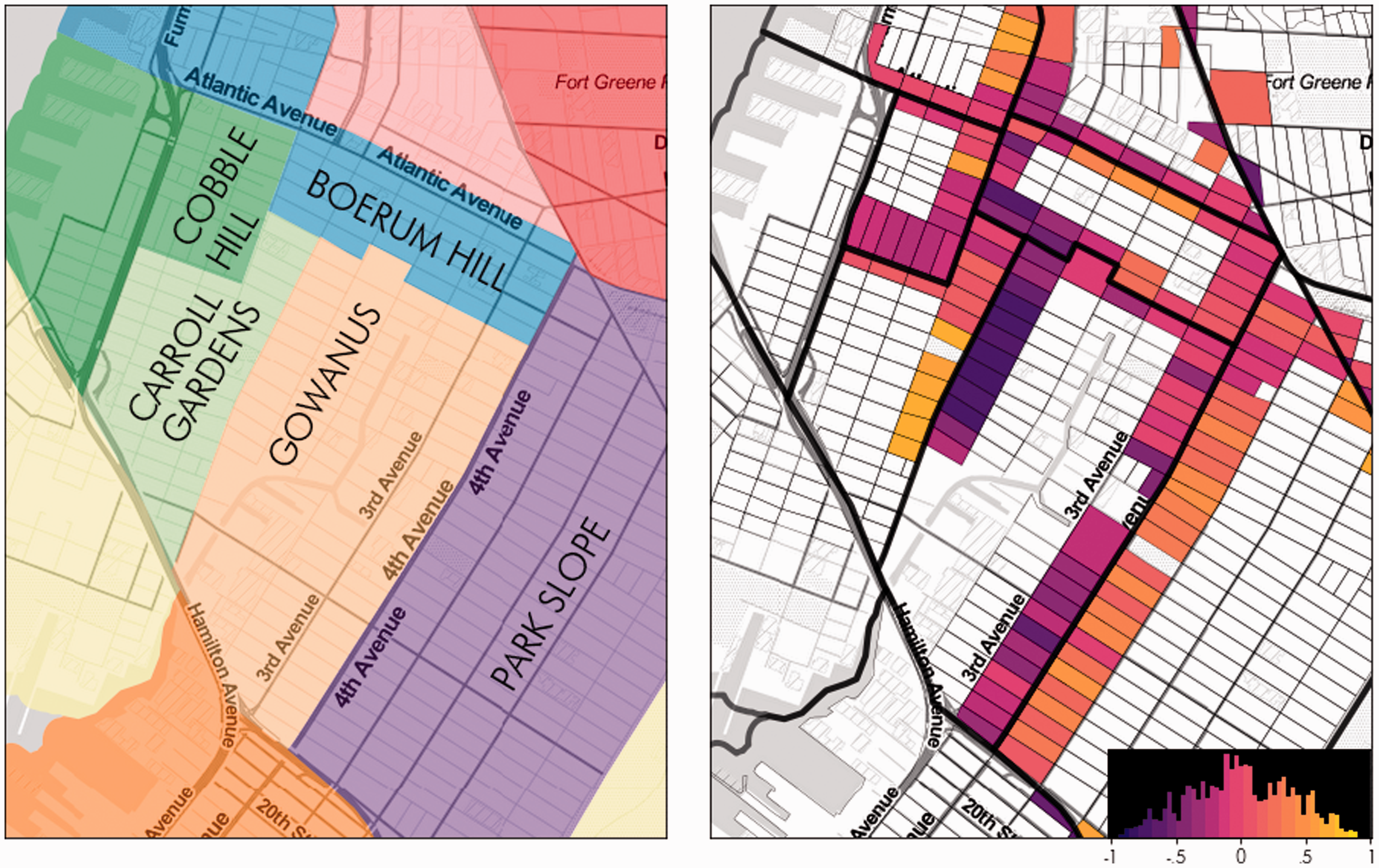
Detail of downtown Zillow neighborhoods in Brooklyn, with boundary silhouettes overlaid. The legend on the bottom right demonstrates the distribution of boundary silhouettes.

Figure 8.

Detail of north-central Zillow neighborhoods in Brooklyn, with boundary silhouettes overlaid. The legend on the bottom right demonstrates the distribution of boundary silhouettes.

Table 1.

Median boundary silhouette values for blocks abutting each cluster in downtown Brooklyn neighborhoods.

Neighbor Focal	Boerum Hill	Cobble Hill	Carroll Gardens	Gowanus	Park Slope
Boerum Hill	0.000	–0.32	–0.358	0.274	0.122
Cobble Hill	0.627	0	–0.156	0.639	–
Carroll Gardens	0.339	0.152	0	0.710	–
Gowanus	–0.071	–0.359	–0.647	0.000	–0.168
Park Slope	0.050	–	–	0.390	0

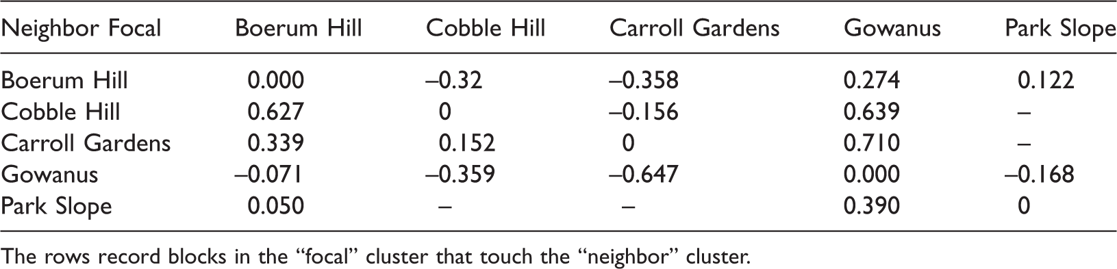
The rows record blocks in the “focal” cluster that touch the “neighbor” cluster.

Table 2.

Median boundary silhouette values for blocks abutting each cluster in north-central Brooklyn neighborhoods.

Neighbor Focal	Williamsburg	Bushwick	Bedford Stuyvesant	Clinton Hill	Crown Heights
Williamsburg	0	–0.096	0.693	0.516	–
Bushwick	0.288	0	0.482	–	–
Bedford Stuyvesant	–0.478	0.198	0.000	0.006	–0.059
Clinton Hill	–0.355	–	0.358	0	0.296
Crown Heights	–	–	0.077	–0.427	0

The rows record blocks in the “focal” cluster that touch the “neighbor” cluster.

A few strongly asymmetric boundaries are apparent. Looking at the strongest asymmetry, blocks in Gowanus near Carroll Gardens are more similar to Carroll Gardens than the rest of Gowanus, while the blocks in Carroll Gardens bordering Gowanus are much more similar to Carroll Gardens. Thus, the demographic profile of Carroll Gardens is a better demographic fit for those boundary blocks in Gowanus, so the similarity is directional, and the two neighborhoods may appear to change gradually in demographic composition when moving from Gowanus into Carroll Gardens. This contrasts with a socially undirected boundary, such as the one between Bedford-Stuyvesant and Bushwick in Figure 8. For boundaries with positive scores on both sides, social characteristics change remarkably between the boundary and its adjacent cluster. Blocks in Bushwick immediately north of Broadway Boulevard, simply could not easily be demographically passed off as a typical Bedford-Stuyvesant block.

In addition, some neighborhoods may be quite internally heterogeneous and still have positive boundary silhouettes. Plainly, a neighborhood may be an arbitrarily bounded “bundle” of inchoate and dissimilar attributes, and yet be distinct from every other bundle nearby. Some neighborhoods may even have positive and negative boundaries of nearly equal magnitude. For instance, the boundaries for Cobble Hill are positive when abutting two neighborhoods (Boerum Hill and Gowanus) but not a third (Carroll Gardens). Indeed, an even stronger example of this is in the north-central detail shown in Figure 8 with medians in Table 2. The border area between Bedford-Stuyvesant and Williamsburg is directed towards Williamsburg, but Williamsburg overall is more heterogeneous than Bedford-Stuyvesant according to their aspatial silhouette values. Further, Williamsburg blocks on the Bushwick boundary are about equally split in their demographic similarity to Williamsburg or Bushwick. This is despite the fact that Bushwick is much more demographically cohesive than Williamsburg as a whole, measured by its median aspatial silhouette score.

Discussion

Thus, between the path and boundary silhouettes, these methods introduce spatial structure into the canon of (aspatial) methods common in spatial data science. Formally, each statistic does this using a slightly different spatial structure. Both, however, introduce a formal, direct notion of geographical proximity or distance directly into the computation of social distance used to assess the coherence of a given neighborhood or the goodness of fit for an urban cluster.

The path silhouette, by mixing together attribute similarity and spatial proximity, provides a useful mechanism to measure and assess the joint spatial–social similarity in a dataset. This strategy shows increasing promise at the methodological frontiers of urban data science (Chodrow, 2017; Wolf, 2019), providing a comprehensive way to introduce an explicit model of geographical similarity into the analysis of urban clusters. The “cores” identified by path silhouettes are clustered in spatial, aspatial, and exogenously determined boundaries This shows the joint spatial–social similarity measure is useful both in empirical description and in unsupervised learning.

The boundary silhouette similarly introduces spatial thinking into a classic data science measure, but does so with a different focus in mind. Instead of specifying an explicit model for joint spatial–social similarity, this measure aims to quantify how strongly (and in which direction) does each side of a boundary align? It provides a novel, explicitly spatial method to examine how demographic differences coincide (or fail to) in the areas where regions meet. While this is a post-hoc diagnostic (rather than a boundary detection method), it can easily be incorporated into the myriad heuristics that guide cluster design, too.

It is important to note that the directional structure inherent in boundary silhouettes is not simply caused by some neighborhoods being more internally cohesive than others. These boundary silhouettes are not functions of the absolute goodness of fit of a given observation; they indicate the relative goodness of fit comparing an observation’s home cluster to its local alternatives. The aspatial silhouette also does not take into account the proximity of the next-best-fit choice; again, only 16% of blocks have their next-best-fit neighborhood as their best local alternative neighborhood. Since it is often the case that local urban structure can be quite distinct from global urban patterning (Harris, 2017; Jones et al., 2015; Leckie et al., 2012), this distinction between the relative goodness of local fit and the global best alternative considered by the classic silhouette is novel and insightful.

Conclusion

Geosilhouettes, both path and boundary variants, are immensely useful in their own right for detecting the latent social–spatial “core” of geographical regions, identifying the strength and direction of spatial boundaries, and for understanding the local socio-geographical structure of cluster fit. There is a large variety of possible refinements available for these methods, as well as possible extensions or applications. Moving forward, a classic statistical perspective could be used to identify the formal distributional properties of silhouette statistics in conditions common in urban data science (e.g. Anselin and Rey, 1991; Rey et al., 2018). Second, the strongly scale-driven reasoning embedded in the boundary silhouette could be used to generalize the analysis of boundaries between multiple levels, allowing for “local” alternatives at a micro (i.e. primitive units such as census blocks/tracks), meso (individual clusters), or macro (citywide) scale (e.g. Harris, 2017). Third, these measures could be extended to spatiotemporal clustering, applying the conceptual logic of the “second-best choice” to alternatives in time and space, or considering the trajectories of demographic classifications using a spatiotemporal distance metric (e.g. Delmelle, 2016; Delmelle et al., 2013). Fourth, a common use case of silhouettes is for graphical heuristics to identify the “optimal” number of clusters in an aspatial context; the path silhouette should provide a similar method for geographical clustering problems, and this should be further studied in future work.

At a more conceptual level, the silhouette provides a useful formal method to introduce spatial thinking because Rousseeuw (1987) is so explicit in the operationalization of their intent. Future work should be similarly explicit in intent. However, our choice to use silhouettes as the basic structure onto which geographical thinking can be grafted does not limit the scope of “spatializing” data science methods. Where possible, enhanced methods for spatial data science should make the intent of the statistic explicit and then accommodate geographical relationships directly in the statistic, rather than in post hoc geographical analysis of aspatial data science.

In our execution of this research program, we develop two new ways of measuring the local “goodness of fit” for urban clusters. Assessing the local structure of “neighborhoods,” either detected lying latent within a dataset or exogenously determined using government or colloquially defined boundaries, is a ubiquitous problem in urban data science. For the path silhouette, demographic similarity and geographical similarity are combined, providing a single measure of how cohesive neighborhoods are, both spatially and socially. For the boundary silhouette, local thinking is introduced into how observations’ are assessed for similarity. This provides an indication of how quickly or dramatically social characteristics change between two adjacent urban clusters, and speaks to the inherently multi-scale structure of urban geography.

Generally speaking, this effort participates in the broader project of developing new methods for urban spatial data science. Sometimes, is not enough to conceptualize fundamentally geographical problems in aspatial structures; instead, we suggest that introducing spatial thinking directly into the way a statistic operationalizes its core measurement is necessary to provide new insights, as we have done. Further, it is through these better concepts and operationalizations that better, more meaningful, and more useful results on the structure of urban society will be obtained.

Footnotes

Declaration of conflicting interests

The author(s) declared no potential conflicts of interest with respect to the research, authorship, and/or publication of this article.

Funding

The author(s) disclosed receipt of the following financial support for the research, authorship, and/or publication of this article: This work was supported by NSF-SES 1733705: Neighborhoods in Space-Time Contexts.

Notes

Levi J Wolf is a Senior Lecturer at the University of Bristol (UK) and a fellow with the Alan Turing Institute.

Elijah Knaap is the Assistant Director of the Center for Geospatial Sciences at the University of California, Riverside.

Sergio Rey is a Professor at the University of California, Riverside, and the founding director of the Center for Geospatial Sciences at the University of California, Riverside.

References

Anselin

Rey

(1991) Properties of tests for spatial dependence in linear regression models. Geographical Analysis 23: 112–131.

Anselin

Williams

(2016) Digital neighborhoods. Journal of Urbanism: International Research on Placemaking and Urban Sustainability 9(4): 305–328.

Arribas-Bel D and Bakens J (2018) Spatial dynamics of cultural diversity in the Netherlands. Environment and Planning B: Urban Analytics and City Science 45(6): 1142–1156.

Bradley

Wikle

Scott

(2015) Regionalization of multiscale spatial processes using a criterion for spatial aggregation error. Journal of the Royal Statistical Society 79(3): 815–832.

Chaskin

Joseph

(2013) ‘Positive’ gentrification, social control and the ‘right to the city’ in mixed-income communities: Uses and expectations of space and place. International Journal of Urban and Regional Research 37(2): 480–502.

Chodrow

(2017) Structure and information in spatial segregation. Proceedings of the National Academy of Sciences 114(44): 11591–11596.

Dean

Dong

Piekut

, et al. (2018) Frontiers in residential segregation: Understanding neighbourhood boundaries and their impacts. Tijdschrift voor economische en sociale geografie 110(3): 271–288.

Delmelle

Thill

J-C

Furuseth

, et al. (2013) Trajectories of multidimensional neighbourhood quality of life change. Urban Studies 50(5): 923–941.

Delmelle

(2016) Mapping the DNA of urban neighborhoods: Clustering longitudinal sequences of neighborhood socioeconomic change. Annals of the American Association of Geographers 106(1): 36–56.

10.

Dong

Wolf

Alexiou

, et al. (2019) Inferring neighbourhood quality with property transaction records by using a locally adaptive spatial multi-level model. Computers, Environment and Urban Systems 73: 118–125.

11.

Drukker

Kaplan

Feron

, et al. (2003) Children’s health-related quality of life, neighbourhood socio-economic deprivation and social capital. A contextual analysis. Social Science & Medicine 57(5): 825–841.

12.

Duncan

Kawachi

Subramanian

, et al. (2014) Examination of how neighborhood definition influences measurements of youths’ access to tobacco retailers: A methodological note on spatial misclassification. American Journal of Epidemiology 179(3): 373–381.

13.

Duncan

Brooks-Gunn

Klebanov

(1994) Economic deprivation and early childhood development. Child Development 65(2): 296–318.

14.

Duque

Anselin

Rey

(2012) The max-p-regions problem. Journal of Regional Science 52(3): 397–419.

15.

Duque

Church

Middleton

(2011) The P-regions problem. Geographical Analysis 43(1): 104–126.

16.

Fitzpatrick

Preisser

Porter

, et al. (2010) Ecological boundary detection using Bayesian areal wombling. Ecology 91(12): 3448–3455.

17.

Floyd

(1962) Algorithm 97: Shortest path. Communications of the ACM 5(6): 345.

18.

Fortin

M-J

Drapeau

Jacquez

(1996) Quantification of the spatial co-occurrences of ecological boundaries. Oikos 77(1): 51–60.

19.

Galster

(2001) On the nature of neighbourhood. Urban Studies 38(12): 2111.

20.

Gibbons

Nara

Appleyard

(2018) Exploring the imprint of social media networks on neighborhood community through the lens of gentrification. Environment and Planning B: Urban Analytics and City Science 45(3): 470–488.

21.

Harris

(2017) Measuring the scales of segregation: Looking at the residential separation of White British and other schoolchildren in England using a multilevel index of dissimilarity. Transactions of the Institute of British Geographers 42(3): 432–444.

22.

Harris

Sleight

Webber

(2005) Geodemographics, GIS and Neighbourhood Targeting. Vol. 7. New York: John Wiley and Sons.

23.

Hipp

Boessen

(2013) Egohoods as waves washing across the city: A new measure of “neighborhoods”. Criminology 51(2): 287–327.

24.

Hipp

Faris

Boessen

(2012) Measuring ‘neighborhood’: Constructing network neighborhoods. Social Networks 34(1): 128–140.

25.

Hwang

(2016) The social construction of a gentrifying neighborhood. Urban Affairs Review 52(1): 98–128.

26.

Isard

(1956) Regional science, the concept of region, and regional structure. Papers in Regional Science 2(1): 13–26.

27.

Jacquez

(1995) The map comparison problem: Tests for the overlap of geographic boundaries. Statistics in Medicine 14(21–22): 2343–2361.

28.

Jacquez

Kaufmann

Goovaerts

(2008) Boundaries, links and clusters: A new paradigm in spatial analysis? Environmental and Ecological Statistics 15(4): 403–419.

29.

Jacquez

Maruca

Fortin

M-J

(2000) From fields to objects: A review of geographic boundary analysis. Journal of Geographical Systems 2: 221–241.

30.

Jones

Johnston

Manley

, et al. (2015) Ethnic residential segregation: A multilevel, multigroup, multiscale approach exemplified by London in 2011. Demography 52(6): 1995–2019.

31.

Joseph

Chaskin

RJ and

Webber

(2007) The theoretical basis for addressing poverty through mixed-income development. Urban Affairs Review 42(3): 369–409.

32.

Leckie

Pillinger

Jones

, et al. (2012) Multilevel modeling of social segregation. Journal of Educational and Behavioral Statistics 37(1): 3–30.

33.

Logan

(2013) The persistence of segregation in the 21st century metropolis. City & Community 12(2): 160–168.

34.

Carlin

(2005) Bayesian areal wombling for geographical boundary analysis. Geographical Analysis 37(3): 265–285.

35.

McGarigal K, Cushman SA, Neel MC, et al. 2002 FRAGSTATS v3: Spatial Pattern Analysis Program for Categorical Maps. Computer software program produced by the authors at the University of Massachusetts, Amherst. Available at: http://www.umass.edu/landeco/research/fragstats/fragstats.html

36.

Mikelbank

(2011) Neighborhood Déjà Vu: Classification in Metropolitan Cleveland, 1970-2000. Urban Geography 32(3): 317–333.

37.

Morenoff

Sampson

Raudenbush

(2001) Neighborhood inequality, collective efficacy, and the spatial dynamics of urban violence. Criminology 39(3): 517–558.

38.

O’Campo

Xue

Wang

, et al. (1997) Neighborhood risk factors for low birthweight in Baltimore. American Journal of Public Health 87(7): 1113–1119.

39.

Pedregosa

Grisel

Blondel

, et al. (2011) Scikit-learn: Machine learning in python. Journal of Machine Learning Research 12: 2825–2830.

40.

Poorthuis

(2018) How to draw a neighborhood? The potential of big data, regionalization, and community detection for understanding the heterogeneous nature of urban neighborhoods. Geographical Analysis 50(2): 182–203.

41.

Rey

Anselin

(2007) PySAL: A Python Library of spatial analytical methods. The Review of Regional Studies 37(1): 5–27.

42.

Rey

Anselin

Folch

, et al. (2011) Measuring spatial dynamics in metropolitan areas. Economic Development Quarterly 25(1): 54.

43.

Rey

Kang

Wolf

(2018) Regional inequality dynamics, stochastic dominance, and spatial dependence. Papers in Regional Science 98(2): 861–881.

44.

Roberts

(1997) Neighborhood social environments and the distribution of low birthweight in Chicago. American Journal of Public Health 87(5): 597–603.

45.

Rousseeuw

(1987) Silhouettes: A graphical aid to the interpretation and validation of cluster analysis. Journal of Computational and Applied Mathematics 20: 53–65.

46.

Sampson

Raudenbush

Earls

(1997) Neighborhoods and violent crime: A multilevel study of collective efficacy. Science 277(5328): 918–924.

47.

Santos

Chor

Werneck

(2010) Demarcation of local neighborhoods to study relations between contextual factors and health. International Journal of Health Geographics 9(1): 1.

48.

Shelton

Poorthuis A (2019) The nature of neighborhoods: Using big data to rethink the geographies of Atlanta’s neighborhood planning unit system. Annals of the American Association of Geographers 109(5): 1341–1361.

49.

Singleton

Longley

(2009) Creating open source geodemographics: Refining a national classification of census output areas for applications in higher education. Papers in Regional Science 88(3): 643–666.

50.

Singleton

Spielman

(2014) The past, present, and future of geodemographic research in the United States and United Kingdom. The Professional Geographer 66(4): 558–567.

51.

Spielman

Folch

(2015) Reducing uncertainty in the American community survey through data-driven regionalization. PLoS One 10(2): e0115626.

52.

Spielman

Logan

(2013) Using high-resolution population data to identify neighborhoods and establish their boundaries. Annals of the Association of American Geographers 103(1): 67–84.

53.

Spielman

Yoo

E-H

Linkletter

(2013) Neighborhood contexts, health, and behavior: Understanding the role of scale and residential sorting. Environment and Planning B: Planning and Design 40(3): 489–506.

54.

Talen

Koschinsky

(2014) Compact, walkable, diverse neighborhoods: Assessing effects on residents. Housing Policy Debate 24(4): 717–750.

55.

Tolsma

van der Meer

TWG

(2018) Trust and contact in diverse neighbourhoods: An interplay of four ethnicity effects. Social Science Research 73: 92–106.

56.

Wachsmuth

Weisler

(2018) Airbnb and the rent gap: Gentrification through the sharing economy. Environment and Planning A: Economy and Space 50(6): 1147–1170.

57.

Ward

(1963) Hierarchical grouping to optimize an objective function. Journal of the American Statistical Association 58: 236–244.

58.

Wolf

(2019) Spatially-encouraged spectral clustering. Open Science Framework Preprint. Available at: https://doi.org/10.31219/osf.io/yzt2p.

59.

Womble

(1951) Differential systematics. Science 114(2961): 315–322.