Graph input representations for machine learning applications in urban network analysis

Abstract

Understanding and learning the characteristics of network paths has been of particular interest for decades and has led to several successful applications. Such analysis becomes challenging for urban networks as their size and complexity are significantly higher compared to other networks. The state-of-the-art machine learning techniques allow us to detect hidden patterns and, thus, infer the features associated with them. However, very little is known about the impact on the performance of such predictive models by the use of different input representations. In this paper, we design and evaluate six different graph input representations (i.e. representations of the network paths), by considering the network’s topological and temporal characteristics, for being used as inputs for machine learning models to learn the behavior of urban network paths. The representations are validated and then tested with a real-world taxi journeys dataset predicting the tips of using a road network of New York. Our results demonstrate that the input representations that use temporal information help the model to achieve the highest accuracy (root mean-squared error of 1.42$).

Keywords

Urban networks graph learning path representation

Introduction

Numerous important problems can be studied using the conceptual and theoretical framework of network science. Several structure and topological properties of networks have been widely studied in the recent years (Bondy, 1976; Diestel, 2005; Ferozuddin Riaz, 2011; Gross and Yellen, 2005). One of the most basic concepts in network science is the definition of network path (Ahuja, 2017; Arun and Rejimoan, 2016), i.e. a sequence of edges that joins a sequence of edges. In the case of a finite path, it is possible to identify the origin and the destination of a path as the starting and ending node of the sequence. This concept is widely used to study public infrastructures and utilities, such as trajectories and traffic flows (Kanoulas et al., 2006; Van Woensel and Vandaele, 2007), social networks (Kwak et al., 2010; Srinivasan et al., 2014), ecological networks (Dale, 2017), just to name a few. More recently, researchers have been focusing on the problem of classifying paths (Aggarwal and Wang, 2010; Jiang et al., 2016; Papa et al., 2009; Ramrez-Corona et al., 2016). For example, in the field of urban networks, classifying the paths (e.g. detecting the mean of transport) and predicting related characteristics (e.g. cost of a journey) could be useful from different perspectives. Fields of interest concern travel planning or environmental and social analysis, such as classification of urban areas, for example for understanding their wealth and wellbeing level.

Recently, machine learning (ML) techniques (Kotsiantis, 2007; Michalski et al., 1986; Murphy, 2012) have been applied to the analysis of urban networks (Duvenaud et al., 2015; Jain et al., 2016; Lee et al., 2009). However, due to memory and computational limitations, performing analysis on the networks remains challenging as their dimension increases (such as in the case of the road or transport networks of large cities). This is also due to the fact that, unlike other types of data that are easily transformed for example into time series or grids (e.g. an image can be represented as a matrix of pixels), there is no standard way of representing the network paths for using them as input to ML models. When the training dataset is large in size, ML algorithms such as random decision forests or deep neural networks require a significant amount of memory and computational power to train their models (Jordan and Mitchell, 2015; Kearns, 1989). For this reason, the traditional path representations (such as adjacency matrix) could be used only when the networks are small (their size increases exponentially with the size of the networks).

In this paper, we investigate the impact of different network path representations that can be exploited as inputs to effectively train ML models. More specifically, we designed and evaluated six different network path representations, by considering their topological and temporal characteristics, for performing ML-based classification and regression to predict characteristics associated to the paths, i.e. the value of a linked features (e.g. travel time, cost of a ride). As a proof of concept and for evaluating the proposed approach, in this paper we compute the tip of the taxi journeys using only network related features (excluding ride related information, such as cost of the ride, number of people). In particular, we consider the problem of predicting the tip of a trip by considering a real-world case study, namely the analysis of the prediction of trips contained in the New York Taxi dataset (TaxiDataset, 2018). More specifically, the prediction task that we consider is the estimation of the amount of the tip of each ride by using in input only characteristics of the road network. In particular, we compare two popular algorithms for this task, i.e. random decision forest (Ho, 1995) and deep neural networks (Bengio et al., 2013; Schmidhuber, 2015).

The key contributions of this paper can be summarized as follows:

We propose six methods, suitable for large-scale urban networks, to efficiently represent large-network paths to be used as inputs for ML algorithms. Each method is characterized by a different level of path compression and type of feature selection (e.g. preserving time and topological features).

We demonstrate that the input representations, used as input to train random decision forests and deep neural networks, are effective in classifying paths according to some shared properties (e.g. paths with similar cost or tip value). We evaluate the effectiveness of these representations by considering a real-world taxi trip dataset.

Our results show that the ML model’s performance exploiting different input representations varies according to the characteristics of the paths, such as the part of the network (i.e. neighborhoods) they cross or the importance of the origin and destination points (e.g. a node close to an airport is generally more important). For example, when the path characteristic we want to predict is simple (e.g. the distance of two points in a path), even a basic representation (e.g. a list of nodes) performs well. On the other hand, in more complex scenarios, considering the specific information about origin and destination nodes and the network topology (e.g. neighbor nodes) is fundamental to achieve high prediction accuracy. Moreover, the results of the experiments with the New York Taxi dataset demonstrate that the value of tips could be predicted with high accuracy (root mean-squared error (RMSE) 1.42$). We also observe that, for this analysis, the input representations that exploit the network topology are more effective compared to the representations that use the temporal information.

Designing graph input representations

Representation of a path

In this section we discuss the design of the path representations I (i.e. journeys in the city, public transport lines, traffic flows) that, associated to a variable y (e.g. price, time), can be used for training ML models. The ML models can then be used to predict the output variable y of new paths.

All the proposed input designs rely on a basic representation of the nodes’ position: the node vectors. A node vector in a network of N nodes is defined as an ordered list of size N, where each position in the vector corresponds to a specific node in the graph. To represent a path in a node vector, we set elements of this vector corresponding to nodes in the path as 1 (i.e. activated nodes) and the rest of the vector elements are set as 0 (i.e. not activated nodes). Consequently, for any input representation of a network path, a node vector will have at least two nodes set to 1 (i.e. origin and destination nodes in the case of a path of length 2). In urban networks, paths can represent journeys in the city, public transport lines, traffic flows, and so on.

The simplest representation of a network path is with only one node vector containing all the nodes of the path. Overall, we focus on designing graph input representations that are capable of compressing the size of paths while preserving the temporal, geographic, and semantics information. In order to further reduce the dimensionality of the input, we design representations that take into consideration only the most informative parts of a path (e.g. in paths where origin and destination points are semantically relevant places, the rest of the path may be discarded without information loss) and the topology of the network.

As shown in Figure 1, different representations can compress the paths in different ways, preserving different types of relevant information. For example, the origin and destination representation uses only origin and destination points, highlighting possible relationships between the paths and the semantics of the places; the static path representation compresses all the information in a single vector, but it does not contain any other specific information; the temporal sub-paths representation divides the static path in an ordered sequence of sub-paths; the three-steps path representation is focused on the semantic of the places and on the temporal sequence of the nodes; the k-neighbors representations (1-neighbor (d) and 2-neighbors (f) in Figure 1) consider mainly the geographic information, extending the representation to the surrounding area of the origin and destination of the paths. Finally, the three-steps k-neighbors representation merges the three-steps path and the k-neighbors representations.

Figure 1.

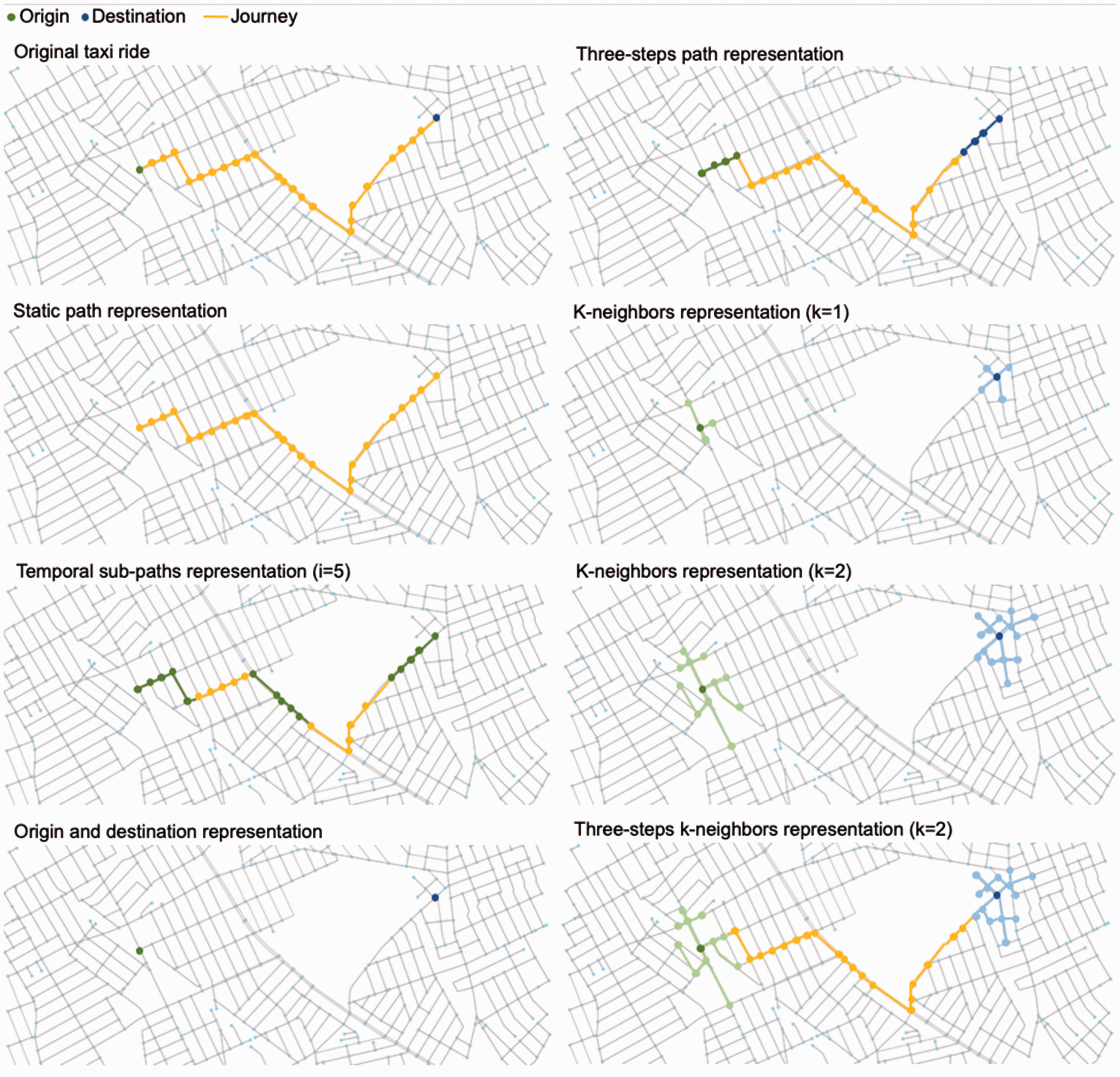
Urban network path representations for ML, each representation has different properties and advantages. (a) Original taxi ride, (b) three-steps path representation, (c) static path representation, (d) K-neighbors representation (k=1), (e) temporal sub-paths representation, (f) K-neighbors representation (k=2), (g) origin and destination representation, and (h) three-steps k-neighbors representation (k=2).

To improve the information available, combination of those representations is also analyzed in the following sections.

Static path representation

In the static path representation, the path representation consists of a single node vector in which each element corresponds to a node in the network. The element is set to 1 if the node belongs to the path, 0 otherwise (Figure 1(c)). More formally, given a graph $G = [V, E]$ with V as

V = [v_{0}, \dots, v_{N - 1}]

(1)

and a path P of length T (i.e. a sequence of T vertices) defined as

P = [v'_{0}, \dots, v'_{j}, \dots, v'_{T - 1}]

(2)

then, the resulting representation is the node vector I _static , which is defined as

I_{static} = [i_{v_{0}}, \dots, i_{v_{N - 1}}]

(3)

where:

$\forall j \in [0, N), i_{v_{j}} = 1$ if $v_{j} \in P, i_{v_{j}} = 0$ otherwise.

For example, given a network G with five nodes and a path $P = [v_{2}, v_{3}, v_{5}]$ composed of three nodes, the static path representation is

I_{static} = [0, 1, 1, 0, 1]

Temporal sub-paths representation

Temporality, the order of the nodes in the paths is often an important path feature. In predictive tasks where this is important, we propose this technique to include temporality. The temporal sub-paths representation embeds the temporal information of network paths by dividing each path into temporally ordered sub-paths. A sub-path is a sub-sequence of the original path, created by splitting it in ordered sub-sequences (i.e. the first i nodes in the path are assigned to the first sub-path, the second i nodes to the second one, and so on). Since a sub-path contains a sub-sequence of the original path, using the same logic of the static path representation, we convert each sub-path in a node vector by setting to 1 only the path nodes that belong to that sub-path. The final result is a list of node vectors, each one representing a part of the original path.

The lower is the number of nodes in each sub-path, the higher is the number of sub-paths required to represent a full path and thus the accuracy of the temporal information: in the extreme case of sub-paths with one element, all the temporal information is preserved. However, the higher is the number of sub-paths and the bigger is the size of the representation, consequentially increasing the training cost of the ML models (in terms of computational resources and time).

More formally, given a path p (see equation (2)), this input representation is the concatenation of S sub-paths ( $p_{s}$ ), where $s \in [0, \dots, S - 1]$ and a sub-path $p_{s}$ is an ordered sub-sequence of the original path P containing N_S nodes. More specifically, a sub-path is defined as

p_{s} = [v'_{N_{S} * s}, v'_{N_{S} * s + 1}, \dots, v'_{N_{S} * s + (N_{S} - 1)}]

(4)

where:

N_S is the number of path nodes in each sub-path.

Finally, each sub-path ( $p_{s}$ ) is converted to a node vector ( $I_{s}$ ) as

I_{s} = [i_{v_{0}}, \dots, i_{v_{N - 1}}]

(5)

where:

$\forall j \in [0, N), i_{v_{j}} = 1$ if $v_{j} \in p_{s}, i_{v_{j}} = 0$ otherwise.

It is worth noting that if N_S is not a divisor of T, the last sub-path would not contain exactly N_S nodes, instead it would comprise of the remainder ones (i.e. $T % N_{S}$ nodes).

Since one of our aims is to limit the size of the input, we set a limit on the maximum number of sub-paths. For simplicity, if a path exceeds the maximum number of sub-paths, the central ones are removed. The ratio behind this choice is that we hypothesize that the parts of the journeys with less information are the ones in the center, as opposed to the origin and destination parts that contain more semantic and geographic information.

Moreover, as also discussed earlier, we assume that the origin and destination nodes may be more relevant than other nodes, and, therefore, indicating them might be helpful for the network. For this reason, the first and last node vectors in the final input representation contain origin and destination nodes, respectively, and then followed by all the other node vectors in temporal order.

The resulting input representation is the following

I_{T C} = I_{0} ⊔ I_{S - 1} ⊔ I_{1} ⊔ \dots ⊔ I_{S - 2}

(6)

where:

S is the maximum number of sub-paths.

This input representation has always be of size $S \times N$ (i.e. the number of sub-paths multiplied with the total element in a node vector). Therefore, if a shorter path can only be grouped into less sub-paths than S, all the following node vectors are all set to 0. On the other hand, if a path has more sub-paths the central ones are removed as we need to preserve the information about origin and destination.

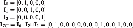
For example, given a network G with five nodes and a path $P = [v_{2}, v_{3}, v_{5}]$ composed of three nodes, the temporal sub-paths representation with S = 3 and N_S = 1 is

\begin{array}{l} I_{0} = [0, 1, 0, 0, 0] \\ I_{1} = [0, 0, 1, 0, 0] \\ I_{2} = [0, 0, 0, 0, 1] \\ I_{T C} = I_{0} ⊔ I_{2} ⊔ I_{1} = [0, 1, 0, 0, 0, 0, 0, 0, 0, 1, 0, 0, 1, 0, 0] \end{array}

Origin and destination representation

This input representation is a variant of the static path representation used when the full path is not available (e.g. enter and exit points of passengers in the underground network) and the shortest path (or any other technique to reconstruct the path) does not accurately reflect the condition of the actual path.

This representation is composed of two node vectors, one for the origin and one for the destination node of a network path (Figure 1(g)). Compared to the temporal sub-paths representation, this representation has a significantly smaller size (it is always $2 \times N$ , one node vector for the origin and one node vector for the destination) and it can thus be used to represent in a compact manner also those paths whose origin and destination points are considerably more important than the others (semantic information). Given a path P (see equation (2)), the resulting input representation is

I_{O D} = I_{start} ⊔ I_{end}

(7)

where:

$I_{start}$ is the node vector that includes only the node v₀ (all nodes set to 0 except the origin node, set to 1).

$I_{end}$ is the node vector that includes only the node $v_{T - 1}$ (all nodes set to 0 except the destination node, set to 1).

For example, given a network G with five nodes and a path $P = [v_{2}, v_{3}, v_{5}]$ composed of three nodes, the origin and destination representation is

\begin{array}{l} I_{start} = [0, 1, 0, 0, 0] \\ I_{end} = [0, 0, 0, 0, 1] \\ I_{O D} = I_{start} ⊔ I_{end} = [0, 1, 0, 0, 0, 0, 0, 0, 0, 1] \end{array}

Three-steps path representation

This technique is an extension of the origin and destination representation that, like that one, discriminates origin and destination of the journeys (temporal information) but, in addition, it includes the full path sequence of nodes (Figure 1 (b)). It is generally less accurate than the temporal sub-paths representation, but it has a significantly smaller size and it is thus suitable for huge networks (big cities or big areas).

This representation is the concatenation of the origin and destination representation and the non-temporal representation. The resulting representation has size $3 \times N$ and it is defined as follows

I_{3 s teps} = I_{O D} ⊔ I_{static}

(8)

In the first node vector, there is only the origin node set to 1, while in the second node vector only the destination node set to 1. Finally, in the third node vector, all the elements of the path are set to 1.

For example, given a network G with five nodes and a path $P = [v_{2}, v_{3}, v_{5}]$ composed of three nodes, the three-steps path representation is

I_{3 s teps} = I_{O D} ⊔ I_{static} = [0, 1, 0, 0, 0, 0, 0, 0, 0, 1, 0, 1, 1, 0, 1]

K-neighbors representation

For some classification and regression problems, it is important to exploit the network topology and to consider areas of the network instead of single nodes (e.g. in a road network, two points on the same road are generally more similar than two points at different boundaries of the city, even if their structural properties are similar). The k-neighbors representation is an enriched version of the origin and destination representation, with focus on the neighborhood of the origin and destination (geographic information) (Figure 1(d) and (f)): given a node vector with one node activated (hereafter called “base” node), the k-neighbors nodes of this base node are also activated (set to 1) in the same vector. The k-neighbors nodes of a node are its neighbors (nodes linked to it) until grade k. For example, with k = 1 only the nodes directly connected to the “base” node are included, with k = 2 also the neighbors of the neighbors of the base node are taken into account, and so on. As one of the goals of this work is to handle large urban networks and the geographic information is related to the semantic information, in this input representation the only “base” nodes selected are the origin and destination nodes (the final representation has size $2 \times N$ ).

Formally, given a path P (see equation (2)), the k-neighbors representation is

I_{K N} = I_{k - start} ⊔ I_{k - end}

(9)

where:

$I_{k - start}$ is the node vector that includes v₀ and its k-neighbors.

$I_{k - end}$ is the node vector that includes $v_{T - 1}$ and its k-neighbors.

For example, given a network G with five nodes and a path $P = [v_{2}, v_{3}, v_{5}]$ composed of three nodes, node v₂ connected to nodes v₁, v₃, v₄ and node v₅ connected only to node v₄. The k-neighbors representation is

\begin{array}{l} I_{k - start} = [1, 1, 1, 1, 0] \\ I_{k - end} = [0, 0, 0, 1, 1] \\ I_{K N} = I_{k - start} ⊔ I_{k - end} = [1, 1, 1, 1, 0, 0, 0, 0, 1, 1] \end{array}

Three-steps K-neighbors representation

Like the three-steps path representation, this representation is a combination of the k-neighbors representation and the non-temporal representation. The aim of this representation is to consider the topology of the network (using k-neighbor), the temporal information (discriminating origin and destination), and the full path, without a significant memory consumption (the input representation has size $3 \times N$ ). The resulting representation is

I_{3 s teps - K N} = I_{K N} ⊔ I_{static}

(10)

In this representation the first node vector indicates the origin node and its k-neighbors by setting them to 1, while the second node vector indicates the destination node and its k-neighbors by setting them to 1. Finally, the third node vector indicates all the nodes of the path by setting them to 1.

I_{3 s teps - K N} = I_{K N} ⊔ I_{static} = [1, 1, 1, 1, 0, 0, 0, 0, 1, 1, 0, 1, 1, 0, 1]

Evaluation setup

In this section we discuss our approach to evaluate the proposed input representations. We start with discussing the dataset used, then the construction of prediction models and, finally, we introduce the baselines and metrics for quantifying the performance of prediction models.

NYC taxi dataset

People use taxis to travel from one part of a city to another. Along with the bill there is a tip offered to the drivers that reflects the willingness of users to pay some extra money for their trips. Although the tip depends on several factors, we hypothesize that the network topology is a key factor for determining it. Therefore, we use a dataset of taxi trips for constructing a model that can predict the tip for each trip. The key motivation for using this dataset as a case study is that it can be used to improve the pricing policy of the private companies, i.e. by detecting the areas of the city with the highest willingness to pay at different times, setting the right fares, or moving the cars in more profitable areas.

We use the yellow and green taxi trip dataset (TaxiDataset) containing the information about one million taxi trips during a period of 12 months. The trip information included in the dataset is as follows: VendorID, pick-up date and time, drop-off date and time, passenger count, trip distance, pick-up longitude, pick-up latitude, RatecodeID, store and fwd flag, drop-off longitude, drop-off latitude, payment type, fare amount, extra, mta tax, tip amount, tolls amount, improvement surcharge, total amount. However, we consider only the pick-up and drop-off locations of trips to model our problem. In this work we used the dataset of the first six months of 2016, using one million of rides in the area of Manhattan and Brooklyn. We selected these two areas in order to have a variety of business and residential areas, shopping and touristic areas, as well as an airport. The journeys used for training and validating the models are filtered so as to obtain datasets with a uniform distribution of the tips. This assures that the models are general and able to predict all possible tip values, avoiding overfitting around the most common tip values.

In this work the urban network is built using the New York City road data provided by OpenStreetMap (OSM) (OSM—New York, 2018) that is composed of 20,990 nodes. In order to create a network path for each trip, the pick-up and drop-off locations of that trip are associated to the closest node in the road network and the route of the trip is then estimated by computing the shortest path with the Dijkstra’s algorithm (Dijkstra, 1959; Mehlhorn and Sanders, 2008).

Constructing predictive models

We construct models for predicting tips with each input representation by using two ML algorithms: (i) random decision forest (Ho, 1995) and (ii) deep neural network (Bengio et al., 2013; Schmidhuber, 2015). The rationale behind using these two algorithms is to test the proposed input representations with ML algorithms with different learning techniques and peculiarities. We fine tune both models by optimizing their hyper-parameters as discussed below.

Tuning random decision forest algorithm

We tune the random decision forest algorithm by optimizing the following three hyper-parameters: (i) number of trees, (ii) max depth of the trees, and (iii) minimum number of samples required to split an internal node or to be a leaf node. This is performed through a standard tuning function of the Scikit-learn Python library (Pedregosa et al., 2011).

Tuning deep neural network algorithm

In order to tune the deep neural network models, there are two key hyper-parameters to be optimized: (i) the number of hidden layers and (ii) the number of nodes in the hidden layers. However, the process of finding the optimal values for these parameters is an intricate task; consequently, we optimized the value by exploring the number of hidden layers between 1 and 5. Moreover, the number of nodes is set as follows

n_{i} = I L_{size} / (NDR \times i)

(11)

Here, n_i indicates the number of nodes in ith layer, IL_size refers to the size of input layer, and NDR refers to node division ratio, which is optimized $\in [4, 8, 16, 32, 64]$ .

Another parameter we consider for optimization is the dropout ratio (Srivastava et al., 2014), which is used to prevent overfitting of the models. During training, random nodes are dropped, along with their connections, from the neural network generating different thinned networks. During test phase, an unthinned neural network (without dropout) is used. We performed the evaluation by using values of dropout ratio between 0 and 50% with a step of 10%.

Evaluation criteria

In order to quantify the performance of models, we compute the RMSE for the test predictions. Moreover, we use the k-fold cross validation technique for validating the models because it significantly reduces bias as most of the data are used for fitting, and also significantly reduces variance as most of the data are also being used in validation set. The folds are constructed by dividing the dataset into k-folds, using k − 1 folds to train the models and the remaining one for validation. The experiments are repeated k times, in order to use each possible combination of training and validation folds, and the average of the outcomes is used as the final result.

In order to examine a model’s performance, we compare it with two baselines: overall average tip and area average tip. The overall average tip baseline is the simplest case in which the average of the overall tips in the dataset is used as a prediction output. The area average tip baseline takes the average of tips for all rides with similar departure and destination areas and uses it as prediction output. Here, an area is defined as a circle with radius r and center in the origin or destination of the considered ride. For the taxi dataset, we selected the optimal radius r by testing different values from 0.1 to 5 kilometers (optimal r is 1 kilometer).

A case study: Predicting the tip for taxi rides

In this section we present the results for the tip predicting task for given taxi trips, using the NY Taxi Journeys dataset.¹ In a taxi ride, the quantity of tip left depends on several factors, the main ones are the travel time and distance. In this case study, we argue that there are other latent factors that influence the amount of tips. In order to investigate this, we try to predict the tips left in New York City (Manhattan and Brooklyn) using exclusively the urban network graph and representing the journey path (from the origin to the destination) through the input representations defined above. We did not include the geographic distance of a journey (i.e. the sum of the length of the edges between all traversed nodes) because this would bias the results by possibly training models that compute the total length of a path to predict the tip, which is already known to be a factor that determines it. The objective is to extract information without calculating any secondary metrics calculated from the graph (e.g. distance between origin and destination). We use this approach to design general and scalable models. As a result, the input representations can be adopted in a wide range of applications where graph learning is required.

We examine the effectiveness of these input representations for training two types of ML algorithms: random decision forest and deep neural network. We chose these two algorithms because they are among the most widely used for this kind of regression problems. Moreover, their comparison represents an interesting case of study: both models tend to be very powerful yet surprisingly uncorrelated. As such, analyzing the two approaches proves the general effectiveness of the proposed input representations. Finally, both algorithms are used to construct models by using each input representation as the input, which enables us to compare the effectiveness of individual representations for enabling a model to predicting the tip for journeys. Moreover, it is worth noting that we fine-tuned models for both ML algorithms by using the grid search approach. Furthermore, we use the k-fold cross validation approach (with k = 20) to statistically validate our results.

In Figure 2 we compare the performance of models trained using the different input representations with both random decision forest and deep neural network. We use the overall average tip (RMSE 2.54$) and area average tip (RMSE 2.21$) as baselines for prediction performance. The results demonstrate that the full path itself (i.e. non-temporal representation) achieves RMSE 1.55$. However, adding temporality to the input representation (i.e. using (i) the temporal sub-paths representation and (ii) the three-steps representation) the performance of models do not improve (i.e. RMSE of 1.61$ and 1.52$, respectively). This could be due to the fact that people going from place A to place B leave a similar tip as people going from place B to place A.

Figure 2.

Tip prediction: comparison of the input representations, random decision forest and deep neural network models are trained with all the representations and their performances are compared. RMSE: root mean-squared error.

On the other hand, when we use only origin and destination nodes of a path (i.e. origin and destination representation) the trained models do not perform better than the baselines (RMSE 2.10$). This depicts that this representation does not contain enough information for effectively learning the path behavior of huge graphs. However, we observe that by considering the network topology along with origin and destination nodes (i.e. using the k-neighbors representation), the performance of models can be improved compared to using only information about the origin and destination nodes. More specifically, our models using the k-neighbors representation with k as 10 and 15 achieve the RMSE of 1.66$ and 1.57$, respectively, which is comparable to the performance of models using the non-temporal representation. Overall, we observe that the best performance (RMSE 1.42$) is achieved by using three-steps k-neighbor representation (i.e. when we concatenate the k-neighbor representation and the non-temporal representation) for constructing the models.

For completeness, we compared our results also with models that use the distance feature, a parameter already known to be correlated to the value of a tip: these models reach an accuracy comparable to the models trained using our best input representation (RMSE approximately equal to 1.51$). It is worth noting that the main difference is that our approach is not based on engineered features.

It is worth noting that the observations regarding the performance of the input representations could be specific to this prediction task. We believe that all proposed input representations should be examined in other types of prediction tasks to validate their performance for those cases. In fact, depending on the task, the relevant information could be different and thus also the best input representation. For example, predicting the fare of trips might require more temporal information, while detecting areas where people go during leisure time might require topological information.

The impact of the DNN hyper-parameters configuration is discussed in Appendix 1 (see Supplemental Material).

Trip fare prediction

Tip prediction has been chosen as the main case study because this is a complex task that depends on many factors and it represents an exemplar application for the proposed input representations. As a comparison, in this section we discuss the input representations performance with another regression task. Using the same path representations, we trained different ML models to predict trip fares using only the road network and the trip paths. This task is usually accomplished using approaches that are computationally less expensive, as trip fares are mainly a combination of distance and time. However, we performed this analysis to prove that our approach is general and that it can be applied to different types of regression tasks, with the advantage that it can also be used for in-depth graph-based socio-economic analysis of cities.

Our results show that, similarly to the main case study, neural networks and random forests models have similar performance. As expected, the length of the path influences the final cost of a journey and representations that include the full path perform better than the baselines (overall average cost RMSE 74$, area average cost RMSE 63$): static path, temporal sub-paths, and three-steps representations obtain RMSE values between 40$ and 50$. The models trained with k-neighbors representations (RMSE around 20$), surprisingly, obtain a significant improvement compared to the full path ones. These results suggest that k-neighbors representations, having the ability to detect specific areas, identify specific places (e.g. places that can be reached only using toll roads, like airports). The best results, as in the main case study, are obtained using the models trained with three-steps k-neighbors representations (RMSE 18.5$). A summary of the results is shown in Figure 3.

Figure 3.

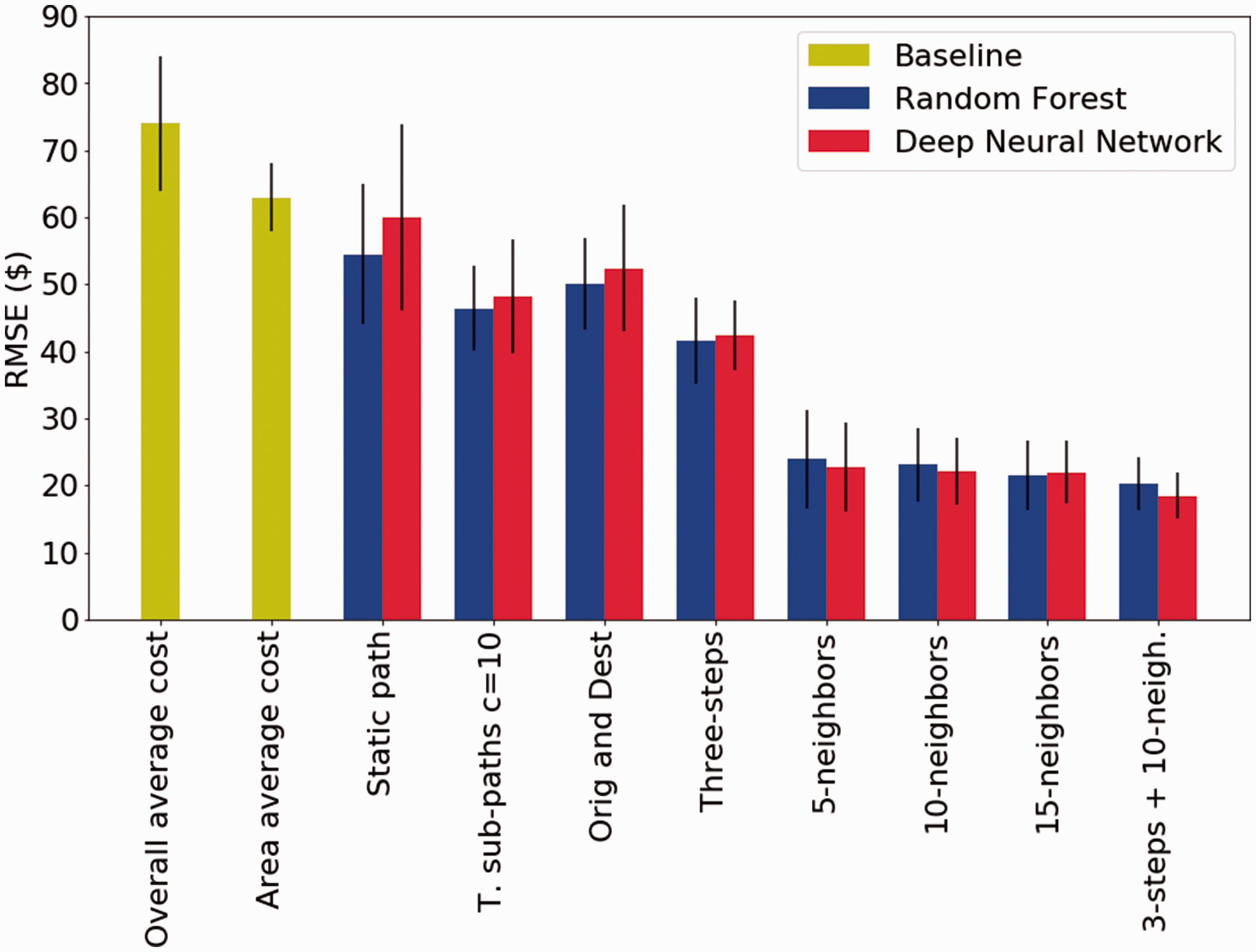
Fare prediction: comparison of the input representations, random decision forest and deep neural network models are trained with all the representations and their performances are compared. RMSE: root mean-squared error.

Performance analysis

In this section we compare the performance of the different path representations in terms of time required to train a single model and memory used. We are interested in the most computationally expensive model, i.e. deep neural networks. The graph is composed of 20,990 nodes and the models are trained on a machine with the following setup: Ubuntu 16.04, Intel Xeon CPU E5-2690 v3 2.60 GHz, 56 GB RAM, GPU Tesla K80 24 GB GDDR5.

Our analysis (Table 1) shows that the fastest representation is the static path representation (that uses only one node vector): it requires around 40 minutes to train a deep neural network model. Using two node vectors (origin and destination and k-neighbors representations) doubles the training time, while the three-steps path and three-steps k-neighbors representations (three node vectors) require, on average, 135 minutes. The most computationally intensive representations are the temporal sub-paths that, depending on the number of sub-paths, use up to 850 minutes for training a single model. From a memory usage perspective, the resource requirement has a pattern similar to time: generally, a smaller number of vector nodes requires less memory (2.4 GB for the static path representation). However, it is worth noting that, thank to software optimizations, even when the number of node vectors is the same, sparser matrices require less memory. For example, considering the k-neighbors representation, the memory required for the case of five neighbors is 4.1 GB. This raises to 5 GB for 10 neighbors and it reaches 9 GB when 15 neighbors are considered.

Table 1.

Performance comparison: time and memory required to train a single deep neural network. System used: Ubuntu 16.04, Intel Xeon CPU E5-2690 v3 2.60 GHz, 56 GB RAM, GPU Tesla K80 24 GB GDDR5.

Path representation	Time (min)	Memory (GB)
Static path	40	2.4
Temporal sub-paths (c = 5)	850	53
Temporal sub-paths (c = 10)	420	28
Origin and destination	80	2.4
Three-steps path	135	3.7
K-neighbors (k = 5)	80	4.1
K-neighbors (k = 10)	80	5
K-neighbors (k = 15)	80	9.1
Three-steps k-neighbors (k = 5)	135	5.7
Three-steps k-neighbors (k = 10)	135	6.6
Three-steps k-neighbors (k = 15)	135	10.8

Related work

In this section we review the related work in two key areas, namely the studies about design of ML techniques based on graph inputs and some examples of ML approaches already used in urban network analysis.

Graph input representations

Several graph embedding algorithms have been proposed in the past to generate vector representations for prediction tasks (Compagnon and Olliver, 2016; Cox, 1958; Grover and Leskovec, 2016; Perozzi et al., 2014). Ideally, adequate embeddings should not suffer a loss of information compared to the original graph. One of the most commonly used techniques is to obtain the decomposition of a network through clustering algorithms. For instance, one-vs-rest logistic regression (Cox, 1958) (i.e. training N different classifiers, each one designed for recognizing only a specific class) was used in relevant works such as DeepWalk (Perozzi et al., 2014) and Node2Vec (Grover and Leskovec, 2016). DeepWalk (Perozzi et al., 2014) uses local information obtained from truncated random walks to learn latent representations by treating walks as the equivalent of sentences. In Node2Vec (Grover and Leskovec, 2016), continuous feature representations are learnt for nodes in networks to map them to low-dimensional space preserving nodes neighborhoods.

Graph inputs in neural networks have been studied by Gori et al. (2005) and by Scarselli et al. (2009) as a form of recurrent neural networks. The authors use repeated application of contraction maps as propagation functions until node representations reach a stable fixed point. A propagation rule that uses convolution-like operations on graphs and methods for graph-level classification has been proposed by Duvenaud et al. (2015), which requires to learn node degree-specific weight matrices which does not scale to large graphs with wide node degree distributions. This limitation has been overcome by Kipf and Welling (2017), as they proposed a model that uses a single weight matrix per layer and deals with varying node degrees through an appropriate normalization of the adjacency matrix. In contrast to these studies that focus on identifying general network features, in this study we focus on network paths by designing input representations that enable ML algorithms to classify them or predict values that are associated with them (i.e. cost, time).

ML and urban networks

Previous works in the area of urban network networks are focused on spatio-temporal modeling (Wang et al., 2018; Yu et al., 2018): Yu et al. (2018) proposed a deep learning framework for traffic prediction, integrating graph convolution and gated temporal convolution through convolutional blocks. Their framework captures comprehensive spatio-temporal correlations through modeling multi-scale traffic networks. Wang et al. (2018) designed a generic DNN framework, used for traffic analysis and forecasting, with focus on data that are sparse in both space and time. They proposed a feed forward multilayer perceptron with each node and each edge associated with LSTM cascades instead of weights and activation functions. The estimation of fares is indeed of great interest for efficient trip planning (Noulas, 2015). The problem of taxi fare prediction using Deep Learning approaches is studied in Rossi et al. (2019). Compared to this body of work, our focus is on the representation of the paths for training a wide range of ML models, instead of the design of specific framework. Moreover, we compress the information before the training of the models. This allows researchers to deal with larger networks that could not otherwise be analyzed.

Conclusions

In this paper, we proposed six novel path input representations of urban network paths that can be used as inputs of ML algorithms for classification and regression problems. Since urban networks are usually very large in size, we designed input representations that could compress the size of the paths while aiming at preserving as much information as possible.

We examined the effectiveness of the designed input representations considering a real-world case study. More specifically, we used these representations as inputs for random decision forest and deep neural network models to predict tips for taxi journeys in New York City using a publicly available dataset as groundtruth. Our results demonstrated that the best performance (i.e. RMSE of 1.42$) is obtained by exploiting the full path enriched with the origin and destination points of the trips and their neighborhoods (three-steps k-neighbors representation). Our analysis also shows that the proposed input representations are effective for classifying urban network paths. We observe that the three-steps k-neighbors is the best representation for predicting tips of taxi rides. However, we are also aware that, depending on the path characteristics and the size of the network, the best representations for other prediction tasks may be different.

Finally, it is worth noting that the innovation of this work is not only in the application itself, but also it is mainly methodological. The proposed input representations can be applied not only to urban networks, but also to a variety of regression and classification problems based on paths in large-scale networks.

Supplemental Material

EPB892599 Supplemental Material - Supplemental material for Graph input representations for machine learning applications in urban network analysis

Supplemental material, EPB892599 Supplemental Material for Graph input representations for machine learning applications in urban network analysis by Alessio Pagani, Abhinav Mehrotra and Mirco Musolesi in EPB: Urban Analytics and City Science

Footnotes

Author’s note

Mirco Musolesi is also affiliated with University of Bologna, Italy.

Declaration of conflicting interests

The author(s) declared no potential conflicts of interest with respect to the research, authorship, and/or publication of this article.

Funding

The author(s) disclosed receipt of the following financial support for the research, authorship, and/or publication of this article: This work was supported through the EPSRC Grants EP/L006340/1 and EP/P016278/1 at UCL and by The Alan Turing Institute under the EPSRC Grant EP/N510129/1.

ORCID iD

Alessio Pagani

Note

Supplemental material

Supplemental material for this article is available online.

Alessio Pagani is a Research Associate at The Alan Turing Institute, the UK National Institute for Data Science and Artificial Intelligence. His work focuses on complex engineering systems, helping to understand the implications of inter-dependencies within and between complex adaptive systems. His current research includes the development of new methods to improve the resilience and sustainable long-term performance of man-made complex systems, addressing large uncertainties that arise due to chain reactions. He completed his PhD in Information Technology at Politecnico di Milano which involved primary research with the design of algorithms and models for the development of innovative services in the public transport.

Abhinav Mehrotra is a Research Associate at University College London. His main areas of interest include human behavior modeling and digital health. More specifically, his current research focuses on understanding and predicting human behavior by using contextual information obtained via embedded sensors for the development of intelligent systems. He also works on projects in the digital health area, in particular on the development of techniques for predicting mental health symptoms through the analysis of mobile sensing data. He obtained his PhD in Computer Science from the University of Birmingham, UK, where he worked on intelligent mobile notification systems.

Mirco Musolesi is Full Professor of Data Science at University College London (UCL) and a Turing Fellow at the Alan Turing Institute. He is also Full Professor of Computer Science at the University of Bologna. At UCL he leads the Intelligent Social Systems Lab. He received a PhD in Computer Science from University College London and a Master in Electronic Engineering from the University of Bologna. After postdoctoral work at Dartmouth College and Cambridge, he held academic posts at St Andrews and Birmingham. The focus of the work of his lab is on design of next-generation intelligent systems mainly based on computational and mathematical models of human behaviour and social dynamics. More recently, he has been interested in designing autonomous systems, possibly with humans in the loop. He is interested in both theoretical and systems-oriented aspects of these research areas. He works at the interface of several disciplines including Ubiquitous Systems, Autonomous Systems, Machine Learning, Artificial Intelligence, and Computational Social Science.

References

Aggarwal

Wang

(2010) Managing and Mining Graph Data. New York: Springer US.

Ahuja

(2017) Network Flows: Theory, Algorithms, and Applications. London: Pearson Education.

Arun

Rejimoan

(2016) A survey on network path identification using bio inspired algorithms. In: Proceedings of 2nd international conference on Advances in Electrical, Electronics, Information, Communication and Bio-Informatics (AEEICB). Chennai, India: IEEE, pp.387–389.

Bengio

Courville

Pascal

(2013) Representation learning: A review and new perspectives. IEEE Transactions on Pattern Analysis and Machine Intelligence 35: 1798–1828.

Bondy

(1976) Graph Theory with Applications. Amsterdam: Elsevier Science Ltd.

Compagnon

Olliver

(2016) Graph embeddings for social network analysis, state of the art. Master’s Thesis, INSA Lyon, France.

Cox

(1958) The regression analysis of binary sequences. Journal of the Royal Statistical Society. Series B (Methodological) 20(2): 215–242.

Dale

(2017) Applying Graph Theory in Ecological Research. Cambridge: Cambridge University Press.

Diestel

(2005) Graph Theory (Graduate Texts in Mathematics). New York: Springer.

10.

Dijkstra

(1959) A note on two problems in connexion with graphs. Numerische Mathematik 1(1): 269–271.

11.

Duvenaud

Maclaurin

Iparraguirre

, et al. (2015) Convolutional networks on graphs for learning molecular fingerprints. In: Cortes C, Lawrence ND, Lee DD, et al. (eds) Advances in Neural Information Processing Systems 28. Red Hook, NY: Curran Associates, Inc., pp.2224–2232.

12.

Ferozuddin Riaz

(2011) Applications of graph theory in computer science. In: 3D digital imaging and modeling, international conference on. Bali, Indonesia: IEEE, pp.142–145.

13.

Gori

Monfardini

Scarselli

(2005) A new model for learning in graph domains. In: Proceedings of IEEE international joint conference on neural networks. Montreal, Que., Canada: IEEE, pp.729–734.

14.

Gross

Yellen

(2005) Graph Theory and Its Applications, Second Edition (Discrete Mathematics and Its Applications). Boca Raton, FL: Chapman & Hall/CRC.

15.

Grover

Leskovec

(2016) Node2vec: Scalable feature learning for networks. In: Proceedings of the 22nd ACM SIGKDD international conference on knowledge discovery and data mining, KDD’16. San Francisco, CA, USA: ACM, pp.855–864.

16.

(1995) Random decision forests. In: Proceedings of the third international conference on document analysis and recognition, Volume 1, ICDAR 95, pp.278–282. Washington, DC: IEEE Computer Society.

17.

Jain

Zamir

Savarese

, et al. (2016) Structural-RNN: Deep learning on spatio-temporal graphs. In: Proceedings of the IEEE conference on computer vision and pattern recognition. Las Vegas, NV, USA: IEEE, pp.5308–5317.

18.

Jiang

Cui

Beutel

, et al. (2016) Catching synchronized behaviors in large networks: A graph mining approach. ACM Transactions on Knowledge Discovery from Data 10(4): 35.

19.

Jordan

Mitchell

(2015) Machine learning: Trends, perspectives, and prospects. Science 349(6245): 255–260.

20.

Kanoulas

Xia

, et al. (2006) Finding fastest paths on a road network with speed patterns. In: The 22nd international conference on Data Engineering (ICDE’06). Atlanta, GA, USA: IEEE, pp.10–20.

21.

Kearns

(1989) The computational complexity of machine learning. PhD Thesis, Harvard University, USA.

22.

Kipf

Welling

(2017) Semi-supervised classification with graph convolutional networks. In: Proceedings of ICLR.

23.

Kotsiantis

(2007) Supervised machine learning: A review of classification techniques. In: Proceedings of the 2007 conference on emerging artificial intelligence applications in computer engineering: Real word AI systems with applications in eHealth, HCI, Information Retrieval and Pervasive Technologies. The Netherlands: ACM, IOS Press Amsterdam, pp.49–268.

24.

Kwak

Lee

Park

, et al. (2010) What is twitter, a social network or a news media? In: Proceedings of the 19th international conference on world wide web, WWW ’10. Raleigh, North Carolina, USA: ACM, pp.591–600.

25.

Lee

Tseng

Tsai

(2009) A knowledge based real-time travel time prediction system for urban network. Expert Systems with Applications 36(3): 4239–4247.

26.

Mehlhorn

Sanders

(2008) Algorithms and Data Structures: The Basic Toolbox. 1st ed. New York: Springer Publishing Company, Inc.

27.

Michalski

Carbonell

Mitchell

(eds) (1986) Machine Learning an Artificial Intelligence Approach. Vol. 2. San Francisco, CA: Morgan Kaufmann Publishers Inc.

28.

Murphy KP (2012) Machine Learning: A Probabilistic Perspective. The MIT Press.

29.

Noulas A, Salnikov V, Lambiotte R, et al. (2015) Mining open datasets for transparency in taxi transport in metropolitan environments. EPJ Data Science 4(1): 23.

30.

OSM—New York (2018) Open street map. Available at: https://www.openstreetmap.org/relation/175905 (accessed 20 August 2019).

31.

Papa

Falcão

Suzuki

CTN

(2009) Supervised pattern classification based on optimum-path Forest. International Journal of Imaging Systems and Technology 19(2): 120–131.

32.

Pedregosa

Varoquaux

Gramfort

, et al. (2011) Scikit-learn: Machine learning in python. Journal of Machine Learning Research 12: 2825–2830.

33.

Perozzi

Al-Rfou

Skiena

(2014) Deepwalk: Online learning of social representations. In: Proceedings of the 20th ACM SIGKDD international conference on knowledge discovery and data mining, KDD’14. New York, NY, USA: ACM, pp.701–710.

34.

Ramrez-Corona

Sucar

Morales

(2016) Hierarchical multilabel classification based on path evaluation. International Journal of Approximate Reasoning 68: 179–193.

35.

Rossi

Barlacchi

Bianchini

, et al. (2019) Modelling taxi drivers’ behaviour for the next destination prediction. IEEE Transactions on Intelligent Transportation Systems, 1–10.

36.

Scarselli

Gori

Tsoi

, et al. (2009) The graph neural network model. IEEE Transactions on Neural Networks, 61–80.

37.

Schmidhuber

(2015) Deep learning in neural networks: An overview. Neural Networks 61: 85–117.

38.

Srinivasan

Kumar

Gupta

, et al. (2014) Stemming the Flow of Information in a Social Network. New York: Springer.

39.

Srivastava

Hinton

Krizhevsky

, et al. (2014) Dropout: A simple way to prevent neural networks from overfitting. Journal of Machine Learning Research 15: 1929–1958.

40.

TaxiDataset (2018) Tlc trip record data, nyc taxi & limousine commission. Available at: http://www.nyc.gov/html/tlc/html/about/trip_record_data.shtml (accessed 20 August 2019).

41.

Van Woensel

Vandaele

(2007) Modeling traffic flows with queueing models: A review. Asia-Pacific Journal of Operational Research (APJOR) 24(4): 435–461.

42.

Wang

Luo

Zhang

, et al. (2018) Graph-based deep modeling and real time forecasting of sparse spatio-temporal data. In: Proceedings of KDD’18.

43.

Yin

Zhu

(2018) Spatio-temporal graph convolutional networks: A deep learning framework for traffic forecasting. In: Proceedings of JCAI’18. Stockholm, Sweden, pp.3634–3640.

Supplementary Material

Please find the following supplemental material available below.

For Open Access articles published under a Creative Commons License, all supplemental material carries the same license as the article it is associated with.

For non-Open Access articles published, all supplemental material carries a non-exclusive license, and permission requests for re-use of supplemental material or any part of supplemental material shall be sent directly to the copyright owner as specified in the copyright notice associated with the article.

0.00 MB

0.29 MB