
Abstract
To explore the relationship between the objective morphological features and subjective scenic beauty preference of landscape open space units, this study improves the research method for morphology quantification, scenic beauty preference survey and relationship analysis. Fourteen morphology factors representing the features of boundary, domain and enclosure are quantified based on the point cloud data of 35 open space units. Scenic beauty evaluation is conducted online with dynamic panoramic photos. Principal component analysis is implemented to convert 14 correlated form factors into five principal components representing morphological principle. The multiple linear regression model explains the contribution of each principal component to scenic beauty preference values, showing a significance sequence of penetration, scale, naturalness, complexity and rhythm. The first three principal components have positive impacts on scenic beauty preference, while the last two principal components are negative. This work aims to reveal the regularity of public’s scenic beauty preference for open space morphology.
Introduction
In addition to performing ecological and service functions, the creation of spaces with beautiful scenery is essential to landscape spatial design. Landscape architects and researchers have applied terms of aesthetic preference, aesthetic quality, aesthetic experience and scenic beauty to express the visual appreciation of pleasing views (Chenoweth and Gobster, 1990; Daniel, 2001; Yılmaz et al., 2018). In this paper, we use the term of scenic beauty, since ‘aesthetics’ is a much broader concept. As Shafer (1969) mentioned that ‘aesthetics’ is often interpreted to involve more than just the visual senses. Scenic beauty enjoyment is considered to be the primary design objective in some landscapes, such as parks and gardens (Robinson, 2004). It is also one of the most important goals for public environmental management (Meitner, 2004). The feeling of scenic beauty is the subjective emotional feedback to objective existence, and it is evoked by both features of the landscape and the perceptual processes (Daniel, 2001). In this sense, the multiple variables that arouse the perception of scenic beauty can be classified into subjective and objective factors (Lothian, 1999). Emotions, memories, cultural and historical significance, and spiritual values may all play a part in subjective factors (Daniel, 2001), while ecology, habitat, composition elements, physical form (morphology), textures, colours, etc. compose objective factors (Robinson, 2004). Factors can be grouped not only as subjective or objective but also as constant or inconstant and quantifiable or unquantifiable (describable) (Ode et al., 2008). Spatial morphology is considered to be objective, relatively constant and quantifiable due to its physical attributes. As the concept ‘formal aesthetic’ proposed by Lang (1984) implies, designers can influence viewers’ perceptions with the formal cues given by the designer (Lang, 1994; Yılmaz et al., 2018). Therefore, this paper will focus on the correlation between objective spatial form and subjective scenic beauty preference, taking landscape open space units in built environment as examples. The landscape open space unit refers to the space that mainly enclosed by the vertical and bottom boundary (Dee, 2004) that composed of natural materials, rather than the artificial construction (e.g. streets, buildings and walls). Besides, the landscape open spaces we studied are located in the built environment rather than the natural environment, such as city parks and gardens. Landscape open spaces in the built environment are designed with human intentions to serve the needs of outdoor activities and recreations.
With the approach of scenic beauty evaluation, spatial form quantification and relationship analysis, many studies have found a significant association between spatial form and scenic beauty preference that varies depending on spatial scale, spatial type and research purpose. ① For scenic beauty preference evaluation, the most common method is the Scenic Beauty Estimation (SBE) method proposed by Daniel and Boster (1976); this method is widely used and has proved to be effective in revealing the reaction of viewers (Arriaza et al. 2004; Clay and Daniel, 2000). Most research has used still slides or photographs as a surrogate to elicit the participant’s scenic preferences (Coburn et al., 2019; Junge et al., 2015; Meitner, 2004; Zhao et al., 2013). Panoramic photos were proved to be more valid than still slides or photographs in the research done by Meitner (2004); slides and photographs are insufficient in revealing the whole formal appearance of a space because of the restricted range of view. But limited by their display platform, most panoramic photos are still presented as static expansion images (Polat and Akay, 2015; Sevenant and Antrop, 2009). In this study, we apply the 360-degree dynamic panorama display platform to avoid the partial perspective distortion that may contradict the viewer’s experience. The evaluation consistency between using photographic media and on-site experience has been proved in many studies. Stamps (1990) concluded a correlation of 0.86 between preferences obtained in site and through photographs, with 152 environments evaluated by more than 2400 participants. Palmer and Hoffman (2001) also found a weighted average correlation of 0.80 with the survey of 470 sites collectively, which appears to support the validity of using photographic representations for scenic beauty evaluation. However, the validity of using photographic media is still controversial in some researches (Daniel and Meitner, 2001; Hull and Stewart, 1992; Scott and Canter, 1997). As Scott and Canter (1997) said: ‘the experience of space is sum total of knowledge which is gained from what people see, hear, feel, smell and taste’. The differences between the photographic media and the actual scenes are undeniable, in that the photos or panoramas are taken on fixed shooting points and cannot record the smell, sound, microclimate, etc., which may affect people’s experience. However, since the purpose of this study is to discuss the relationship between scenic beauty preferences and open space unit morphology, we believe that the panoramic photos collected at the centre of the unit can record the overall morphological appearance of that space. Thus, the SBE survey using dynamic panoramic photos in this study is reliable. ② For spatial form quantification, two methods are proposed that use information from field survey, landscape photos, orthophotos and land cover data (Ode et al., 2008). One method is based on the space morphological principal of complexity, order, rhythm, harmony, coherence, imageability, naturalness, historicity, etc. (Kaplan and Kaplan, 1989; Ode et al., 2008; Ode and Miller, 2011; Tveit et al., 2006). Some of these principles can be quantified with land cover data from FRAGESTATS or ArcGIS (De la Fuente de Val et al., 2006); these data are suitable for large-scale and regional landscapes. Nevertheless, for such a relatively small space as our research object – open space in urban parks – the quantification of formal principles is barely descriptive or categorical according to perception ratings acquired by using field survey and landscape photos (Hands and Brown, 2002; Polat and Akay, 2015). The other morphology quantification method concerns the view of spatial physical organization features (scale, height, coverage (COV), shape, enclosure, etc.). However, such studies focus mostly on the forest space, as the features of height, COV and density (DEN) are quantifiable with the data of orthophotos and land cover (Daniel and Boster, 1976; Lothian, 2007). Indeed, for landscape open space unit, without accurate 3D spatial information, the porosity feature of the boundary (Casey, 2011; Dee, 2004; Stamps, 2005), open-close of the vertical enclosure (Robinson, 2004) and shape variation of the domain are difficult to quantify. Although Stamps (2005, 2009, 2011) has already done quantitative research on features that influence spaciousness, much of the research is based on model simulation rather than real-world spatial data. Thus, the absence of proper spatial information and the complexity of spatial morphology are the reasons that the use of descriptive and categorical quantification methods involves far more than the feature quantification of small space units. ③ In relationship analysis, the research purpose determines the appropriateness of an analytical method. Some methods have made a parallel comparison between single factors and scenic beauty preference by using correlation analysis and regression analysis (Othman et al., 2015; Polat and Akay, 2015; Tveit, 2009). Except for model imitation, single factor analysis cannot control the interference of other variables, nor can it express the weighted contribution of factors. Multiple linear regression (MLR) is more suitable for revealing the significant correlations of multiple variables (Abkar et al., 2011; Sevenant and Antrop, 2009). Additionally, an improved MLR method based on principal component analysis (PCA) is implemented to reduce the negative effect of the variables’ collinearity on the results in many other landscape research areas (Ul-Saufie et al., 2013) except, in most cases, scenic beauty formation.
This article compensates for the inadequacies of previous studies on spatial form quantification by ① using point clouds as spatial morphological information source of the study area; ② developing a quantitative index system of space morphology based on spatial form organization (boundaries, enclosure and domain); and ③ processing the point cloud data with CloudCompare, Grasshopper on Rhino platform and ArcGIS to achieve index quantification. Further, we also improve scenic beauty preference evaluation and relationship analysis by ① setting up an evaluation survey website that displays dynamic panoramic pictures and ② applying a PCA-based MLR analysis. Our research aims to use this analysis to explore the relationship between multiple spatial form variables (objective appearance of space) and spatial scenic beauty preferences (subjective evaluation) and to establish a regression model based on quantification. The outcome of the study reflects the extent to which formal features contribute to creation of scenic beauty and can provide a design reference on the scenic beauty creation of open space unit.
Method
Research area and data collection
Thirty-five landscape open space units are selected from five popular public urban parks in Amsterdam, including Rembrandt park, Sarphatipark, Oosterpark, Beatrixpark and Vondelpark (Figure 1). The selected units are open space dominated by groundcover and vertically surrounded by vegetation. A few trees are distributed within some unit domains, but there are too few in any of the unit domains to form a top canopy boundary. The sample units are all located in urban parks rather than in mountain areas or aside a vast lake. And the scale of such space units is not too boundless to define, neither too small to accommodation public activities. In addition, the Current Dutch Elevation (AHN3) map is available to the public. The map data (collected since 2016) are collected by laser altimetry, which records spatial morphology in point cloud data with a precision of 0.5 m. The accuracy of point clouds makes them suitable for the form analysis of the spatial scale we studied in this paper.

Thirty-five sample units in five parks.
Spatial morphology quantification
Spatial morphology factors
Form refers to the components or parts that compose the integrated spatial structure of whole landscapes spaces (Dee, 2004). In this paper, we quantify the morphology of open space unit according to its characteristics in three aspects: boundary, enclosure and domain; the morphology is determined by 14 factors (Table 1).
Fourteen morphology factors of landscape open space unit that determine the aspects of boundary, enclosure and domain.

Boundary
The boundary is the physical framework of space construction and the enclosure of the landscape space is mainly formed by the boundary (Cheng, 2009; Higuchi, 1983). In general, the environment is formed by side (vertical) boundary, top boundary and bottom boundary, no matter they are enclosed completely or not (Yan et al., 2018). In landscape open space unit, what would be the top boundary consists of the tree canopy, which is sparsely distributed and not continuous; therefore, this space type comprises primarily the vertical boundary. The vertical boundary defines the open space in the vertical direction and is composed of vegetation material. The combination and morphological characteristics of vegetation determine the opening, porosity (solid–void) and contour fluctuation of the vertical boundary morphology (Casey, 2011; Jakobsen, 1990; Wöhrle and Wöhrle, 2017, Zlatanova et al., 2020). Thus, four factors are applied to describe the form features of the vertical boundary.
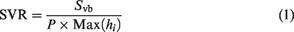
The solid–void ratio (SVR) is an indicator used to reflect the porousness feature of the landscape vertical boundary. The SVR is calculated as
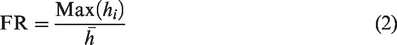
The contour fluctuation range (FR) indicates the extent of the boundary fluctuation and is defined as
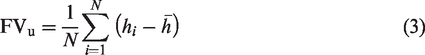
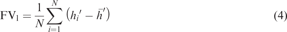
The upper contour fluctuation variance (FVu) represents the undulation intensity of the upper contour. When the value of FR is constant, the larger the FVu is, the higher the frequency at which the upper contour undulates. The FVu is calculated as
Domain
Domain suggests ownership and the territory enclosed by boundaries (Robinson, 2004). The domain of open space is the ‘void’ space that accommodates people’s activity. Many studies have already introduced area (A), visual area (VA), circularity (CIR), elongation (ELO), COV and volume density (VD) to illustrate the form features of the spatial domain (Cheng, 2009; Farina, 2008; Stamps, 2005, 2011). The difference between A and VA is that A refers to the size of domain enclosed by the vertical boundary, while VA refers to the size of area visual extends to (De la Fuente de Val et al., 2006; Dramstad et al., 2006). CIR shows the compactness and dispersion of the unit domain, which is correlated with the indexes of concavity, the area–perimeter ratio and complexity (Lin, 1998; Stamps, 2005). CIR is defined as
The ELO measures the shape extension of the unit domain. The following equation was proposed in 1969 by Webbity

The COV is defined as the percentage of the area covered by vegetation. It can be measured by assessing the portion of the ground that is covered by the existing vegetation (LEDDRiS, 2010). COV is calculated as
Moreover, VD is applied to reflect the proportion, in volume, of the domain that is occupied by vegetation (Cheng, 2009)
Enclosure
The enclosure is the comprehensive spatial experience created by the surrounding boundaries and the spatial domain. In general, the degree of enclosure on a plane is widely used to describe the limitation effect of that enclosure (Robinson, 2004). Beirão et al. (2015) proposed spaciousness as an indicator of the overall enclosure effect influenced by both the area of the vertical boundary and the area of the domain: we refer to spaciousness as the comprehensive enclosure degree (CED) in this paper. However, this vertical enclosure feature cannot fully express the enclosed state of a space; as Stamps (2005, 2009, 2013) mentioned, the impression of vertical enclosure and the perception of spaciousness are also influenced by visual permeability. Thus, we apply the concept of visual enclosure to describe the viewshed extension effect of landscape enclosure. Thus, the four factors – plane enclosure degree (PED), CED, visual extension degree (VED) and visual extension proportion (VEP) – are used to describe the enclosure feature. PED is determined by the ratio of the sum of the vertical enclosing length to the perimeter of the domain (Robinson, 2004) and is calculated as
Regarding the formula for spaciousness (Beirão et al., 2015), the CED is defined as

The VED is determined by the ratio of the visual extension area to the unit domain area and is defined as
The VEP indicates the percentage of the boundary where the viewshed extends to the unit domain perimeter length. It is calculated as
Preprocessing of point cloud data
However, not all the above indicators can be calculated directly from the point cloud data. We further transform the point cloud data into the spatial form information that is processable in a specific software (Figure 2). One is the multiple enclosure map for domain and enclosure quantification (Figure 2(a)), and the other is the boundary contour for the boundary form factor calculation (Figure 2(b)).
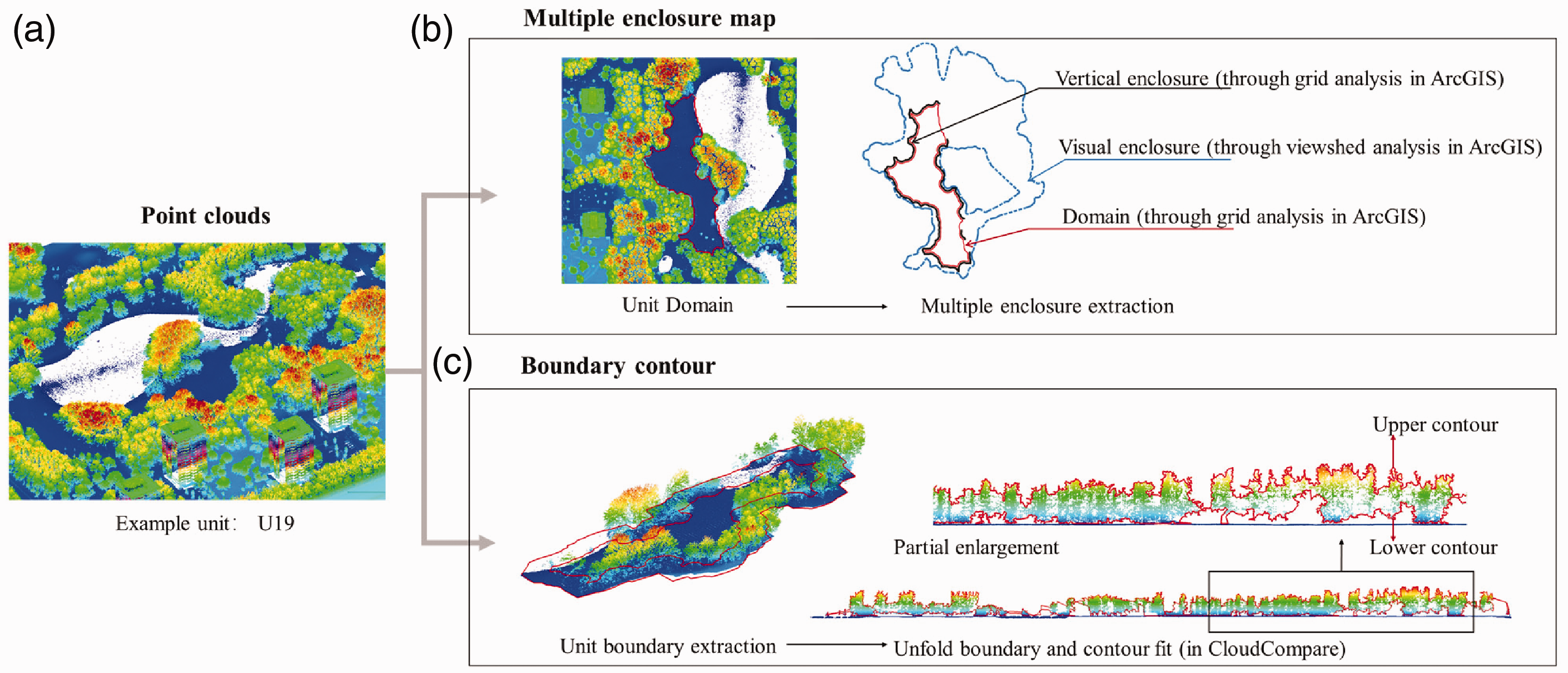
The transformation of point clouds data (take U9 as an example).
The generation of a multiple enclosure map is processed in ArcGIS, including the extraction of the unit domain, vertical enclosure and visual enclosure. The open space domain is defined as the void space surrounded by the vertical boundary and covered mainly with groundcover (Wang et al., 2020). We treat 0.3 m as the critical height for the groundcover (Booth, 1989) and as the minimum value that produces vertical restrictions. Because the AHN3 point clouds we obtained have been already classified into ground data and above-ground data, points distributed 0.3 m above the terrain are extracted and transferred to raster, where the ‘empty’ raster is the space domain dominated by the groundcover, and the ‘occupy’ raster is the vegetation-composed vertical enclosure. Furthermore, the viewshed extension range observed from observation points inside the domain is defined as the visual enclosure of that unit, which can be obtained by viewshed analysis in ArcGIS. We use solid polylines in different colours to represent the existence of the multiple enclosures: red for the unit domain, black for the vertical enclosure and blue for the visual enclosure (Figure 2(a)).
The extraction of the boundary contour is completed in CloudCompare. The buffer area with a width of 10 m outside the unit domain is clipped out for the vertical boundary morphology analysis. The Unfold and Fit tool helps to unfold the boundary contour of the unit in the format of a 2D polygon. As we can see in the example unit U9, the vertical boundary contours consist of both the upper and lower contour (Figure 2(b)), and the area between the two contours is the area of the vertical boundary.
Quantification operation
Based on the establishment of the morphological indicator system and the information obtained from point clouds, we specify an operation for each indicator and the software it can be obtained with. Among the 14 factors mentioned above, COV and VD can be calculated directly with point cloud data by CloudCompare. The values of the A and VA can be computed in ArcGIS; some basic geometry indexes that support the calculation of ELO and CIR can also be obtained in ArcGIS. For the rest factors, we build a calculation operational network for each factor in the Grasshopper plugin on the Rhino platform based on each formula (Supplemental Figure 1). The input files are the boundary contour and the multiple boundaries model we generate from point clouds. The operation network can automatically calculate the values of each factor and output the outcome in the panel by order. Calculations in Grasshopper proved to be convenient and rapid, and the morphological data of the 35 units are obtained with high efficiency.
Scenic beauty evaluation
As the scenic beauty quality is the joint product of the visible features of the landscape interacting with relevant psychological perceptions of the human observer (Daniel, 2001), the evaluation of scenic beauty should be based on the viewers’ judgement. Panoramas are taken, and serving as surrogates for mass public preference evaluation. Each panorama is obtained with 360 Panorama, since it can link several images into one panorama automatically. The panoramas of the 35 units are taken from a central position with a height of 1.6 m (general eye height of adults), thereby enabling the panoramas to reflect the overall spatial form in the viewers’ eyes (Supplemental Figure 2). To minimize the influence of climate, season and light on space appearance, the collection of the panoramas was carried out in May and completed in three days (during which the weather and climatic conditions were similar) from 10:00 to 15:00 (in similar light environments).
Compared to still photos or photo slides, panoramic photos can record the overall appearance of a space. Next, we establish a dynamic panoramic viewing website for the assessment of scenic beauty preference (link: http://pano.zhai.guru/grass1/, screen shot in Supplemental Figure 3). All the panoramas can move both vertically and horizontally, which may avoid the perspective distortion of static expansion of panoramas. The assessment of scenic beauty preference was conducted using a seven-point scale ranging from 1 = ‘very poor’ to 7 = ‘very beautiful’ (Dramstad et al., 2006; Yılmaz et al., 2018; Zhao et al., 2013). The seven-point scale is attached under each panoramic photo, and the participants are asked to rate their preference. The assessment is open to the general public. We believed that open spaces in the built environment are created for the general public, and this is the motivation of collecting public’s feedback of scenic beauty preference. The basic information of gender, age and education level are also required in the questionnaire. Followed by the SBE calculation formula proposed by Daniel and Boster (1976), the average value of the standardized rating is the final SBE value for each sample unit.
Statistical analysis
To explore the relationship between morphology data and the SBE value that we acquired by the methods mentioned above, the PCA-based MLR analysis is used in this study. PCA is carried out before MLR analysis, as too many variables and collinearity between variables may reduce the credibility of the MLR results. By using PCA, we can aggregate several collinear factors into one component that can represent the corporate effect of its constituent subfactors. Inputting 14 sets of morphology data into SPSS 25.0, PCA with a varimax rotation analysis was applied. Rotation helps to optimize the components’ structure, and only components with an eigenvalue greater than 1 are considered as principal components (PCs) (Kaiser, 1958; Ul-Saufie et al., 2013). The loading value in the rotated component matrix indicates the contribution of that factor to the PC. Taking PCs as the new independent variable and the SBE value as the dependent variable, the MLR model is created. The general equation of the model is as follows

Results
By using the procedure above, we collected all the morphology data and SBE values of the 35 spatial units (Supplemental Table 1). The distribution and standard deviation show a significant difference between units in terms of morphology features (Supplemental Table 2).
The SBE evaluation result
The scenic beauty evaluation website platform received 126 questionnaire responses. Four incomplete questionnaires were excluded; thus, 122 valid questionnaires were retained. The internal reliability coefficient (Cronbach’s alpha) of the SBE rating was 0.900, which indicates that the evaluation from 122 participants was quite reliable. The frequency of participants grouped by age shows that, 21–30 is the highest with 27.9%, followed by 31–40 and 41–50 with 22.1%, under 20 with 12.3%, 51–60 with 9.0% and lastly above 60 with 6.6%. The percentage of male respondents is 46.7% while female is 53.3%. Participants with diploma degree is held by 49.2%, high school (or under) degree by 27.9%, followed by master’s degree with 19.7% and the least is PhD with 3.2%. The correlation analysis based on groups shows that SBE ratings were not significantly correlated with gender, age or educational background (Supplemental Table 3). The SBE values of 35 units show that U25, U14, U2, U21 and U1 are the most preferred five open spaces among 35 units.
PC of spatial morphology
Since each piece of data is measured in different units, all analyses are based on normalized data. The Pearson correlation analysis result shows that 14 groups of morphological data are multiply correlated (Supplemental Table 4). Thus, PCA with varimax rotation is conducted to converge several collinear factors into one PC. The KMO and Bartlett’s test show that the data we input are sufficient for PCA (KMO = 0.563 >0.5, sig <0.01). Five PCs are extracted and account for 77.228% of the original data (Supplemental Table 5). The rotated component matrix (Table 2) clearly interprets the composition of each component and loading value (value >0.55); the larger value means that the factor is more representative of the PC.
Rotated component matrix (suppress loading value less than 0.55).
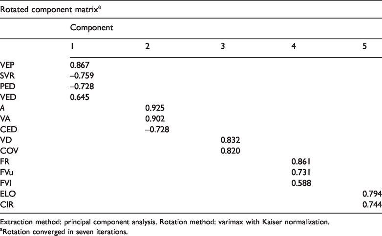
Extraction method: principal component analysis. Rotation method: varimax with Kaiser normalization.
aRotation converged in seven iterations.
Thus, 14 factors are allocated into five PCs separately. According to the constituent characteristics of each component factor, the attributes of each PC is interpreted as a morphology principle of penetration, scale, naturalness, rhythm and complexity. The details are as follows:
PC1: Penetration. The first component has a strongly positive loading on VEP (0.867) and VED (0.645), as well as a strongly negative loading on the SVR (–0.759) and the PED (–0.728). These results lead to the conclusion to illustrate PC1 as penetration, for all of these factors contribute to the penetration of spaciousness. Indeed, the incomplete vertical enclosure aggravates the infiltration characteristic; and the morphology of vegetation materials lead to the porous nature of space boundaries (Casey, 2011), creating visual penetration. PC2: Scale. The second component reflects the sense of scale since the component’s area and VA each have strong loading values (0.925 on A and 0.902 on VA). The sense of scale decreased with the increase of the CED. In the case of the same space domain area, the larger the vertical boundary forming the area is, the more constricted the space present is, which is consistent with the negative contribution of CED to PC2 (–0.728). PC3: Naturalness. DEN and vegetation COV (with values of 0.832 and 0.820, respectively) load strongly on PC3. The indicators of naturalness vary by scale in the literature, but the most common indicators are the presence and proportion of vegetation or other natural elements (Lamb and Purcell, 1990). Thus, we apply naturalness to describe the comprehensive influence of vegetation COV and DEN on the spatial unit. PC4: Rhythm. The fourth component consists of the contour FR (0.861), the FVu (0.731) and the FVl (0.588). We interpret the PC4 as ‘rhythm’, in that the three factors all represent the fluctuations of the boundary contour. PC5: Complexity. The ELO and CIR, with loading values of 0.794 and 0.744, respectively, dominate the fifth component. Both factors indicate the complexity of the spatial form.
MLR model
Taking the PCs as independent variables and the SBE as the dependent variable, two regression models are constructed by using both the enter and stepwise methods separately (Table 3). With the enter method, Model 1 takes all five PCs into account, while the stepwise-based Model 2 (which has a use probability of entry 0.05 and removal 0.2) contains only three PCs. The exclusion of naturalness (PC3) and complexity (PC5) in Model 2 indicates that these two variables have an insignificant impact on the scenic beauty of the open space unit. Comparing the two models, the discrimination coefficient value of Model 1 (R2 = 0.511) is slightly higher than that of Model 2 (R2 = 0.501), and F was determined to be 6.262 and 10.708 (F > Fa(k,n-k-1), sig<0.01). Moreover, D–W values show that no autocorrelation problems exist in either model. Thus, both models are proved to be statistically significant and convincing in explaining the relationship. Nevertheless, Model 1 is applied in this study since all the variables are included, and the R2 indicates that Model 1 has better explanation of the relationship between independents and dependent variables.
Model summary.

aPredictors: (constant), complexity, rhythm, naturalness, scale and penetration.
bPredictors: (constant), scale, penetration and rhythm.
Table 4 presents the results from enter MLR analysis between the SBE and the five PCs. The standardized coefficients (β) measure the significance of each independent PC in the regression models. Higher absolute values of β indicate a more relative importance of a PC to the SBE. Corresponding to β, the P value shows that the correlation of penetration and scale is significant at the 0.01 level (sig <0.01, two-tailed) and that the correlation of rhythm is significant at the 0.05 level (sig <0.05, two-tailed), while naturalness and complexity show low correlation. The final MLR model can be written as follows

Regression model.

aDependent variable: SBE VALUE.
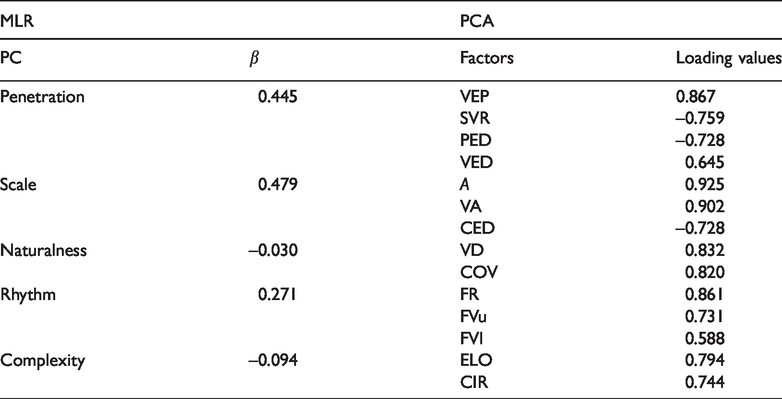
It can be concluded from the equation that the sequence of the importance of the five PCs is as follows: scale (β = 0.479), penetration (β = 0.445), rhythm (β = 0.271), complexity (β = –0.094) and naturalness (β = –0.03). The loading value represents the weight of a factor for each PC. The first three PCs have a positive impact on the creation of scenic beauty, while the two PCs with the least impact have a negative impact. Table 5 is the summary of the significance of each PC and the loading value of its composing factors.
The summary of the significance of each PC and the loading value of its composing factors.
The morphology characteristics of the top five preferred open space units (U25, U14, U2, U21 and U1) are consistent with this conclusion. The scale factors of these units present a broad sense of spatial scale. Most of the values of A and VA are close to the maximum value (max (A) = 18,178.00 and max (VA) = 56,613.30), and the rest are higher than the average (average (A) = 5770.31 and average (VA) = 16,427.22). The CED of the 35 units are distributed between 0.37 and 2.99 with an average degree of 1.09, and the CEDs of the top five preferred units are distributed between 0.44 and 0.89, presenting values that are lower than average. The data distribution of penetration also indicates a significant association. The SVR and the PED are mostly distributed over ranges lower than the average (mean (PED) = 0.81 and mean (SVR) = 0.33). Except for U14, the distribution range of VEP and VED is higher than the average range, thereby indicating a positive correlation with the SBE. Regarding the factor characteristics of rhythm, the maximum value of the FR is 2.48, and the FR of five top-rated units is between 1.85 and 2.37; these FR values can explain the positive impact of the height fluctuation on scenic beauty generation. The FVu value of the five top-rated units is almost close to the maximum (max (FVu) = 7.16), and FVl is between 2.60 and 4.31. The data regarding the CIR and ELO of each of the top five preferred units are slightly below average, thus showing a negative but relatively insignificant correlation of either of these factors with the SBE. Similarly, the factors of naturalness have a vague association with SBE, as shown by the inconsistency of data distribution range. The distribution of the data regarding the factors of naturalness with respect to these five units is lower than the average; however, U25 has a COV of 0.19 and a VD of 0.238, which are almost close to the maximum values (max (COV) = 0.2 and max (VD) = 0.27).
Discussion
The MLR model developed from the data obtained by quantifying the spatial morphology features of 35 landscape open space units reflects the characteristics of spatial scenic beauty composition and its contribution. Scale proves to be the most prominent and positive PC in open space scenic beauty creation. As Simon (2012) mentioned, the property of massiveness and comparative magnitude (or scale) may improve aesthetic qualities. The space with a wider scale is favoured by viewers (Dramstad et al., 2006). Scale being the most significant component indicates that scale is the foremost perceived spatial feature and generates positive feedback; these qualities are consistent with the cognitive process from the whole to composition. The hint of scale’s function may also result in the dominance of scale, as landscape open space unit generally accommodates public activities in urban parks, and viewers prefer space with a broader scale. However, the conclusion is based on the statistic range of 35 sample units and does not mean that the scale should be expanded infinitely for aesthetic satisfaction. The second significant PC of scenic beauty generation is penetration. This result shows that, compared to closed and introverted space, the sense of penetration produced by the boundary opening, discontinuity and porosity intensifies the scenic beauty creation of open space unit. This result is consistent with the conclusion drawn by Tveit (2009) stating that half-open space is preferred to a very closed one, since the PED of the 35 units varies from half-open (min (PED) = 0.46) to totally enclosed (max (PED) = 1). Moreover, the scenic beauty of the open space can be promoted by generating visual extension, since the visibility may evoke the imageability and gains viewers’ attention (Lynch, 1960). In addition, the result also suggests a preference of highly visible space with a half-open enclosure; this is corresponds to the prospect and refuge theory raised by Appleton (1996). Rhythm is the third main component of scenic beauty generation and is determined by the morphology of the vertical boundary. Increasing the variation range of the boundary height and strengthening the fluctuation intensity of both the upper and lower vertical boundary contours can evoke an aesthetic feeling.
However, the MLR model shows that both naturalness and complexity have an insignificant impact on landscape open space scenic beauty preference. Viewers prefer relatively aggregated and simple forms to complex domain forms. Besides, the CIR and ELO data also imply the inexistence of completely regular forms in the sample spaces; all the domain forms are irregular. Therefore, a relatively simple yet changing domain is more recommended for open space creation. Naturalness is the least negative factor among the five components; this finding is contrary to other studies (De la Fuente de Val et al., 2006; Qi et al., 2017). The reasons may include the following. ① Variations in COV and VD are not sufficiently obvious to produce scenic beauty feedback. Landscape open space consists mainly of a groundcover-dominant habitat and with a small distribution of trees; as a result, the values of COV and VD are concentrated within a small range (COV: from 0.01 to 0.20, VD: from 0.00 to 0.27). ② The limitations of the naturalness composition indicators. In this study, we take the morphology feature as the only research object, while the ecological characteristic factors relating to naturalness are not taken into account, such as level of vegetation succession (Ode et al., 2008).
This study is still limited in the following aspects. ① Boundedness morphology data interval. Some factor data obtained from the 35 units show a limited range. For example, the PED is distributed 0.46–1 since the less-enclosed space units are too vague to define. Thus, based on the collected data, this study can explain the morphology feature only within the data interval. ② Uncontrollable variables. Although we tried to control the panorama collection time and season, scenic beauty preference is also affected by other factors, such as colour, texture, roads and emotion that are uncontrollable. ③ Limitations of morphological indicators. The quantitative factors system developed in this paper describes mainly the overall morphological characteristics of the spatial unit. However, in relatively small space units, the shape of vegetation and vegetation composition will also have an impact on evaluation; such form features are not discussed in this paper. ④ Survey participant groups. In this study, we open the online evaluation survey to the public, rather than particular interest groups, such as landscape designers and managers. The potential differences among groups are part of future research.
Conclusion
This study improves landscape scenic beauty research by improving the method of data quantification, scenic beauty preference survey and data analysis. By using point clouds and a quantification method, 14 morphology factors reflecting the features of landscape unit boundary, domain and enclosure are extracted, and allocated to five uncorrelated PCs. PCA help interpret the descriptive aesthetic principles as a combination effect of several quantifiable morphology indicators. The PCA-based MLR model shows the significance and influence of each PC on scenic beauty preference in landscape open space units. The five PCs, in order of significance, are scale, penetration, rhythm, complexity and naturalness. The study results reveal the regularity of public’s scenic beauty preference for open space morphology, which can be applied to the process of landscape design and management. For landscape designers, the significance of each component and the loading value of its composing factors suggest the weightiness of space creation, and the data distribution intervals also provide reference parameters for landscape open space formation. For landscape managers, the research results can help to predict user preference, assess space quality and make decisions. Additionally, for landscape researchers, the morphology quantification and preference evaluation methods in this paper can be applied to many other types of spaces in built environment.
Supplemental Material
sj-jpg-1-epb-10.1177_2399808320949885 - Supplemental material for Exploring the relationship between spatial morphology characteristics and scenic beauty preference of landscape open space unit by using point cloud data
Supplemental material, sj-jpg-1-epb-10.1177_2399808320949885 for Exploring the relationship between spatial morphology characteristics and scenic beauty preference of landscape open space unit by using point cloud data by Yijing Wang, Sisi Zlatanova, Jinjin Yan, Ziqiao Huang and Yuning Cheng: on behalf of the GBD 2017 Italy Cardiovascular Diseases Collaborators in EPB: Urban Analytics and City Science
Supplemental Material
sj-jpg-2-epb-10.1177_2399808320949885 - Supplemental material for Exploring the relationship between spatial morphology characteristics and scenic beauty preference of landscape open space unit by using point cloud data
Supplemental material, sj-jpg-2-epb-10.1177_2399808320949885 for Exploring the relationship between spatial morphology characteristics and scenic beauty preference of landscape open space unit by using point cloud data by Yijing Wang, Sisi Zlatanova, Jinjin Yan, Ziqiao Huang and Yuning Cheng: on behalf of the GBD 2017 Italy Cardiovascular Diseases Collaborators in EPB: Urban Analytics and City Science
Supplemental Material
sj-jpg-3-epb-10.1177_2399808320949885 - Supplemental material for Exploring the relationship between spatial morphology characteristics and scenic beauty preference of landscape open space unit by using point cloud data
Supplemental material, sj-jpg-3-epb-10.1177_2399808320949885 for Exploring the relationship between spatial morphology characteristics and scenic beauty preference of landscape open space unit by using point cloud data by Yijing Wang, Sisi Zlatanova, Jinjin Yan, Ziqiao Huang and Yuning Cheng: on behalf of the GBD 2017 Italy Cardiovascular Diseases Collaborators in EPB: Urban Analytics and City Science
Supplemental Material
sj-xlsx-4-epb-10.1177_2399808320949885 - Supplemental material for Exploring the relationship between spatial morphology characteristics and scenic beauty preference of landscape open space unit by using point cloud data
Supplemental material, sj-xlsx-4-epb-10.1177_2399808320949885 for Exploring the relationship between spatial morphology characteristics and scenic beauty preference of landscape open space unit by using point cloud data by Yijing Wang, Sisi Zlatanova, Jinjin Yan, Ziqiao Huang and Yuning Cheng: on behalf of the GBD 2017 Italy Cardiovascular Diseases Collaborators in EPB: Urban Analytics and City Science
Supplemental Material
sj-pdf-5-epb-10.1177_2399808320949885 - Supplemental material for Exploring the relationship between spatial morphology characteristics and scenic beauty preference of landscape open space unit by using point cloud data
Supplemental material, sj-pdf-5-epb-10.1177_2399808320949885 for Exploring the relationship between spatial morphology characteristics and scenic beauty preference of landscape open space unit by using point cloud data by Yijing Wang, Sisi Zlatanova, Jinjin Yan, Ziqiao Huang and Yuning Cheng: on behalf of the GBD 2017 Italy Cardiovascular Diseases Collaborators in EPB: Urban Analytics and City Science
Supplemental Material
sj-xlsx-6-epb-10.1177_2399808320949885 - Supplemental material for Exploring the relationship between spatial morphology characteristics and scenic beauty preference of landscape open space unit by using point cloud data
Supplemental material, sj-xlsx-6-epb-10.1177_2399808320949885 for Exploring the relationship between spatial morphology characteristics and scenic beauty preference of landscape open space unit by using point cloud data by Yijing Wang, Sisi Zlatanova, Jinjin Yan, Ziqiao Huang and Yuning Cheng: on behalf of the GBD 2017 Italy Cardiovascular Diseases Collaborators in EPB: Urban Analytics and City Science
Supplemental Material
sj-xlsx-7-epb-10.1177_2399808320949885 - Supplemental material for Exploring the relationship between spatial morphology characteristics and scenic beauty preference of landscape open space unit by using point cloud data
Supplemental material, sj-xlsx-7-epb-10.1177_2399808320949885 for Exploring the relationship between spatial morphology characteristics and scenic beauty preference of landscape open space unit by using point cloud data by Yijing Wang, Sisi Zlatanova, Jinjin Yan, Ziqiao Huang and Yuning Cheng: on behalf of the GBD 2017 Italy Cardiovascular Diseases Collaborators in EPB: Urban Analytics and City Science
Supplemental Material
sj-pdf-8-epb-10.1177_2399808320949885 - Supplemental material for Exploring the relationship between spatial morphology characteristics and scenic beauty preference of landscape open space unit by using point cloud data
Supplemental material, sj-pdf-8-epb-10.1177_2399808320949885 for Exploring the relationship between spatial morphology characteristics and scenic beauty preference of landscape open space unit by using point cloud data by Yijing Wang, Sisi Zlatanova, Jinjin Yan, Ziqiao Huang and Yuning Cheng: on behalf of the GBD 2017 Italy Cardiovascular Diseases Collaborators in EPB: Urban Analytics and City Science
Footnotes
Declaration of conflicting interests
The author(s) declared no potential conflicts of interest with respect to the research, authorship, and/or publication of this article.
Funding
The author(s) disclosed receipt of the following financial support for the research, authorship, and/or publication of this article: This paper is supported by Foundation of China Scholarship Council (No. 201806090016) and the Research Innovation Program of Academic Degree Graduate Students in Jiangsu Province, the project name: Study on the Formation of Landscape Architecture Based on Spatial Visual Capacity (KYCX17_0162).
Supplemental material
Supplemental material for this article is available online.
References
Supplementary Material
Please find the following supplemental material available below.
For Open Access articles published under a Creative Commons License, all supplemental material carries the same license as the article it is associated with.
For non-Open Access articles published, all supplemental material carries a non-exclusive license, and permission requests for re-use of supplemental material or any part of supplemental material shall be sent directly to the copyright owner as specified in the copyright notice associated with the article.