The impact of bike network indicators on bike kilometers traveled and bike safety: A network theory approach

Abstract

There has been recent interest in the use of network analysis to quantify bike network features and their impact on biking levels and safety. However, limited bike network indicators have been evaluated. This study introduces a list of network indicators to quantify the bike network and study its effect on bike kilometers traveled and bike–vehicle crashes. Data from the city of Vancouver, Canada, are used as a case study. Full Bayesian modeling incorporating spatial effects is employed to develop Bike Kilometers Travelled (BKT) and bike–vehicle crash models. The developed BKT models show that the bike network centrality, assortativity, and weighted slope have negative associations with BKT, while the bike network directness, length, complexity and development, and connectivity have positive associations with BKT. The developed crash models show that the bike network length, centrality, assortativity, and continuity have negative associations with bike–vehicle crashes. On the other hand, the bike network complexity and development, connectivity, and linearity have positive associations with bike–vehicle crashes. The models provide insights that can be useful for planning bike networks to increase bike traffic and improve bike safety. The models also show that some changes to a bike network to increase bike traffic should be accompanied by crash risk-mitigating measures. As well, the models can be used to identify zones within a city that require safety improvements.

Keywords

Graph theory bike kilometers traveled cyclist safety GIS (geographical information systems)network graphs

Introduction

Many road authorities worldwide are promoting biking to create sustainable and livable communities and to improve public health. However, cyclists are vulnerable road users that have an elevated injury/fatality risk, which may deter road users from biking. Therefore, understanding the underlying factors that affect biking levels and bike safety is essential for promoting biking.

Previous studies showed associations between biking levels and network features (Buehler and Pucher, 2012; Dill and Carr, 2003; Marshall and Garrick, 2010; Nelson and Allen, 1997; Osama et al., 2017; Schoner and Levinson, 2014). As well, several previous studies have identified associations between bike–vehicle crashes and network indicators (Chen, 2015; Chen et al., 2012; Cho et al., 2009; Harris et al., 2011; Kaplan and Prato, 2015; Osama and Sayed, 2016; Saha et al., 2018; Siddiqui et al., 2012; Wei and Lovegrove, 2013; Yasmin and Eluru, 2016). Bike network (on-street and off-street bike lane) indicators are developed using network theory where they were found to be significantly associated with both biking levels and bike–vehicle crashes. These network indicators included connectivity, directness, and linearity. However, many other network indicators can be employed to evaluate bike networks, such as network centrality (network inter-connectivity and accessibility), assortativity (the propensity of similar nodes to be linked), complexity (network development), and robustness (the network ability to maintain its connectivity after the deletion of a node). Network indicators are useful tools for network planners, as they can be used to identify deficiencies in the network to improve safety. This is especially important when some network indicators may have contradictory associations with promoting biking and reducing bike crashes.

This paper provides a review of various bike network indicators and investigates their relationship with biking levels and safety. Full Bayesian (FB) models incorporating spatial effects are developed to assess the effect of bike network indicators (e.g. centrality, assortativity, complexity, and robustness) on Bike Kilometers Travelled (BKT) and bike–vehicle crashes. The models are developed by employing data for 134 traffic analysis zones (TAZs) in the city of Vancouver, Canada.

Previous work

Effect of bike network indicators on biking levels

Many studies have explored the relationship between bike network features and biking levels. Previous studies explored the impact of bike network length on the number of bike commuters (Buehler and Pucher, 2012; Dill and Carr, 2003; Nelson and Allen, 1997). These studies found that the higher the bike network length is, then the higher the bike commuting. Other studies found a negative association between network slope and biking levels (Dill and Carr, 2003; Hood et al., 2011; Osama et al., 2017; Winters et al., 2016).

Several studies showed the importance of bike network connectivity on affecting biking levels (Berrigan et al., 2010; Handy and Xing, 2011; Marshall and Garrick, 2010; Mekuria et al., 2012; Osama et al., 2017; Schoner and Levinson, 2014; Winters et al., 2016). Berrigan et al. (2010) analyzed spatial data from the 2001 California Health Interview Survey from two Californian counties and showed that network connectivity has a positive correlation with walking and biking levels. Schoner and Levinson (2014) used several network indicators to measure network connectivity, size, density, and directness for 74 cities in the United States. They found that network connectivity, directness, and density were positively associated with bike commuting. A summary of the various network indicators investigated and their effect on biking levels is presented in Table S1 in the online Supplementary Material.

Bike network indicators associated with bike safety

Several studies investigated the impact of network size on bike safety. On the macro level, Wei and Lovegrove (2013) showed that an increase in the bike lane length, intersection density, traffic signals, and bus stops is associated with an increase in bike–vehicle crashes. Yasmin and Eluru (2016) studied crash frequency across TAZs. After controlling for exposure measures, sociodemographic characteristics, socioeconomic characteristics, and the built environment, they found bike network length and highway length are positively correlated with bike–vehicle crashes.

Many studies have investigated the association between network connectivity and bike safety (Cho et al., 2009; Osama and Sayed, 2016; Zhang et al., 2012). At the TAZ level, Zhang et al. (2012) employed a geographically weighted regression model to explore the association between network connectivity and pedestrians’ and bike safety. They found that the increase in network connectivity is associated with an increase in pedestrian–vehicle and bike–vehicle crashes. In contrast, Siddiqui et al. (2012), Strauss et al. (2013), and Wei and Lovegrove (2013) found that density, a network connectivity metric, is positively associated with bike–vehicle crashes. Osama and Sayed (2016) found that an increase in network connectivity is associated with an increase in bike–vehicle crashes. In addition, they found that the longer the links without hindrances or discontinuities, the safer it is to cycle.

Zhang et al. (2015) investigated the effect of bike network indicators in the form of network centrality, clustering, and the average geodesic distance on non-motorists’ safety for TAZs in 321 census tracts in Alameda County, California, USA. They suggested that a highly centered network is associated with fewer non-motorist crashes, and higher clustering road networks are also associated with fewer non-motorist crashes. A summary of the various network indicators investigated and their effect on bike–vehicle crashes is presented in Table S1 in the online Supplementary Material.

Network analysis

Kansky (1963) and Rodrigue et al. (2013) introduced indices that characterized transportation network connectivity, complexity, development, and accessibility. Centrality measurements are common in urban network analysis. Previous studies showed that centrality has a strong association with vehicle movements (Jayasinghe et al., 2015; Jiang, 2009). At the TAZ level, Zhang et al. (2011) applied three centrality measures on a road network to explore the association between network quantification and street network patterns. Similarly, In Barcelona, Spain, Porta et al. (2012) employed a kernel density estimation method to examine three street centrality measures and their relationship with economic activities. De Montis et al. (2007) introduced the assortativity and rich-club coefficients to analyze interurban network characteristics using weighted network analysis. Jiang et al. (2014) calculated the assortativity and rich-club coefficients to assess the degree of correlation in urban street networks. For an air transportation network, Ponton et al. (2013) measured the network robustness by employing the average clustering coefficient. Similarly, Yao et al. (2018) employed the average clustering coefficient to evaluate the impact of street network robustness on resident commuting efficiency and the traffic flow. Many important network indicators have been employed to investigate urban streets, air transportation, or maritime networks. For bike networks, researchers investigated the effect of indicators such as connectivity, continuity, and density. However, other indicators such as network centrality, assortativity, complexity, and robustness have not been employed in bike network analysis.

Data collection

The models developed in this study are based on 134 TAZs in the city of Vancouver, Canada. Three years (2009–2013) of bike crash data have been employed. The Metro Vancouver transportation authority provided the 2013 bike network, road network, and TAZ boundaries. The Vancouver Cycling Data Model (VCDM) provides estimates of the Annual Average Daily Bike traffic. Lastly, the city of Vancouver’s open data catalog provided the contour map.

The same data set was used previously to demonstrate the importance of accounting for mediation in safety models and to develop a comprehensive zone-based index to represent both biking attractiveness and bike crash risk (Kamel et al., 2019, 2020), modeling Bike Kilometers Traveled as a function of network characteristics (Osama et al., 2017), and accounting for measurement error in traffic exposure variables (e.g. BKT) in bike–vehicle crash modeling (Kamel and Sayed, 2020). For more details on data sources, please refer to the Data sources section of the online Supplementary Material.

Variables in the analysis

Definitions of the variables that are used in the analysis and their summary statistics are presented in Table S2 in the online Supplementary Material. The variables are divided into three main categories: crashes, exposure, and bike network indicators. To calculate bike network indicators, the bike network is characterized as a set of links and nodes. The links represent the bike lanes (on-street and off-street bike lanes), while the nodes represent the intersections between network links. For this study, the network indicators are divided into seven main categories: centrality, assortativity, complexity, robustness, connectivity, directness, and topography.

Crashes and exposures

Bike–vehicle crashes are accumulated according to their locations for each TAZ. Vehicle Kilometers Travelled (VKT) and BKT are employed as traffic exposure measures. Recently, Osama and Sayed (2016) used genuine bike exposure and BKT to develop bike–vehicle crash models. BKT is developed by multiplying each segment length by the number of trips conducted on this link and then aggregating it for each TAZ. The number of trips conducted on each link was extracted from the VCDM provided by Acuere (El Esawey et al., 2015).

Centrality

Centrality recognizes the supreme nodes within a graph (Freeman, 1978). Network centrality represents network inter-connectivity and accessibility. As the “supreme” can lead to different definitions, there are different definitions for centrality. Centrality measures include degree, betweenness, closeness, and straightness centrality that could quantify how central or important each node is inside a network.

Degree centrality

The degree centrality measures to what extent a node is connected directly by other nodes (Freeman, 1978). Influential nodes have a high degree of centrality. Previous studies have employed the degree of centrality in urban network analysis (Jiang, 2009; Porta et al., 2006; Zhang et al., 2011). The degree of centrality is calculated using equation (1), where $a_{i j} = 1$ only if node $i$ and node $j$ are connected by a link, and is equal to zero otherwise, and $n$ is the number of nodes in a network

C_{i}^{D} = \frac{1}{(n - 1)} \sum_{j = 1}^{n} a_{i j}

(1)

Betweenness centrality

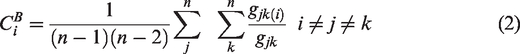
The betweenness centrality is large if the node is traversed by many of the shortest paths connecting each two nodes (Freeman, 1978), in other words, if a node is positioned between several other nodes. Several studies have used betweenness centrality in urban network analysis (Crucitti et al., 2006; Jiang, 2009; Porta et al., 2006; Zhang et al., 2011, 2015). Betweenness centrality is calculated using equation (2), where $g_{j k (i)}$ represents the number of geodesics linking nodes $j$ and $k$ that contain point $i$ on them, and $g_{j k}$ represents the number of geodesics linking nodes $j$ and $k$

C_{i}^{B} = \frac{1}{(n - 1) (n - 2)} \sum_{j}^{n} \sum_{k}^{n} \frac{g_{j k (i)}}{g_{j k}} i \neq j \neq k

(2)

Closeness centrality

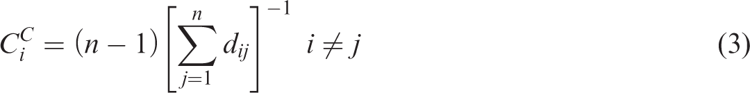
The closeness centrality is based on the notion that a node is central if a node is near to all the other nodes along the shortest paths (Freeman, 1978). It captures the travel cost of overcoming the geographic separation between nodes. Previous studies have employed closeness centrality to analyze an urban network (Crucitti et al., 2006; Jiang, 2009; Porta et al., 2006; Zhang et al., 2011). Closeness centrality is calculated using equation (3), where $d_{i j}$ represents the shortest path distance connecting nodes $i$ and $j$

C_{i}^{C} = (n - 1) {[\sum_{j = 1}^{n} d_{i j}]}^{- 1} i \neq j

(3)

Straightness centrality

The straightness centrality is based on the notion that a node is central if the paths connecting node $i$ and many other nodes are straight. Previous studies have used straightness centrality in urban network analysis (Crucitti et al., 2006; Porta et al., 2012). Straightness centrality is calculated using equation (4), where $d_{i j}^{Eucl}$ represents Euclidian distance connecting nodes $i$ and $j$

C_{i}^{S} = \frac{1}{n - 1} \sum_{i = 1}^{n} \frac{d_{i j}^{Eucl}}{d_{i j}} i \neq j

(4)

Graph centrality

Graph centrality ${(C}^{X})$ is based on node centrality. It indicates the magnitude to which the centrality of the most central point surpasses the centrality of the rest of the points, and it is a ratio to the maximum possible central graph with the same number of nodes (Freeman, 1978). Graph centrality is calculated using equation (5), where $C_{i}^{X}$ is a node centrality, and $C_{i^{*}}^{X}$ is the largest value of $C_{i}^{X}$

C^{X} = \frac{\sum_{i = 1}^{n} [C_{i^{*}}^{X} - C_{i}^{X}]}{\max \sum_{i = 1}^{n} [C_{i^{*}}^{X} - C_{i}^{X}]}

(5)

The bike network with heat maps for betweenness, straightness, closeness, and degree graph centralities for different TAZs are shown in Figure S1 in the online Supplementary Material.

Network assortativity

Assortativity is defined as the propensity of similar nodes to be linked (Newman, 2002). In this study, two metrics are proposed to quantify the network assortativity: assortativity and rich-club coefficients.

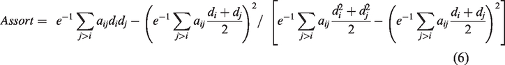
Newman (2002, 2003) suggested a concept like the Pearson correlation coefficient to quantify the assortativity coefficient. The assortativity coefficient is calculated using equation (6), where $e$ is the number of edges, $d_{i}$ and $d_{j}$ are the degrees of nodes $i$ and $j$ , $a_{i j} = 1$ if nodes $i$ and $j$ are linked to each other, $a_{i j} = 0$ otherwise (Jiang et al., 2014). $Assort > 0$ means that a network is assortative mixing, while $Assort < 0$ means it is disassortative mixing. It is calculated as follows

Assort = e^{- 1} \sum_{j > i} a_{i j} d_{i} d_{j} - {(e^{- 1} \sum_{j > i} a_{i j} \frac{d_{i} + d_{j}}{2})}^{2} / [e^{- 1} \sum_{j > i} a_{i j} \frac{d_{i}^{2} + d_{j}^{2}}{2} - {(e^{- 1} \sum_{j > i} a_{i j} \frac{d_{i} + d_{j}}{2})}^{2}]

(6)

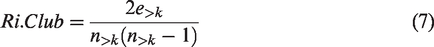
The rich-club coefficient is a specific representation of the degree correlations in a network. It focuses on the higher connectivity nodes (rich nodes). The rich-club coefficient is the proportion of the links connecting the higher connectivity nodes (rich nodes) to the possible links for the rich nodes to produce a complete graph (Jiang et al., 2014; Zhou and Mondragon, 2004). The rich-club coefficient is calculated using equation (7), where $e_{> k}$ is the number of links among the higher connectivity nodes (nodes with degrees greater than $k$ ), and $n_{> k}$ is the number of rich nodes. Few TAZs have one-degree nodes; therefore, to avoid TAZs with zero value $k$ is set equal to one. It is calculated as follows

R i . Club = \frac{2 e_{> k}}{n_{> k} (n_{> k} - 1)}

(7)

The bike network along with heat maps for assortativity and rich-club coefficients for different TAZs are shown in Figure S2 in the online Supplementary Material.

Network complexity

Rodrigue et al. (2013) introduced two network metrics to quantify network development and complexity: the Pi index and the number of cycles. The Pi index is the ratio between the network diameter and the length of the network. Rodrigue et al. (2013) defined the network diameter as “the length of the shortest path between the most distanced nodes of a network.” The number of cycles is the number of independent cycles, and it is calculated using equation (8), where $e$ is the number of links in a network, $n$ is the number of nodes in a network, and $P$ is the number of sub-graphs. Sub-graph is a subset of a graph that is isolated from the other subsets (there are no links between each subset). It is calculated as follows

NCycl = e - n + P

(8)

A low Pi index or the number of cycles indicates a low level of network complexity and development. The bike network along with heat maps for the Pi index and the number of cycles for different TAZs are shown in Figure S3 in the online Supplementary Material.

Network robustness

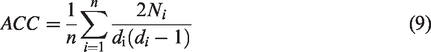
The average clustering coefficient is extensively implemented to assess the robustness of the network (Barthélemy, 2011; Ponton et al., 2013; Yao et al., 2018). In other words, it measures the network’s ability to withstand the deletion of its nodes. The average clustering coefficient is calculated using equation (9), where $|N_{i}|$ represents the number of links between node $i$ adjacent nodes and $d_{i}$ is the degree of node $i$ (Barthélemy, 2011)

ACC = \frac{1}{n} \sum_{i = 1}^{n} \frac{2 |N_{i}|}{d_{i} (d_{i} - 1)}

(9)

Network connectivity

Network connectivity has been extensively investigated in previous studies, where several measurements have been introduced (e.g. intersection density, network density, and network coverage). Two measures of connectivity are used in this study to quantify network connectivity: network density and intersection density. Network density is calculated as the proportion of the aggregated length of the bike links in a TAZ to the corresponding TAZ area. This measure was employed in previous studies for measuring network connectivity (Berrigan et al., 2010; Osama and Sayed, 2016; Saha et al., 2018; Schoner and Levinson, 2014; Zhang et al., 2012). Intersection density is the number of nodes (intersections) in a TAZ divided by the area of the corresponding TAZ. Previous research has introduced intersection density as a network connectivity metric (Cervero and Kockelman, 1997; Osama and Sayed, 2016; Zhang et al., 2012).

Network directness

Two measures are used to assess network directness: linearity and the average edge length. To measure linearity, theoretical links are created that characterize the length of the bike network in the case where all the links are straight while maintaining the nodes’ location. The aggregated length of the theoretical straight links is called modified bike network length. Linearity is then defined as the modified bike network length divided by the actual length of the bike network, for each TAZ. The average edge length is the total length of the bike network divided by the number of links in each TAZ (Kansky, 1963).

Topography

The total length of the bike network is estimated by summing up all the bike network link lengths while ignoring their types, i.e. separated, on-street, etc., within each TAZ. The average weighted slope of the bike network is the aggregated length weighted slope divided by the length of the bike network in each TAZ (Osama and Sayed, 2016).

Method

Model development

The FB approach has two main advantages in comparison to the traditional frequentist approach. First, it has the benefit of accounting for uncertainty and a more flexible framework that can be adjusted in compliance with the modeling process (El-Basyouny and Sayed, 2009). Second, because of its capability of dealing with complex correlations, the FB method is more appropriate for spatial modeling (Aguero-Valverde and Jovanis, 2008).

The FB model for BKT was created with a random error lognormally distributed. In this way, the error term, $u_{i}^{'}$ , can be represented as shown in equation (10). The final form of the model is shown in equation (11). The BKT model was estimated using lognormal regression, as the model should not yield a negative result, and the BKT distribution is right-skewed

u_{i}^{'} \sim Normal (0, σ_{u^{'}}^{2})

(10)

{\ln (BKT}_{i}) = b_{0} + Σ_{m} b_{m} X_{m i} + u_{i}^{'} + s_{i}^{'}

(11)

where

{BKT}_{i}

is the value of the

{i th}^{}

zone (

i = 1, \dots, ρ

ρ

is the number of zones,

u_{i}^{'}

is the unstructured heterogeneity between the zones,

s_{i}^{'}

accounts for the spatially correlated heterogeneity among the zones,

σ_{u^{'}}^{2}

is the unstructured heterogeneity variation

{, b}_{0}

is the intercept,

X_{m i}

represents the value of the

{m th}^{}

explanatory variable for the

{i th}^{}

zone,

m

is the number of the explanatory variables,

i

is the number of zones, and

b_{m}

is the model parameter for the

{m th}^{}

explanatory variable. For the model development process, some of the variables were highly correlated. Therefore, highly correlated variables were not included together in the same model. For example, the network connectivity indicators (e.g. intersection density and network density), are not used in the same model. After developing every possible model, only models with specifications where all the independent variables are credible at 10% were included as candidates, while the other tested models were discarded. From the candidate models, models with the lowest deviance information criterion (DIC) were reported.

The Poisson lognormal model is employed for the bike–vehicle crash models. Then spatial effects are employed to account for structured heterogeneities. The FB model procedure emulates the practice presented in El-Basyouny and Sayed (2009). $Y_{i}$ is the number of bike–vehicle crashes at zone $i$ , and it follows a Poisson distribution with a parameter $λ_{i}$ as shown in equation (12). $λ_{i}$ is treated as a random variable and modeled as shown in equation (13)

Y_{i} \sim Poisson (λ_{i})

(12)

\ln (λ_{i}) = a_{o} + a_{1} \ln ({VKT}_{i}) + a_{2} \ln ({BKT}_{i}) + {Σ_{m} d}_{m} Z_{m i} + u_{i}^{''} + s_{i}^{''}

(13)

where

a_{o}

a_{1}, a_{2},

and

d_{m}

are the model parameters,

{VKT}_{i}

and

{BKT}_{i}

are the vehicle and bike exposure variables, respectively,

Z_{m i}

represents the value of the

{m th}^{}

explanatory variable for the

{i th}^{}

zone,

u_{i}^{''}

represents the unstructured heterogeneities among the zones, and

s_{i}^{''}

represents the structured heterogeneities among the zones.

u_{i}^{''}

follows a lognormal distribution, as inferred from equations (13) and (14)

u_{i}^{''} \sim Normal (0, σ_{u^{''}}^{2})

(14)

where

σ_{u^{''}}^{2}

is the unstructured heterogeneity variance. The spatial effect for BKT and bike crash models is modeled by Gaussian Conditional Autoregressive Regressive techniques and calculated using equation (15), for each model separately

S_{i} | S_{- i} \sim Normal (\bar{s_{i}}, \frac{σ_{s}^{2}}{n_{i}}), where \bar{s_{i}} = \sum_{j ϵ C (i)} \frac{s_{j}}{{N i}_{i}}

(15)

where

σ_{s}^{2}

is the spatial variation,

{N i}_{i}

is the number of neighbors of zone

i

C (i)

is the set of neighbors of zone

i

S_{i}

accounts for the spatially correlated (structured) heterogeneity among zones, and

S_{- i}

is the set of all spatial effects except

S_{i}

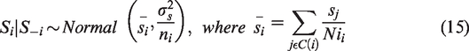
The spatial variation is assessed according to equation (16) (Aguero-Valverde and Jovanis, 2008)

ψ_{s} = \frac{σ_{s}^{2}}{σ_{s}^{2} + σ_{u}^{2}}

(16)

The FB model estimation follows El-Basyouny and Sayed (2009); for more details, please refer to the FB model estimation section of the online Supplementary Material. The model development process followed is like that of the BKT model development process.

Bayesian mediation analysis is employed to assess the mediated effects that bike network indicators may have on crashes through their effects on BKT by recognizing BKT as a mediator. Kamel et al. (2019) defined mediation analysis as follows:

Mediation analysis is used to estimate how a variable transmits its effects to another variable through a certain mediator. These effects could be direct only, indirect only (through a certain mediator), or both direct and indirect. Fully mediated variables are variables with indirect effect only.

The causal steps method is typically used in previous studies to conduct mediation analysis ( Baron and Kenny, 1986; Judd and Kenny, 1981), which is used in this study. Equation (17) represents the effects of x (bike network indicators) on m (BKT). Equation (18) represents the effect of m and x on y (cyclist–vehicle crashes). The indirect effect (τ) of x on y is assessed by equation (19) (Hayes, 2017; Yuan and MacKinnon, 2009). The total effect is computed by combining the indirect and direct effects as follows

m_{i} = δ_{0} + δ_{1} x_{i} + u_{i}^{'} + s_{i}^{'}

(17)

y_{i} = γ_{0} + γ_{1} m_{i} + γ_{2} x_{i} + u_{i}^{''} + s_{i}^{''}

(18)

τ = δ_{1} * γ_{1}

(19)

Results and discussion

Bike Kilometers Traveled models

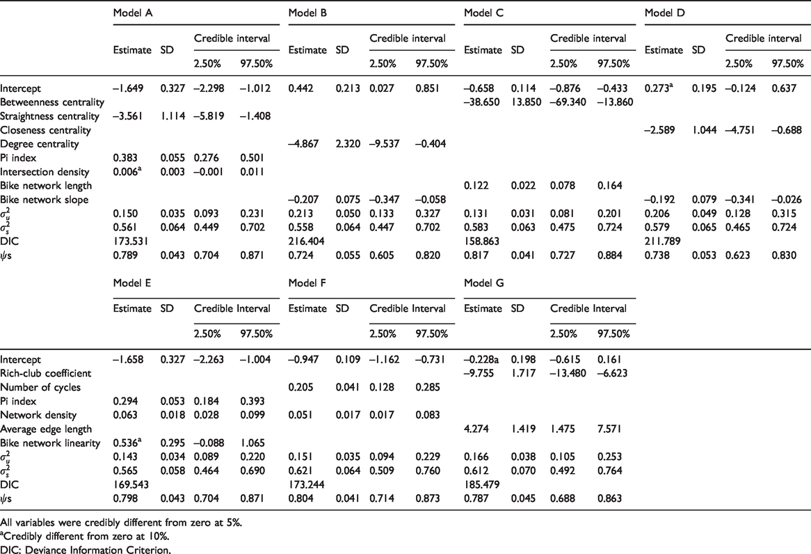
Table 1 presents the developed BKT FB models A–G. All the variables are statistically credible at the 5% or 10% level. Degree, betweenness, closeness, and straightness graph centralities have negative associations with the BKT. This is logical as high network centrality indicates low inter-connectivity and accessibility (Zhang et al., 2015). Furthermore, Marshall and Garrick (2010) found that gridded street networks (low centrality networks) were associated with higher walking and biking.

Table 1.

Full Bayes Bike Kilometers Traveled models (A–G).

	Model A				Model B				Model C				Model D
	Estimate	SD	Credible interval		Estimate	SD	Credible interval		Estimate	SD	Credible interval		Estimate	SD	Credible interval
			2.50%	97.50%			2.50%	97.50%			2.50%	97.50%			2.50%	97.50%
Intercept	–1.649	0.327	–2.298	–1.012	0.442	0.213	0.027	0.851	–0.658	0.114	–0.876	–0.433	0.273^a	0.195	–0.124	0.637
Betweenness centrality									–38.650	13.850	–69.340	–13.860
Straightness centrality	–3.561	1.114	–5.819	–1.408
Closeness centrality													–2.589	1.044	–4.751	–0.688
Degree centrality					–4.867	2.320	–9.537	–0.404
Pi index	0.383	0.055	0.276	0.501
Intersection density	0.006^a	0.003	–0.001	0.011
Bike network length									0.122	0.022	0.078	0.164
Bike network slope					–0.207	0.075	–0.347	–0.058					–0.192	0.079	–0.341	–0.026
$σ_{u}^{2}$	0.150	0.035	0.093	0.231	0.213	0.050	0.133	0.327	0.131	0.031	0.081	0.201	0.206	0.049	0.128	0.315
$σ_{s}^{2}$	0.561	0.064	0.449	0.702	0.558	0.064	0.447	0.702	0.583	0.063	0.475	0.724	0.579	0.065	0.465	0.724
DIC	173.531				216.404				158.863				211.789
ψs	0.789	0.043	0.704	0.871	0.724	0.055	0.605	0.820	0.817	0.041	0.727	0.884	0.738	0.053	0.623	0.830

	Model E				Model F				Model G
	Estimate	SD	Credible Interval		Estimate	SD	Credible Interval		Estimate	SD	Credible Interval
			2.50%	97.50%			2.50%	97.50%			2.50%	97.50%
Intercept	–1.658	0.327	–2.263	–1.004	–0.947	0.109	–1.162	–0.731	–0.228a	0.198	–0.615	0.161
Rich-club coefficient									–9.755	1.717	–13.480	–6.623
Number of cycles					0.205	0.041	0.128	0.285
Pi index	0.294	0.053	0.184	0.393
Network density	0.063	0.018	0.028	0.099	0.051	0.017	0.017	0.083
Average edge length									4.274	1.419	1.475	7.571
Bike network linearity	0.536^a	0.295	–0.088	1.065
$σ_{u}^{2}$	0.143	0.034	0.089	0.220	0.151	0.035	0.094	0.229	0.166	0.038	0.105	0.253
$σ_{s}^{2}$	0.565	0.058	0.464	0.690	0.621	0.064	0.509	0.760	0.612	0.070	0.492	0.764
DIC	169.543				173.244				185.479
ψs	0.798	0.043	0.704	0.871	0.804	0.041	0.714	0.873	0.787	0.045	0.688	0.863

All variables were credibly different from zero at 5%.

^aCredibly different from zero at 10%.

DIC: Deviance Information Criterion.

The rich-club coefficient is negatively associated with BKT. In other words, networks where highly connected nodes are connected (“The rich get richer”) have low bike traffic. When systemically connected nodes are getting more connections, the network forces cyclists through traffic dense intersections (highly connected nodes). This situation may deter bikes, as it lengthens their trips. Also, cyclists may perceive it as a less safe network as it forces bikes toward intersections with many conflict points with road users.

The Pi index and the number of network cycles are positively associated with BKT. This is logical as developed networks encourage road users to cycle, which is consistent with previous findings (Buehler and Pucher, 2012; Dill and Carr, 2003; Nelson and Allen, 1997; Winters et al., 2016).

Intersection density and network density are positively associated with BKT, which is in line with previous studies (Berrigan et al., 2010; Marshall and Garrick, 2010; Osama et al., 2017; Schoner and Levinson, 2014) in which they showed that connectivity and density are positively associated with biking levels. Linearity and average edge length are positively associated with BKT. This is consistent with Schoner and Levinson (2014) and Osama et al. (2017), where they showed that a continuous network with fewer hindrances is positively associated with biking levels. The bike network length is positively associated with BKT, which is intuitive, as more bike infrastructure usually yields more bike trips (Buehler and Pucher, 2012; Dill and Carr, 2003; Nelson and Allen, 1997 ; Osama et al., 2017; Winters et al., 2016). The average weighted slope is negatively associated with BKT; this is also intuitive and consistent with previous studies (Hood et al., 2011; Osama et al., 2017; Winters et al., 2016), as steeper slopes work as a deterrent for bikes.

The assortativity coefficient and the average clustering coefficient have non-credible negative and positive associations with the BKT, respectively. The DIC of Model C is credibly lower than the other models as the difference between Model C and the second-best model (Model E) is 10.680. This indicates that Model C has the best performance compared to the other models developed here. Future studies should investigate the best-fitted model after including other relevant variables such as land use, demographics, and the street network. The variation associated with the spatial term $σ_{s}^{2}$ is credibly higher than the variation associated with the unstructured heterogeneity term $σ_{u}^{2}$ . Also, the spatial variation ψs shows that the proportion of spatial variation is higher than the proportion of the unobserved heterogeneity to the total variation. This shows the importance of including the spatial term in the models.

Correlated variables were restricted from being included in the same model to avoid multicollinearity, which may lead to biased and insignificant estimates. Multicollinearity makes it difficult to determine which variables (out of the correlated variables) are causal and which are the result of illusory correlation (Washington et al., 2010).

Bike–vehicle crash models

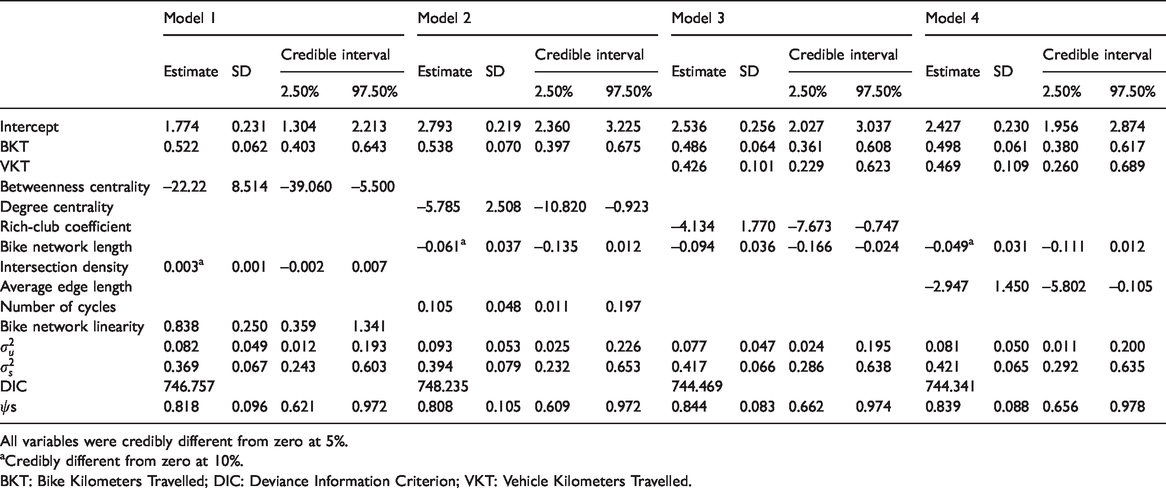
Table 2 presents the FB crash models 1–4. All the variables are statistically credible at the 5% or 10% levels. Vehicle kilometers traveled and BKT are found to be positively associated with bike–vehicle crashes. This is expected and consistent with previous research (Hamann and Peek-Asa, 2013; Kaplan and Prato, 2015; Miranda-Moreno et al., 2011; Strauss et al., 2013).

Table 2.

Full Bayes bike–vehicle crash models 1–4.

	Model 1				Model 2				Model 3				Model 4
	Estimate	SD	Credible interval		Estimate	SD	Credible interval		Estimate	SD	Credible interval		Estimate	SD	Credible interval
			2.50%	97.50%			2.50%	97.50%			2.50%	97.50%			2.50%	97.50%
Intercept	1.774	0.231	1.304	2.213	2.793	0.219	2.360	3.225	2.536	0.256	2.027	3.037	2.427	0.230	1.956	2.874
BKT	0.522	0.062	0.403	0.643	0.538	0.070	0.397	0.675	0.486	0.064	0.361	0.608	0.498	0.061	0.380	0.617
VKT									0.426	0.101	0.229	0.623	0.469	0.109	0.260	0.689
Betweenness centrality	–22.22	8.514	–39.060	–5.500
Degree centrality					–5.785	2.508	–10.820	–0.923
Rich-club coefficient									–4.134	1.770	–7.673	–0.747
Bike network length					–0.061^a	0.037	–0.135	0.012	–0.094	0.036	–0.166	–0.024	–0.049^a	0.031	–0.111	0.012
Intersection density	0.003^a	0.001	–0.002	0.007
Average edge length													–2.947	1.450	–5.802	–0.105
Number of cycles					0.105	0.048	0.011	0.197
Bike network linearity	0.838	0.250	0.359	1.341
$σ_{u}^{2}$	0.082	0.049	0.012	0.193	0.093	0.053	0.025	0.226	0.077	0.047	0.024	0.195	0.081	0.050	0.011	0.200
$σ_{s}^{2}$	0.369	0.067	0.243	0.603	0.394	0.079	0.232	0.653	0.417	0.066	0.286	0.638	0.421	0.065	0.292	0.635
DIC	746.757				748.235				744.469				744.341
ψs	0.818	0.096	0.621	0.972	0.808	0.105	0.609	0.972	0.844	0.083	0.662	0.974	0.839	0.088	0.656	0.978

All variables were credibly different from zero at 5%.

^aCredibly different from zero at 10%.

BKT: Bike Kilometers Travelled; DIC: Deviance Information Criterion; VKT: Vehicle Kilometers Travelled.

The betweenness and degree centralities have a negative association with bike–vehicle crashes. This is consistent with previous research (Zhang et al., 2015) and largely intuitive. A network with low centrality indicates high inter-connectivity and accessibility. High connectivity promotes vehicle accessibility that encourages intra-zonal trips, which take place through collectors and local roads instead of arterial roads. Since collectors and local roads are usually designed for low volume and low-speed traffic, therefore, combining this traffic with local bike traffic has been shown to impact road safety negatively (Lovegrove and Sayed, 2006).

The rich-club coefficient has negative associations with bike–vehicle crashes. One possible explanation is that cyclists are forced onto major links and nodes where usually risk mitigation measures are applied. However, such results need to be further investigated with out-of-sample or longitudinal data.

The number of cycles has a positive association with bike–vehicle crashes. These results indicate that network complexity decreases bike safety. This may be attributed to complex and developed networks creating more conflict points between vehicles and bikes.

The intersection density has positive associations with bike–vehicle crashes. This is expected and consistent with previous research (Siddiqui et al., 2012; Strauss et al., 2013; Wei and Lovegrove, 2013; Osama and Sayed, 2016; Chen et al., 2018). The positive association of intersection density with bike–vehicle crashes may be attributed to the fact that bike–vehicle interactions are high at the intersections, which would lead to increased crash risk. The average edge length has a negative association with bike–vehicle crashes. The results imply that elongated paths have links with fewer intersections and are safer for bikes. This agrees with the previous study conducted by Quintero et al. (2013) in which they explore the Metro Vancouver transit network. Moreover, the increase in linearity is correlated with an increase in bike–vehicle crashes, which may be accredited to the propensity of vehicles and bikes to increase their speed on straight links, which would increase bike–vehicle crash risk. The bike network length has a negative association with bike–vehicle crashes. This is consistent with previous studies’ findings, where it is concluded that more bike infrastructure would increase bike safety (Kaplan et al., 2014; Prato et al., 2016; Rome et al., 2014).

The straightness and closeness centralities as well as the assortativity coefficient have non-credible negative associations with bike–vehicle crashes. The Pi index, average clustering coefficient, network density, and weighted slope have non-credible positive associations with bike–vehicle crashes. Comparing the DIC values for the developed models indicates that there is no significant difference in model performance between the developed models. Like the BKT model, $σ_{s}^{2}$ , $σ_{u}^{2}$ , and ψ_s show the importance of including the spatial term in the models developed here.

Several bike network indicators (centrality, complexity, connectivity, directness, and topography) are credibly associated with BKT, and BKT is credibly associated with bike–vehicle crashes. BKT works as a mediator (mediating an impact of bike network indicators on bike–vehicle crashes) while the bike network indicators have mediated effects (indirect effects) on bike–vehicle crashes. To compare bike network indicators’ direct effects on bike–vehicle crashes and total effects (the aggregation of the direct and indirect effects), the indirect effect of bike network indicators on bike–vehicle crashes was evaluated. Mediation analysis shows that some bike network indicators have different direct and indirect effects on bike–vehicle crashes while other indicators have a consistent effect on bike–vehicle crashes, as shown in Table S3 in the online Supplementary Material. However, bike network indicators’ direct and total effects have the same impact direction (estimates’ sign) on bike–vehicle crashes.

Conclusion and summary

The study developed zone-level BKT models and bike–vehicle crash models using FB techniques incorporating spatial effects. A set of network theory indicators were introduced to quantify bike network features. The bike network indicators were divided into seven categories: centrality, assortativity, complexity, robustness, connectivity, directness, and topography.

The developed BKT models showed that bike network centrality, assortativity, and weighted slope have a negative association with BKT, while bike network directness, length, complexity and development, and connectivity have a positive association with BKT. The developed crash models show that the bike network length, centrality, assortativity, and continuity have negative associations with bike–vehicle crashes. On the other hand, bike network complexity and development, connectivity, and linearity have positive associations with bike–vehicle crashes.

The results indicate that increases in bike network length and network continuity are expected to increase BKT and decrease bike–vehicle crashes. On the other hand, while enhancing zone attractiveness to bikes by adjusting bike network centrality, assortativity, complexity, connectivity, and linearity, network planners should be careful as these indicators have a contradictory effect on bike safety. Therefore, adjusting these network indicators should be accompanied by risk mitigation measures.

This study comes with some limitations. The network theory indicators investigated in this study describe the bike network’s infrastructure, but they do not account for the built environment context surrounding the bicycle network, such as land use, socioeconomic factors, and road facilities. Osama et al. (2017) have studied the impact of land use, socioeconomic factors, and road facility variables on bike–vehicle crashes using the same data set. In other words, this study is limited to quantification of bike lanes (on-street and off-street bike lanes), without consideration of the surrounding facilities (e.g. bike racks, shoulder location and other characteristics, on-street car parking, etc.). This study treated off-street and on-street bike lanes interchangeably as they provide a designated space for bikes. However, cyclists may value (or treat) these facility types differently. This study considered only bike–vehicle crashes due to data limitations. Investigating other types of crashes such as bike–bike or bike–pedestrian crashes would be beneficial. The data used in the study are from a medium–low bike-use community. Therefore, studies are needed from cities and regions with complete bikeway networks and higher bike-use communities, most probably in European countries, to further investigate the impact of bike network infrastructure on biking activity level and safety. Future research should investigate the association of the presented network indicators with motorists’ safety and ridership, as well as pedestrians’ safety and walkability.

Supplemental Material

sj-pdf-1-epb-10.1177_2399808320964469 - Supplemental material for The impact of bike network indicators on bike kilometers traveled and bike safety: A network theory approach

Supplemental material, sj-pdf-1-epb-10.1177_2399808320964469 for The impact of bike network indicators on bike kilometers traveled and bike safety: A network theory approach by Mohamed Bayoumi Kamel and Tarek Sayed in Environment and Planning B: Urban Analytics and City Science

Footnotes

Declaration of conflicting interests

The author(s) declared no potential conflicts of interest with respect to the research, authorship, and/or publication of this article.

Funding

The author(s) received no financial support for the research, authorship, and/or publication of this article.

ORCID iD

Mohamed Bayoumi Kamel

Supplemental material

Supplemental material for this article is available online.

Mohamed Bayoumi Kamel is currently a PhD candidate in the Civil Engineering Department at the University of British Columbia. His current research is focused on investigating the built environment effect on bike ridership as well as biking safety.

Tarek Sayed is currently a Professor and a Distinguished Scholar with the Department of Civil Engineering, The University of British Columbia. His transportation engineering research has been focused on three main areas: to improve road safety analysis and evaluation techniques; to improve the level of knowledge associated with the safety implications of traffic operations and highway design, as well as, developing and evaluating intelligent transportation systems to increase the efficiency of traffic. He is a fellow of the Engineering Institute of Canada, the Canadian Academy of Engineering, and the Canadian Society for Civil Engineering.

References

Aguero-Valverde

Jovanis

(2008) Analysis of road crash frequency with spatial models. Transportation Research Record: Journal of the Transportation Research Board 2061: 55–63.

Baron RM and

Kenny

(1986) The Moderator-Mediator Variable Distinction in Socialpsychological Research: Conceptual Strategic, and Statistical Considerations. J Pers Soc Psychol 51: 1173.

Barthélemy

(2011) Spatial networks. Physics Reports 499: 1–101.

Berrigan

Pickle

Dill

(2010) Associations between street connectivity and active transportation. International Journal of Health Geographics 9: 20.

Buehler

Pucher

(2012) Cycling to work in 90 large American cities: New evidence on the role of bike paths and lanes. Transportation 39: 409–432.

Cervero

Kockelman

(1997) Travel demand and the 3Ds: Density, diversity, and design. Transportation Research Part D: Transport and Environment 2: 199–219.

Chen

Srinivasan

, et al. (2012) Evaluating the safety effects of bicycle lanes in New York city. American Journal of Public Health 102: 1120–1127.

Chen

(2015) Built environment factors in explaining the automobile-involved bicycle crash frequencies: A spatial statistic approach. Safety Science 79: 336–343.

Chen

Sun

Wang

, et al. (2018) Built environment effects on bike crash frequency and risk in Beijing. Journal of Safety Research 64: 135–143.

10.

Cho

Rodríguez

Khattak

(2009) The role of the built environment in explaining relationships between perceived and actual pedestrian and bicyclist safety. Accident Analysis and Prevention 41: 692–702.

11.

Crucitti

Latora

Porta

(2006) Centrality measures in spatial networks of urban streets. Physical Review. E, Statistical, Nonlinear, and Soft Matter Physics 73: 036125.

12.

De Montis

Barthélemy

Chessa

, et al. (2007) The structure of interurban traffic: A weighted network analysis. Environment and Planning B: Planning and Design 34: 905–924.

13.

Dill

Carr

(2003) Bicycle commuting and facilities in major US cities: If you build them, commuters will use them. Transportation Research Record: Journal of the Transportation Research Board 1828: 116–123.

14.

El-Basyouny

Sayed

(2009) Urban arterial accident prediction models with spatial effects. Transportation Research Record: Journal of the Transportation Research Board 2102: 27–33.

15.

El Esawey

Lim

Sayed

(2015) Development of a cycling data model: City of Vancouver case study. Canadian Journal of Civil Engineering 42: 1000–1010.

16.

Freeman

(1978) Centrality in social networks conceptual clarification. Social Networks 1: 215–239.

17.

Hamann

Peek-Asa

(2013) On-road bicycle facilities and bicycle crashes in Iowa, 2007–2010. Accident Analysis and Prevention 56: 103–109.

18.

Handy

Xing

(2011) Factors correlated with bicycle commuting: A study in six small U.S. cities. International Journal of Sustainable Transportation 5: 91–110.

19.

Harris

Reynolds

CCO

Winters

, et al. (2011) The bicyclists’ injuries and the cycling environment study: A protocol to tackle methodological issues facing studies of bicycling safety. Injury Prevention 17(5): e6.

20.

Hayes

(2017) Introduction to Mediation, Moderation, and Conditional Process Analysis: A Regression-Based Approach. New York: Guilford Publications.

21.

Hood

Sall

Charlton

(2011) A GPS-based bicycle route choice model for San Francisco, California. Transportation Letters 3: 63–75.

22.

Jayasinghe

Sano

Nishiuchi

(2015) Explaining traffic flow patterns using centrality measures. International Journal for Traffic and Transport Engineering 5(2): 134–149.

23.

Jiang

(2009) Street hierarchies: A minority of streets account for a majority of traffic flow. International Journal of Geographical Information Science 23: 1033–1048.

24.

Jiang

Duan

, et al. (2014) Topological structure of urban street networks from the perspective of degree correlations. Environment and Planning B: Planning and Design 41: 813–828.

25.

Judd C M and

Kenny

D A

(1981) Process Analysis: Estimating Mediation in Treatment Evaluations. Evaluation Review 5(5): 602.

26.

Kamel

Sayed

(2020) Cyclist-vehicle crash modeling with measurement error in traffic exposure. Accident Analysis and Prevention 144: 105612.

27.

Kamel

Sayed

Bigazzi

(2020) A composite zonal index for biking attractiveness and safety. Accident Analysis and Prevention 137: 105439.

28.

Kamel

Sayed

Osama

(2019) Accounting for mediation in cyclist-vehicle crash models: A Bayesian mediation analysis approach. Accident Analysis and Prevention 131: 122–130.

29.

Kansky

(1963) Structure of Transportation Networks: Relationships between Network Geometry and Regional Characteristics. Chicago: University of Chicago.

30.

Kaplan

Prato

(2015) A spatial analysis of land use and network effects on frequency and severity of cyclist–motorist crashes in the Copenhagen region. Traffic Injury Prevention 16: 724–731.

31.

Kaplan

Vavatsoulas

Prato

(2014) Aggravating and mitigating factors associated with cyclist injury severity in Denmark. Journal of Safety Research 50: 75–82.

32.

Lovegrove

Sayed

(2006) Macro-level collision prediction models for evaluating neighbourhood traffic safety. Canadian Journal of Civil Engineering 33: 609–621.

33.

Marshall

Garrick

(2010) Effect of street network design on walking and biking. Transportation Research Record: Journal of the Transportation Research Board 2198: 103–115.

34.

Mekuria

Furth

Nixon

(2012) Low-stress bicycling and network connectivity. MTI Report 11-19. San Jose: Mineta Transportation Institute.

35.

Miranda-Moreno

Strauss

Morency

(2011) Disaggregate exposure measures and injury frequency models of cyclist safety at signalized intersections. Transportation Research Record: Journal of the Transportation Research Board 2236: 74–82.

36.

Nelson

Allen

(1997) If you build them, commuters will use them: Association between bicycle facilities and bicycle commuting. Transportation Research Record: Journal of the Transportation Research Board 1578(1): 79–83.

37.

Newman

MEJ

(2002) Assortative mixing in networks. Physical Review Letters 89: 208701.

38.

Newman

MEJ

(2003) Mixing patterns in networks. Physical Review E: Statistical, Nonlinear, and Soft Matter Physics 67: 026126.

39.

Osama

Sayed

(2016) Evaluating the impact of bike network indicators on cyclist safety using macro-level collision prediction models. Accident Analysis and Prevention 97: 28–37.

40.

Osama

Sayed

Bigazzi

(2017) Models for estimating zone-level bike kilometers traveled using bike network, land use, and road facility variables. Transportation Research Part A: Policy and Practice 96: 14–28.

41.

Ponton

Wei

Sun

(2013) Weighted clustering coefficient maximization for air transportation networks. In: 2013 European Control Conference (ECC), 17–19 July 2013, pp.866–871. Zurich, Switzerland. IEEE.

42.

Porta

Crucitti

Latora

(2006) The network analysis of urban streets: A primal approach. Environment and Planning B: Planning and Design 33: 705–725.

43.

Porta

Latora

Wang

, et al. (2012) Street centrality and the location of economic activities in Barcelona. Urban Studies 49: 1471–1488.

44.

Prato

Kaplan

Rasmussen

, et al. (2016) Infrastructure and spatial effects on the frequency of cyclist-motorist collisions in the Copenhagen region. Journal of Transportation Safety & Security 8: 346–360.

45.

Quintero

Sayed

Wahba

(2013) Safety models incorporating graph theory based transit indicators. Accident Analysis and Prevention 50: 635–644.

46.

Rodrigue

J-P

Comtois

Slack

(2013) The Geography of Transport Systems. 3rd ed. London, New York: Routledge.

47.

Rome

Boufous

Georgeson

, et al. (2014) Bicycle crashes in different riding environments in the Australian Capital Territory. Traffic Injury Prevention 15: 81–88.

48.

Saha

Alluri

Gan

, et al. (2018) Spatial analysis of macro-level bicycle crashes using the class of conditional autoregressive models. Accident Analysis and Prevention 118: 166–177.

49.

Schoner

Levinson

(2014) The missing link: Bicycle infrastructure networks and ridership in 74 US cities. Transportation 41: 1187–1204.

50.

Siddiqui

Abdel-Aty

Choi

(2012) Macroscopic spatial analysis of pedestrian and bicycle crashes. Accident Analysis and Prevention 45: 382–391.

51.

Strauss

Miranda-Moreno

Morency

(2013) Cyclist activity and injury risk analysis at signalized intersections: A Bayesian modelling approach. Accident Analysis and Prevention 59: 9–17.

52.

Washington

Karlaftis

Mannering

(2010) Statistical and Econometric Methods for Transportation Data Analysis. London: Chapman and Hall/CRC.

53.

Wei

Lovegrove

(2013) An empirical tool to evaluate the safety of cyclists: Community based, macro-level collision prediction models using negative binomial regression. Accident Analysis and Prevention 61: 129–137.

54.

Winters

Teschke

Brauer

, et al. (2016) Bike score®: Associations between urban bikeability and cycling behavior in 24 cities. The International Journal of Behavioral Nutrition and Physical Activity 13: 18.

55.

Yao

Hong

, et al. (2018) Estimating the effects of “community opening” policy on alleviating traffic congestion in large Chinese cities by integrating ant colony optimization and complex network analyses. Computers, Environment and Urban Systems 70: 163–174.

56.

Yasmin

Eluru

(2016) Latent segmentation based count models: Analysis of bicycle safety in Montreal and Toronto. Accident Analysis and Prevention 95: 157–171.

57.

Yuan

MacKinnon

(2009) Bayesian mediation analysis. Psychological Methods 14: 301–322.

58.

Zhang

Bigham

, et al. (2012) Associations between road network connectivity and pedestrian-bicyclist accidents. In: 91st Annual Meeting of the Transportation Research Board, 22–26 January 2012, Washington DC.

59.

Zhang

Bigham

Ragland

, et al. (2015) Investigating the associations between road network structure and non-motorist accidents. Journal of Transport Geography 42: 34–47.

60.

Zhang

Wang

Zeng

, et al. (2011) Centrality characteristics of road network patterns of traffic analysis zones. Transportation Research Record: Journal of the Transportation Research Board 2256: 16–24.

61.

Zhou

Mondragon

(2004) The rich-club phenomenon in the Internet topology. IEEE Communications Letters 8: 180–182.

Supplementary Material

Please find the following supplemental material available below.

For Open Access articles published under a Creative Commons License, all supplemental material carries the same license as the article it is associated with.

For non-Open Access articles published, all supplemental material carries a non-exclusive license, and permission requests for re-use of supplemental material or any part of supplemental material shall be sent directly to the copyright owner as specified in the copyright notice associated with the article.

0.00 MB

0.52 MB