Spatial sensitivity analysis for urban hotspots using cell phone traces

Abstract

Urban hotspots can be used to model the structure of urban environments and to study or predict various aspects of urban life. An increasing interest in the analysis of urban hotspots has been triggered by the emergence of pervasive technologies that produce massive amounts of spatio-temporal data including cell phone traces (or Call Detail Records). Although hotspot analyses using cell phone traces are extensive, there is no consensus among researchers about the process followed to compute them in terms of four important methodological choices: city boundaries, spatial units, interpolation methods, and hotspot variables. Using a large-scale CDR dataset from Mexico, we provide an interpretable systematic spatial sensitivity analysis of the impact that these methodological choices might have on the stability of the hotspot variables in both static and dynamic settings.

Keywords

Spatial sensitivity analysis urban hotspots cell phone traces

Introduction

Urban environments can be characterized using different approaches, such as land use, mobility matrices, or activity centers (a.k.a. hotposts). The recent availability of pervasive technologies has triggered new ways of studying cities using different data sources such as social networks, GPS, public transport information, and also cell phone traces.

Cell phone traces (or Call Detail Records, CDRs) are collected by telecommunication networks for billing purposes and provide—among other features—spatio-temporal data about mobility behavior. CDR data have been proved to be useful in modeling a variety of human mobility behaviors such as analyzing daily patterns to understand the pulse of a city (Ahas et al., 2015; Ratti et al., 2006; Reades et al., 2007); investigating the correlation between human mobility patterns and land-use patterns as well as urban functions (Bachir et al., 2017; Reades et al., 2007); or clustering geographic units as dense regions to understand city dynamics at large scale (Doyle et al., 2014; Vieira et al., 2010).

A critical area in mobility behavior analysis is the identification of regions of interest (ROI) or dense regions a.k.a. hotspots, defined as regions with high concentration of individuals for a given period of time (Chen et al., 2019; Hoteit et al., 2014; L3Harris, n.d.; Louail et al., 2014; Ratti et al., 2006; Vieira et al., 2010). Hotspot analyses using CDR data are generally carried out in two different scenarios: (1) modeling, with a focus on analyzing the urban structure, such as the quantification of the urban sprawl or compactness of cities (Louail et al., 2014; Xu et al., 2019), or the analysis of the spatio-temporal evolution of popular locations for a given region (Ghahramani et al., 2018; Zuo and Zhang, 2012); and (2) prediction, with a focus on the analysis of the predictive power of dense regions with respect to a given variable; for example, high footfall (number of estimated visits) in a region has been associated to high crime (Bogomolov et al., 2015; Traunmueller et al., 2014), or large numbers of individuals at night or work times have been associated to the identification of home (residential) and work locations (Isaacman et al., 2012). These studies are often carried out at two different spatial scales: intra-city, where researchers focus on spatio-temporal models or predictions for a given city (Ratti et al., 2006; Reades et al., 2007) and inter-city, where researchers focus on comparing static behaviors (one-time snapshots) across cities (Ahas et al., 2015; Louail et al., 2014).

Although hotspot analyses using cell phone traces are extensive, there is no consensus among researchers about the process followed to compute them in terms of three important features: (i) city boundaries used to define the area under study, e.g., some researchers use metropolitan areas (Louail et al., 2014) that represent cities as labor market areas comprising commuting behaviors, while others use a smaller entity—the core municipality—which represents the physical boundary of a city rather than its economic activity, and which is generally contained within a metropolitan area together with other non-core municipalities (Demographia, 2020; Ratti et al., 2006); (ii) spatial units considered to compute the hotspots, which in the literature range from using Voronoi polygons that simulate cell phone coverage areas (Doyle et al., 2014; Vieira et al., 2010); to uniformly distributed grids (Isaacman et al., 2012; Louail et al., 2014; Reades et al., 2007); or census tracts (Bachir et al., 2017; Doyle et al., 2014), with the latter two approaches requiring the use of interpolation methods (Ahas et al., 2015; Bachir et al., 2017; Kubíček et al., 2019; Peredo et al., 2017) to distribute individuals associated to a given cellular tower across grids or census tracts; and (iii) hotspot variables used to measure and characterize hotspots, such as the urban sprawl and compactness measures (Angel et al., 2010; Louail et al., 2014).

The combination of these different features could produce significant differences in the static and dynamic hotspots identified, i.e., urban hotspots could be sensitive to these methodological choices, which could in turn produce conflicting findings in the hotspot analyses or in its relationship with other urban characteristics. For example, a researcher interested in comparing the number of hotspots across cities could identify largely different city-rankings depending on the sets of features used. On the other hand, a researcher interested in using spatio-temporal hotspots to predict crime in a city could find a strong correlation or no correlation at all between hotspots and crime, depending on the set of city boundaries, spatial units, interpolation methods, and hotspot variables considered.

In this paper, we provide a spatial sensitivity analysis for urban hotspots computed using cell phone traces (CDR) in terms of three important spatial features: city boundaries, spatial units, and interpolation methods. The spatial sensitivity is quantified by a novel, interpretable hotspot index stability score that measures changes in hotspot variables via statistical ranking correlation. Highly stable combinations of spatial features will produce stable hotspot measures across settings, i.e., hotspot measures will not change across different combinations of features. The analysis presented in this paper will provide guidelines for researchers looking to identify the most stable (less sensitive) combination of parameters that will preserve the stability of the CDR-based hotspots independently of the city boundaries, spatial units, and interpolation methods selected; and will also pinpoint into risky combinations of features that might produce non-stable, CDR-based hotspot measures, i.e., measures that are highly sensitive to methodological choices.

The systematic analysis will be carried out for two settings: inter-city and intra-city, where most of the related literature in CDR-based hotspot analyses has focused. Inter-city analyses will evaluate the stability of the city-rankings, based on a given hotspot variable, across different combinations of city boundaries, spatial units and interpolation methods; while intra-city analyses will focus on a dynamic sensitivity analysis of the impact that different methodological choices have on the urban dynamics represented by the distribution of spatio-temporal hotspots in a city. As a result, the spatial sensitivity analysis presented in this paper will provide insights into the spatial sensitivity of traditional methodological choices in both static and dynamic settings.

Methodology

Hotspot analyses using CDR data are critical to study city dynamics and the spatial structure of cities. To detect hotspots, researchers generally follow a set of common steps, although its implementation varies widely depend on research focus, application area, or data availability. In this section, we will explain the different choices that researchers have in hand when computing hotspots, and we will describe the methodology we will use to assess the static and dynamic spatial sensitivity, i.e., the impact that the choice of varying feature combinations might have on the stability of a given hotspot measurement variable, both in static (inter-city) and dynamic (intra-city) settings.

Researchers generally follow these four steps to the identify the hotspots in a region: (i) define the city boundary of the city under study, (ii) define the type of spatial units used to compute hotspots, and estimate the population for each spatial unit, (iii) detect the static or dynamic hotspots based on the estimated population, and (iv) compute hotspot indices to quantitatively characterize, statically or dynamically, crowded regions in a city (see Figure 1 for details).

Figure 1.

Hotspot identification process. The gray areas in Step 1 are the areas considered in each city boundary setting, e.g., the gray areas in Urban settings are urban areas, while the white areas are the rural areas. The outer boundary is the metro area boundary and the inner boundaries are the municipalities’ boundaries.

City boundaries

The delimitation of cities or urban areas is in itself one of the traditional tasks in urban geography and planning (Ouředníček et al., 2018). Although not the focus of this paper, it highlights the importance of understanding the impact that different city delimitations might have on hotspot analyses. Most related studies focused on the computation of CDR-based hotspots consider two different dimensions.

The first one is the definition of the physical city boundary. While some researchers define cities by their metropolitan area (Gariazzo et al., 2019; Louail et al., 2014), others only consider the urban core (Chen et al., 2018; Kubíček et al., 2019; Ratti et al., 2006). Metropolitan areas are often defined as an aggregation of municipalities that share industry, infrastructure, and housing and that represent the economic city with a densely populated urban core area—that might span across multiple municipalities—and its surrounding rural, less-populated areas. On the other hand, municipalities are generally smaller spatial units embedded within a metropolitan area, with its urban core representing the physical boundary of the city and the region that has emerged historically as the most prominent in the metropolitan area (Demographia, 2020). Therefore, when the term city is used in current CDR-based hotspot analyses, it is important to understand whether it refers only to the densely populated areas within a metropolitan area (Chen et al., 2018; Ratti et al., 2006); or to the metropolitan area as a whole, including both the densely populated urban area and its less-populated, rural surrounding territories (Gariazzo et al., 2019; Le Néchet, 2012; Louail et al., 2014). See Urban and UrbanRural columns in Figure 1.

The second dimension focuses on whether to treat the metropolitan area as a whole unit to compute hotspots, or to consider each embedded municipality independent of each other, albeit connected by secondary population flows. Since metropolitan areas delimit the economic city, with mobility flows between its core urban area and other regions, it makes sense to identify hotspots at that scale, which would mostly characterize the commuting population (Le Néchet, 2012; Louail et al., 2014). However, by computing hotspots at that scale, local characteristics or economic structures of individual municipalities might be ignored. For example, non-core municipalities within a metropolitan area might be sub-centers for jobs in the region (Ouředníček et al., 2018). As a result, the mobility patterns characterizing these municipalities might be more affected by its internal flows that by movements to and from other municipalities (Gariazzo et al., 2019).

To carry out a comprehensive assessment of the different city boundary settings that are used by researchers when computing CDR-based hotspots, we propose to explore the following four settings: (i) Metropolitan Area Urban-Rural (Metro-UR), where hotspots are computed across the whole metropolitan area that includes all urban and rural areas; (ii) Metropolitan Area Urban (Metro-U), where hotspots are computed across the whole metropolitan area which is defined exclusively by its urban areas; (iii) Municipalities Urban-Rural (PerMuni-UR), where hotspots are computed per individual municipality, and considering both urban and rural areas within the municipality; and (iv) Municipalities Urban (PerMuni-U), where hotspots are computed individually only for the urban areas within each municipality. The boundary setting is denoted as b with $b \in$ {Metro-UR, Metro-U, PerMuni-UR, PerMuni-U}. An example of the four different boundary types is shown in Step 1 in Figure 1.

Spatial units and interpolation methods

Voronoi tessellation is a common spatial unit of choice when using CDR data to understand population dynamics (Doyle et al., 2014; Vieira et al., 2010). For each cell tower c in the cell phone infrastructure, Voronoi tesselation is used to represent its spatial coverage or service area (see Supp. Fig. 1). The assumption on which Voronoi tessellation is based is that users would always use the closest cell tower. In this way, researchers associate to a given Voronoi polygon v_c all the individuals that have been observed at that cell tower c. However, Voronoi polygons (Vor) are not the only type of relevant spatial units. Some researchers have focused on spatial regularity and have chosen grids (G) (Isaacman et al., 2012; Louail et al., 2014; Reades et al., 2007), while others prefer to census tracts or blocks (CT) (Bachir et al., 2017; Doyle et al., 2014) because these are the same geographic units as census data and can represent the boundaries of neighborhoods to some extent. In this paper, we will denote the type of spatial unit as t with $t \in {CT, G, Vor}$ .

Voronoi tessellation assigns a set of individuals to a given Voronoi polygon, and the number of individuals, i.e., the footfall, is then used to compute hotspots. However, when using grids or census tracts, or when a Voronoi polygon needs to be clipped because it spreads outside the boundary of a city or a municipality, additional processing is required to assign the presence of individuals to a different spatial unit. Grid and census tracts polygons will overlap with Voronoi polygons, and as a result, interpolation methods that approximate the footfall in a given overlapping polygon area is required (see Supp. Fig. 1 for an example). Similarly, clipped Voronoi polygons will require to approximate the footfall for any given sub-polygon. With that objective in mind, we explore three types of interpolation methods commonly present in the literature: uniform (Uni), population-based (Pop) and inverse-distance weighting (Idw) (Bachir et al., 2017; Louail et al., 2014; Peredo et al., 2017). In this paper, we will denote the interpolation methods as i with $i \in$ {Uni, Pop, Idw}.

The most common interpolation method in the CDR literature is the uniform method (Uni) (Kang et al., 2012; Kubíček et al., 2019; Louail et al., 2014). This method assumes that all individuals are located within a given polygon uniformly. Therefore, the number of individuals in any grid or census tract polygon overlapping with a Voronoi polygon will be proportional to its area.

The limitation of the Uniform method is that people are unlikely to be distributed over a spatial unit uniformly, especially for vast rural areas where people are less likely to be present. Therefore, researchers have used population-based methods (Pop) that distribute the footfall of a Voronoi polygon over a spatial unit proportionally to the population density, e.g., urban areas in the spatial unit are assigned larger numbers of individuals than rural areas (Bachir et al., 2017).

Nevertheless, the population-based method has an important drawback since the population retrieved from the census will represent residential population rather that footfall, which might affect the way population dynamics in non-residential areas are computed. Also, both uniform and population-based methods assume that the association of individuals to the closest cell tower location is always correct, which might not be the case specially for users who are at the boundaries of a given Voronoi polygon. Thus, researchers have used a third method to overcome these limitations, the inverse distance weighting (Idw) (Ahas et al., 2015; Peredo et al., 2017) that determines that the number of individuals in a spatial unit is the weighted average of its neighbor cellular towers where the weights are inversely proportional to the distance. See Supplementary Materials for formulas and further details of these methods.

In summary, we consider in our paper the following combinations C of spatial units and interpolation methods: $(C T, Uni), (C T, Pop), (G, Uni), (G, Pop), (G, Idw), (Vor, Uni), (Vor, Pop)$ , with grids of 500 × 500 m, since this is one of the most common choices in the literature (Chen et al., 2018; Louail et al., 2014). This is not meant to be a complete list of combinations. There are different types of spatial units and interpolation methods of interest. For example, one could take into account the terrain or land cover information to assign different relative population density (Deville et al., 2014). Here we aim to analyze commonly used methods to shed light on potential stability issues. An example of the different spatial units and interpolation methods explored are shown in Step 2 in Figure 1.

Hotspot detection

To compute the hotspots of a city, we need to first identify the spatial units with a significant number of individuals. Hotspot detection is a binary classification problem, where the spatial units with an estimated number of people above a threshold value δ are considered as hotspots.

There exist different methods to determine the threshold δ (Hoteit et al., 2014; Louail et al., 2014). However, as previous work has shown, δ can be constrained within a lower and an upper bound across methods (Louail et al., 2014). Given the estimated footfall for a set of spatial units, the lower bound of δ is defined as the average of the set of footfall values; while the upper bound, i.e., the strictest definition of hotspot, is computed using the Loubar method based on the Lorenz curve (see Supplementary Materials and Supp. Fig. 2). In this paper, we will focus on the use of the upper bound, since it constitutes the strictest approach to measure the spatial structure of the most important places, and a result, strongest common denominator across different threshold definitions considered in the literature. In addition, we will focus on hourly hotspots computed considering all day and only work and night (home) hours. An in-depth explanation of the hotspot detection process can be found in the Supplementary Materials.

Hotspot measurement variables

In this paper, we will explore three types of hotspot measurement variables or indices that have been traditionally used in related literature for hotspot analyses at inter-city and intra-city levels: (1) hotspot scale, (2) degree of urban sprawl, and (3) urban compactness. The first type quantifies the number of hotspots detected and the geographical area covered by them. The last two types of indices focus on the quantification of urban structure (Ewing, 2008; Le Néchet, 2012; Louail et al., 2014; Schwanen et al., 2001). Research in quantitative geography and urban economics has shown the importance of studying urban structure, as it can shape people’s mobility in terms of travel distance, model choice, and car usage (Le Néchet, 2012; Schwanen et al., 2001); the transportation system in terms of energy consumption or air pollution (Ewing, 2008; Le Néchet, 2012); and economic growth performance (Huang et al., 2007; Xu et al., 2019).

Next, we provide a list of the indices. Full description and formulas are covered in the Supplemental Materials. We will measure hotspot scale with the number of hotspots (NHS) and the area covered by the hotspots (AHS). Urban sprawl represents a type of metropolitan decentralization or sub-urbanization where a large percentage of a city’s residential and/or business activity takes place outside of its central location (Wassmer, 2000). We use the two indices to quantify the degree of urban sprawl: compacity coefficient (COMP) and mass compacity coefficient (MCOMP). Urban compactness is closely related to urban sprawl: the larger the degree of urban sprawl, the smaller the compactness of a city. However, one major difference between urban compactness and urban sprawl indices is that sprawl is always measured with respect to the size of a city, e.g., normalized by the square root of the geographical area, while compactness is based on the assumption that the most compact form of a shape is a circle (Angel et al., 2010). Therefore, compactness indices measure compactness in terms of geometrical properties and are thus normalized by the reference circle, e.g., an equal-area or equal-perimeter circle. Urban compactness indices range from 0 to 1, with 1 representing the exact continuous circle. We consider the following four indices that are commonly used in hotspot measurement literature: cohesion (COHE), proximity (PROX), normalized moment of inertia (NMI), and normalized mass moment of inertia (NMMI).

Hotspot index stability

To measure the spatial sensitivity of urban hotspot identification with respect to city boundaries, spatial units, and interpolation methods, we propose a hotspot index stability measure based on statistical ranking correlation. Methodological combinations associated to (un)stable stability measures will reveal (high)low spatial sensitivity which will in turn produce (different)similar outcomes in terms of hotspot identification across methodological settings. Our analysis will focus on the identification of highly stable methodological combinations (low sensitivity) that will produce similar hotpot analyses across methodological choices. This paper shows that ranking correlation is an effective approach to measure stability while offering high interpretability via simple ranking comparisons. In addition, we explore hotspot index stability in both static (inter-city) and dynamic (intra-city) hotspot settings.

Inter-city index stability

Inter-city analyses focus on comparing rankings of cities based on a given static hotspot index and set of spatial and interpolation features. Similar rankings across various feature sets will reveal stable hotspot indices. To measure the stability of a given inter-city index, we propose the following approach. For each combination of city boundary b, type of spatial unit t (Vor, G or CT), and interpolation method i (Uni, Pop or Idw), we compute the hotspots and hotspot indices described in the Methodology section across all cities under study. Next, we conduct Spearman correlation for each pair of city rankings resulting from different combinations of features, and compute the stability of an index for a given city boundary, as the average of all correlation coefficients across spatial units and interpolation methods. High average correlation coefficients across combinations of features will reveal that the hotspot index is stable, i.e., the ranking of the cities for a given index is similar independently of the spatial features used. Researchers could select any set of features since the rankings do not appear to change, and as result, any correlation analyses between hotspots and other features would also be robust. On the other hand, low average correlation coefficients will identify indices that should not be used since the rankings vary widely depending on the combination of features.

Let $C = {(C T, Uni), (C T, Pop), (G, Uni), (G, Pop), (G, Idw), (Vor, Uni), (Vor, Pop)}$ be the list of combinations of type t spatial units and interpolation method i considered in this study, with $| C |$ as the number of combinations and C_j as the j-th combination where $1 \leq j \leq | C |$ . For each hotspot index $ind \in$ {NHS, AHS, COMP, MCOMP, COHE, PROX, NMI, NMMI}, city boundary b, and combination $C_{j} = (t_{j}, i_{j})$ , we first compute the permanent hotspots (all-day/work-hour/home-hour) and then compute the index values for all cities under study. Each combination C_j will produce an array of index values, one per city, defined as $in d_{b, C_{j}}$ . Next, for each pair of combinations C_j and C_k, we compute the correlation coefficient for index ind and city boundary b as

Coe f_{ind, b, j, k} = Spearman (in d_{b, C_{j}}, in d_{b, C_{k}})

(1)

The coefficient measures the similarity of rankings among cities. Then the stability for index ind and city boundary b is computed as

Stabilit y_{ind, b} = \frac{1}{| C | (| C | -1)} \sum_{j, k \leq | C |, j \neq k} C o e f_{ind, b, j, k}

(2)

Spearman correlation coefficients will be interpreted as follows (Statstutor, 2020): a stability score in range of $[0.8, 1)$ is considered very strongly stable; in range of $[0.6, 0.8)$ is considered strongly stable; moderately stable in the $[0.4, 0.6)$ range; weakly stable in the range of $[0.2, 0.4)$ ; and unstable in the $[0.0, 0.2)$ range.

Intra-city index stability

Intra-city analysis focuses on comparing hotspot rankings across time for a given city, providing insights into the role that methodological choices have on city dynamics. Index stability at the intra-city level is helpful to identify the indices that provide similar rankings across time, independently of the spatial and interpolation features used. To measure the stability of an index at the intra-city level, given a city a defined using an city boundary setting b, we first compute the hotspots at each hour h using combination $C_{j} = (t_{j}, i_{j})$ . This yields a 24-h vector $in d_{b, C_{j}, a}$ for each combination C_j and city a. Pairs of combinations C_j and C_k are compared in terms of ranking similarity in city a via Spearman correlation.

Coe f_{ind, b, a, j, k} = Spearman (in d_{b, C_{j}, a}, in d_{b, C_{k}, a})

(3)

The intra-city level stability for index ind at city a using city boundary b is the computed as

Stabilit y_{ind, b, a} = \frac{1}{| C | (| C | -1)} \sum_{j, k \leq | C |, j \neq k} C o e f_{ind, b, a, j, k}

(4)

Finally, to identify the stability of a given index for a certain city boundary and spatial combination, we average the stability measure across all the cities $a \in A$ under study

Stabilit y_{ind, b} = \frac{1}{A} \sum_{a = 1}^{A} S t abilit y_{ind, b, a}

(5)

Stable indices could then be used to robustly study the relationship between hotspots and urban growth or transportation efficiency, for example, while unstable indices would be discouraged from use given the variability of the rankings they provide.

Results

In this section, we describe the dataset used and the results for the inter-city level analysis. Intra-city level results are explained in the Supplemental Materials.

Study area and dataset

To carry out our analyses, we use pseudonymized CDR data from the 59 top metropolitan areas in Mexico (see Supp. Fig. 3). The data covers cell phone activity from October 2009 to June 2010. No individual data has been used, only aggregated statistics at the cell tower level to quantify the number of unique users per hour. City boundaries have been defined using official shapefiles for metropolitan areas as defined by CONAPO (2015), the National Population Council in Mexico. Municipalities, census tracts (known as AGEBs in Mexico), and urban and rural areas have been extracted from INEGI, the statistical department in Mexico, with data from 2010 (INEGI, 2010).

Inter-city level analysis

Figure 2 shows the stability scores for each hotspot index and city boundary, with each table representing all-day, work-hour, and home-hour hotspots. Recall that each stability value is computed as the average of all Spearman correlations between all pairs of combinations of spatial units and interpolation methods. To measure that variance, each table also shows the standard deviation of the stability in parentheses. Here, we describe the main outcomes, followed by an in-depth discussion in the next section. Based on the figure, we observe:

All hotspot indices are the most stable when cities are defined by their urban municipalities only (PerMuni-U) with average correlations between different spatial unit and interpolation combinations ranging from 0.62 to 0.86—strongly correlated—across methods. Hotspot indices are least stable when cities are defined by their metropolitan area and considering both urban and rural regions (Metro-UR, with stability values from 0.33 to 0.59). Generally, it is fair to say that all indices tend to be more stable in (less sensitive to) settings that consider only urban areas and independent municipalities, rather than whole metropolitan areas. As a result, and whenever possible, city boundaries that consider only urban municipalities should be favored in inter-city analyses since the ranking of cities will likely remain stable and comparisons with other urban features—e.g., crime—will be robust thus avoiding conflicting results.

Scale of hotspot indices (NHS, AHS) and urban sprawl indices (COMP, MCOMP) are the most stable (less sensitive to methodological combinations). For three out of four city boundary settings, NHS, COMP, and MCOMP are at least strongly stable. Therefore, compared to the compactness indices, researchers have more freedom to choose the boundary settings and interpolation methods for inter-city level comparisons that are based on scale of hotspots and degree of urban sprawl. This means that under the same city boundary setting, comparison among cities in terms of these indices or correlation with other factors using them are less likely to produce conflicting findings across combinations of types of spatial units and interpolation methods, i.e., hotspot identification is less sensitive to them. Finding (1) revealed that PerMuni-U produces the most stable indices across types. However, the second most stable boundary setting for scale of hotspots and urban sprawl is different. Scale of hotspots’ second best setting is Metro-U while for urban sprawl is PerMuni-UR. For urban sprawl, the difference between the stability in PerMuni-UR and in PerMuni-U is small. Therefore, as long as researchers are using PerMuni-based settings, whether or not to include rural areas does not have a large impact in terms of stability (sensitivity).

Compactness indices (COHE, PROX, NMI, and NMMI) are the least stable indices meaning these hotspot measures are extremely sensitive to methodological combinations. When making comparisons at the inter-city level in terms of compactness indices, researchers should first pay attention to the boundary settings because compactness indices are strongly stable only in the PerMuni-U setting and moderate to weakly stable in the other three settings. When PerMuni-U setting is undesired, e.g., rural areas need to be incorporated, our proposed method allows researchers to explore in depth the relationship between spatial units, interpolation methods, and stability for a selected city boundary and to then choose the most stable combination within the unstable setting. For example, Supp. Fig. 4 shows the Spearman correlations among the different combinations for the PROX index in the Metro-UR boundary setting. We can observe that, in general, the stability across all combinations is low. However, if researchers need to use a Metro-based setting, the (G, Pop) combination tends to have the largest average correlations (0.49) and thus, the largest stability which would make it the top candidate combination to use when extracting hotspots at both urban and rural scales. Similar results are observed for COHE, NMI, and NMMI.

In most cases, the stability for different indices and boundary settings is similar among all-day, work-hour, and home-hour permanent hotspots. But the home-hour stability in Metro-UR settings for COHE, PROX, and NMI is consistently smaller than all-day and work-hour. Finally, a similar intra-city analysis can be found in the Supplemental Materials.

Figure 2.

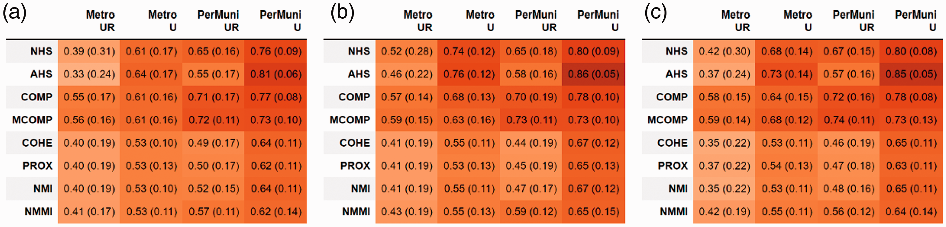
Stability (standard deviation) of all indices in different boundary settings. The gradient background color is based on the stability score ranging from 0 to 1, the darker the orange color is, the closer it is to 1. (a) All-day (b) work-hour and (c) home-hour.

Discussion

In this section, we explore some of the potential reasons behind the stability findings described in the previous section. Complementary analyses can be found in the Supplementary Materials.

Stability of hotspot scale indices (NHS and AHS) at the inter-city level

As explained in the previous section, hotspot scale indices (NHS and AHS) are more stable (less sensitive to methodological choices) when city boundaries are defined using only urban municipalities. We posit that this might be due to the fact that rural areas, which generally have smaller footfall, are dramatically changing the Lorenz curves and, as a result, the scale of the hotspots computed. We will now analyze in depth a few case examples that are representative of the global trends observed in our analyses. Figure 3(a) shows the Spearman correlation coefficients for the NHS index across all the combinations of spatial unit and interpolation methods per each of the four boundary settings. We can observe that combinations (G, Uni) and (G, Idw) are weakly or even not correlated with other methods in the Metro-UR causing the low stability score. Changing to other boundary settings, such as excluding the rural areas, all the coefficients involving methods (G, Uni) and (G, Idw) have a large increase and as a result NHS becomes more stable in Metro-U setting. Therefore, we will compare the NHS computed based on combinations (G, Idw) and (G, Pop) to explore what might cause the unstability or dissimilarity in the cities ranking.

Figure 3.

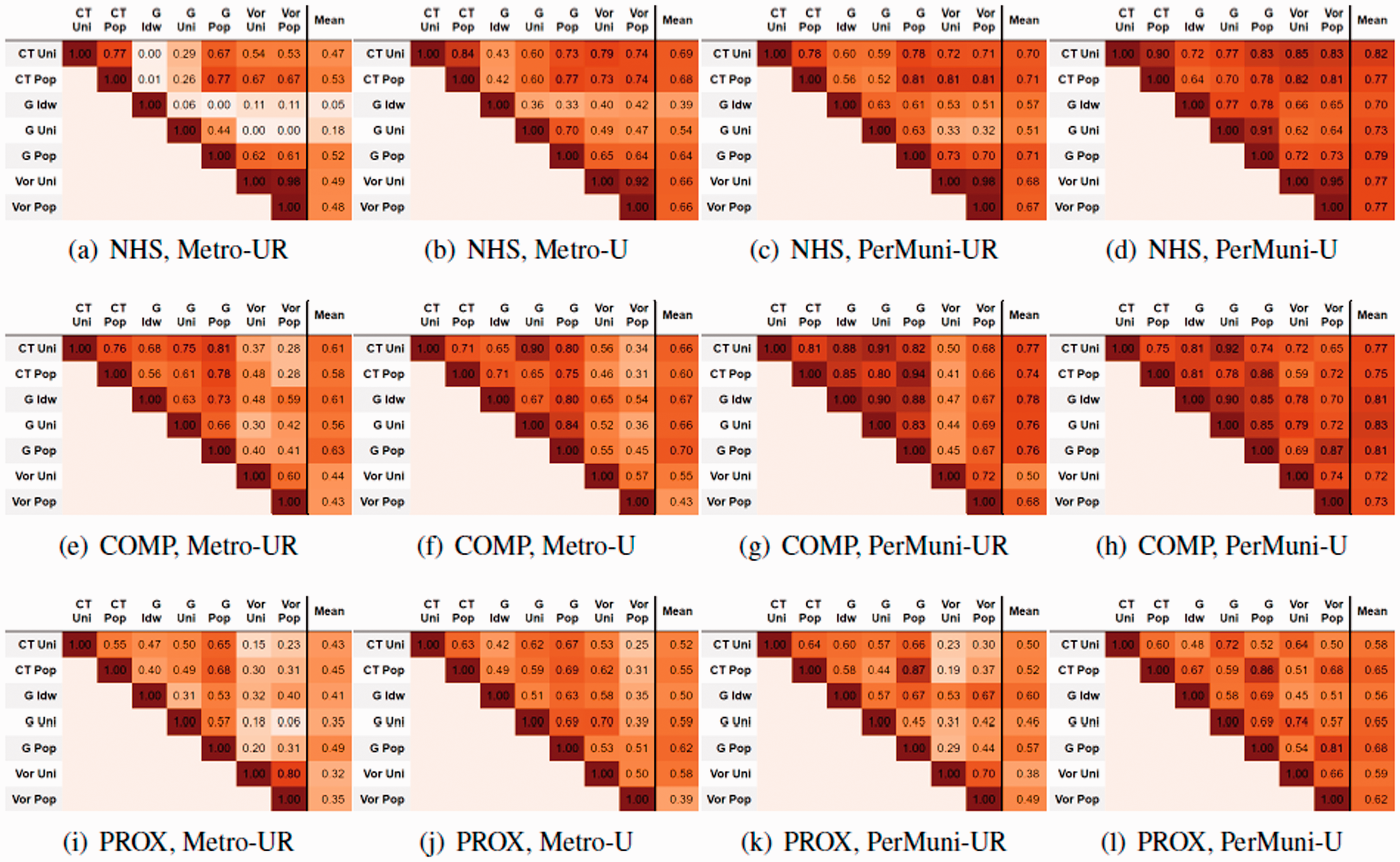
Spearman correlation coefficients $Coe f_{ind = NHS, b, j, k}$ (a–d), $Coe f_{ind = COMP, b, j, k}$ (e–h), and $Coe f_{ind = PROX, b, j, k}$ (i–l) between each pair of combinations (C_j,C_k) under four different boundary settings. The coefficient matrix is symmetric whose lower triangular part is omitted. (a) NHS, Metro-UR (b) NHS, Metro-U (c) NHS, PerMuni-UR (d) NHS, PerMuni-U, (e) COMP, Metro-UR (f) COMP, Metro-U (g) COMP, PerMuni-UR (h) COMP, PerMuni-U, (i) PROX, Metro-UR (j) PROX, Metro-U (k) PROX, PerMuni-UR and (l) PROX, PerMuni-U.

Figure 4(a) and (b) shows the comparison between Metro-UR and Metro-U settings for city 34 (Puebla-Tlaxcala) and city 39 (Rioverde-Ciudad Fernández). Each plot represents the Lorenz curve used to compute NHS _a based on a combination $C = (t, i)$ of type of spatial units t and interpolation method i in city a. We can observe that the more rural areas a city has, the more heavily the shape of Lorenz curve is changed by different combinations C, which causes variations in the number of hotspots identified. For example, Figure 4(a) shows that under the Metro-UR setting, NHS₃₄ = 200 and for NHS₃₉ = 34 based on the combination (G, Pop), which means that the ranking of city 34 is higher than city 39. Changing to the combination (G, Idw), NHS₃₄ decreases to 138 but NHS₃₉ increases to 466 reversing the rankings between city 34 and city 39 has reversed. This is caused by the fact that city 39 has more rural areas (99%) than city 34 (70%), and the Lorenz curve for city 39 is impacted more (much more closer to the diagonal) by changing from (G, Pop) to (G, Idw) than the curve for city 34.

Figure 4.

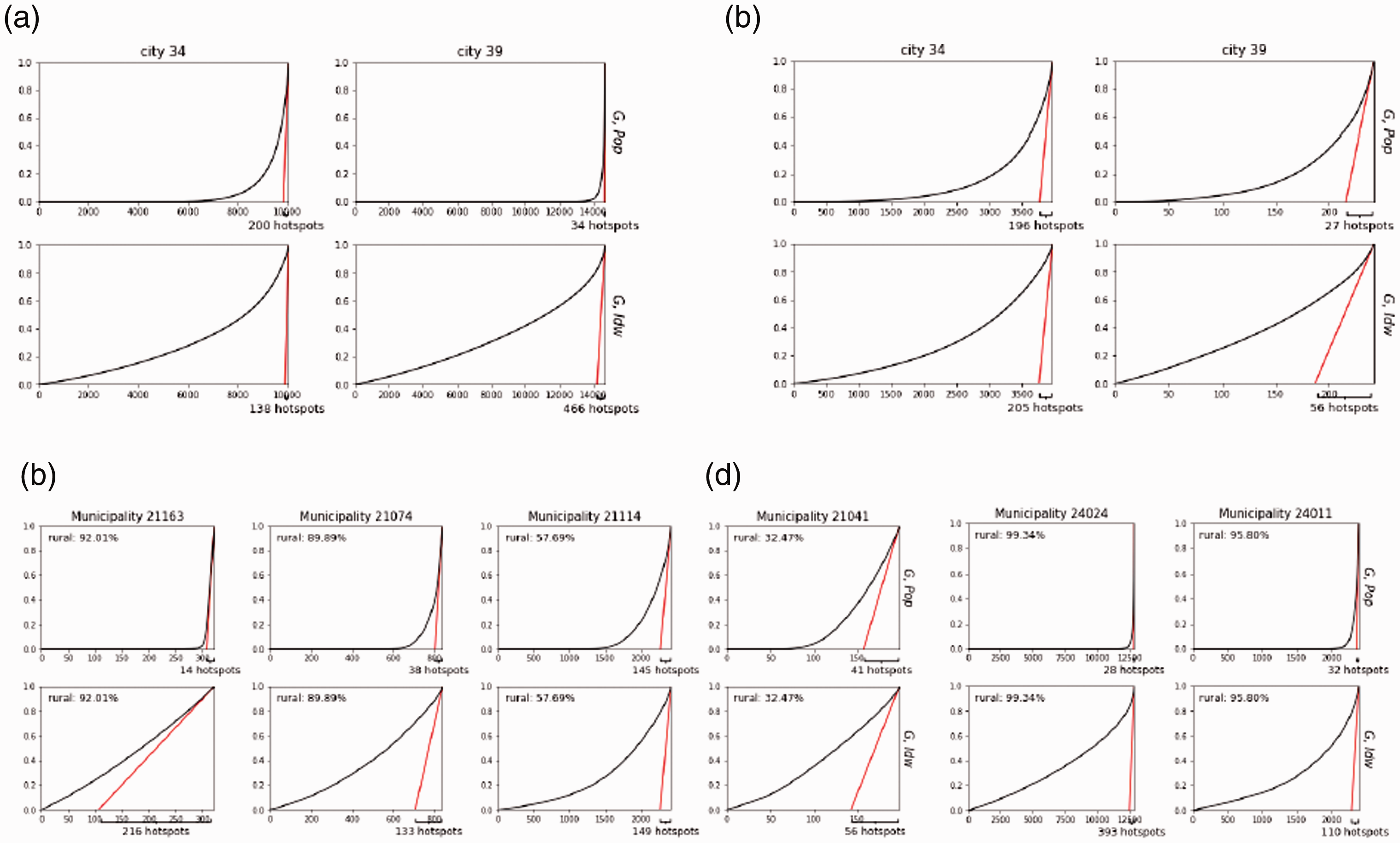
Lorenz curves for Loubar-based hotspots detection in city 34 and 39 in different boundary settings. The x-axis is rescaled to the number of spatial units to better explain the difference in NHS. Combination (G, Pop) and (G, Idw) are shown for comparison. City 34 has 70% of rural areas and 39 municipalities with various percentage of rural areas while city 39 has 99% of rural areas and 2 municipalities both with more than 95% of rural areas. (a) Metro-UR (b) Metro-U, (c) PerMuni-UR, municipaliites in city 34 and (d) PerMuni-UR, municipaliites in city 39.

On the other hand, the spatial units in the rural areas are not considered in the hotspot detection under the Metro-U setting. For example, the number of grids considered in city 39 in Metro-U setting is about 250, much smaller than in Metro-UR setting which is about 14,500. The impact brought by the variation in percentage of rural areas is mitigated by focusing on urban areas only in the Metro-U setting, i.e., the change in the Lorenz curve and the change in NHS from (G, Pop) to (G, Idw) is smaller and more consistent in both cities. When changing from (G, Pop) to (G, Idw), NHS₃₄ increases from 196 to 205 and NHS₃₉ increases from 27 to 56. Therefore, the ranking of both cities is better preserved by these two combinations.

Next, we shift our focus to the PerMuni-UR setting. In PerMuni-based settings, hotspots are detected per municipality. Therefore, the Lorenz curves might be affected by the percentage of rural areas in each municipality. City 34 as a whole metropolitan area has 70% rural areas, but it has 39 municipalities with various percentages of rural areas from 1% to 92%. Four example municipalities are shown in Figure 4(c). City 39 has two municipalities, both of which have similar percentages of rural areas as city 39 as a whole (Figure 4(d)). We observe that for municipalities with high percentage of rural areas, e.g., municipality $22163, 21074, 24024, and 24011$ , the Lorenz curves are heavily impacted by changing from (G, Pop) to (G, Idw). For municipalities with lower percentage of rural areas, e.g., municipality 21114 and 21041, the Lorenz curves are less impacted. As a result, changing from (G, Pop) to (G, Idw), the NHS₃₄ changes from 905 to 3663 and the NHS₃₉ changes from 60 to 503. Although city 34 still has a smaller change in NHS (increased 3 times) than city 39 (increased 7.4 times), the ranking between them is preserved. Therefore, the stability of NHS in Permuni-UR is better than in Metro-UR.

Stability of urban sprawl indices (COMP and MCOMP) at the inter-city level

As discussed in the previous section, urban sprawl indices computed with PerMuni-based boundary settings appear to be more stable than Metro-based ones (less sensitive to Metro-based choices). One of the possible reasons might be the different ways in which the population of a metropolitan area can be distributed across municipalities. For example, some metropolitan areas have a dominant urban core with the majority of human activities, while in other metropolitan areas there might be municipalities acting as sub-centers with similar levels of activity as their urban cores.

Take city 25 (Morelia) and city 46 (Tlaxcala-Apizaco) as examples (Figure 5). Both cities have multiple municipalities. But in city 25, the urban core is dominating, that is, the population of city 25 is mostly concentrated in one core urban region, e.g., (CT, Pop) and (Vor, Pop) in Metro-UR setting in Figure 5(a). While in city 46, the location of the hotspots varies. With the combination (CT, Pop) in Metro-UR, the permanent hotspots concentrate in the left-bottom corner (Figure 5(b)), just like city 25. But with the combination (Vor, Pop) in Metro-UR, permanent hotspots in other municipalities are detected thus increasing the value of the COMP index. As a result, since different metropolitan areas have different distributions of population over multiple municipalities, hotspots indices computed over metropolitan-based settings are not as stable. On the other hand, detecting hotspots in the municipality-based settings is more stable because the permanent hotspots are local to each municipality and overall the hotspots spread over multiple municipalities (see the second row in Figure 5(a) and 5(b)). And because COMP is normalized by the square-root of city’s geographical area, the distance between hotspots spreading over the city is normalized. Therefore, variances in the population distribution bring less instability to COMP indices across spatial units and interpolation methods.

Figure 5.

Permanent hotspots detected by combinations (CT, Uni) (Vor, Pop) for city 25 and 46. (a) City 25 and (b) city 46.

Rural areas also appear to play a role in index stability. Figure 3(e) to (h) shows the correlation coefficients for each pair of spatial unit and interpolation method combination across all boundary settings for the COMP index. We can observe that combinations (Vor, Uni) and (Vor, Pop) are the least correlated with other combinations, especially in settings including rural areas. When considering rural areas, the Voronoi polygons can cover large regions, e.g., the plot of (Vor, Pop) using the Metro-UR setting in Figure 5, as the cell towers tend to be sparse in rural areas. Since urban sprawl indices are computed based on the distance among centroids of polygons, these large Voronoi polygons drag the centroids away from dense population areas; and since the sizes of the Voronoi polygons are not homogeneous across different metropolitan areas, the inclusion of rural areas brings in high instability to hotspot urban sprawl indices. Finally, other minor discussion points can be found in the Supplemental Materials.

Conclusions

The rich spatio-temporal information provided by CDR data has provided great potential for studying human mobility dynamics in urban environments. A bulk of the literature has used CDR data to study the relationship between human dynamics—modeled through hotspot areas in cities—and various urban characteristics, such as spatial structure, transportation efficiency, and energy consumption. However, most of these studies are based on ad-hoc selections of city boundaries and spatial units.

In this paper, we provide a novel interpretable approach to carry out a systematic analysis of the stability of various hotspot indices in both static (inter-city) and dynamic (intra-city) settings. We have found that at the inter-city level, the urban municipality boundary is the best setting to obtain stable and robust city ranking results. Indices for scale of hotspots and degree of urban sprawl are strongly stable across all city boundary settings. Therefore, when a particular city boundary setting is desired, NHS, AHS, COMP, and MCOMP are good indices to work with. If the compactness of the family of indices (COHE, PROX, NMI, and NMMI) is of interest, it is better to use the municipalities with urban and rural areas (PerMuni-UR setting). If other city boundaries are required, we recommend using the (G, Pop) interpolating method as this method tends to be most correlated with other methods in all settings.

For intra-city level, the stability of indices is mostly weakly stable. Only the degree of urban sprawl (COMP and MCOMP) in Metro-based settings has moderate stability. The stability of indices in different cities has large variation, meaning some indices can be very strongly stable across interpolation methods in some cities but not stable at all in other cities. We have not found any index or boundary setting that would work well across cities. Thus, it is vital for researchers to use a consistent type of spatial units and interpolation methods across analyses.

This paper does not provide a comprehensive analysis of all the combinations of spatial units and interpolation methods that exist in the literature, but rather an analysis of the most common approaches currently used in the field. In addition, the analysis presented focuses only in one country. As future work, we will expand and generalize our spatial sensitivity analysis to more methodological choices, such as different grid sizes, or interpolation methods that consider terrain and land use patterns; and we will explore the applicability of our results to other countries.

Supplemental Material

sj-tex-1-epb-10.1177_2399808320985843 - Supplemental material for Spatial sensitivity analysis for urban hotspots using cell phone traces

Supplemental material, sj-tex-1-epb-10.1177_2399808320985843 for Spatial sensitivity analysis for urban hotspots using cell phone traces by Jiahui Wu, Enrique Frias-Martinez and Vanessa Frias-Martinez in EPB: Urban Analytics and City Science

Footnotes

Declaration of conflicting interests

The author(s) declared no potential conflicts of interest with respect to the research, authorship, and/or publication of this article.

Funding

The author(s) disclosed receipt of the following financial support for the research, authorship, and/or publication of this article: This work was supported by the U.S. National Science Foundation [grant number 1750102].

ORCID iDs

Jiahui Wu

Enrique Frias-Martinez

Supplemental material

Supplemental material for this article is available online.

Jiahui Wu is a doctoral candidate in the College of Information Studies at University of Maryland. He received his Master degree in Information Science from Peking University and Bachelor degree in Information Management and Information System from Sun Yat-sen University. His research interests include urban computing, spatio-temporal behavior modeling, machine learning and data visualization.

Enrique Frias-Martinez is a scientific researcher in Telefonica Research, Madrid, Spain. His research areas focus on urban computing, mobility, and big data for social good. Before joining Telefonica, he was a researcher for the Department of Biomedical Engineering of the University of California, Los Angeles, for the Department of Information Systems and Computing of Brunel University (London) and for the Courant Institute of Mathematical Sciences, New York University. Enrique received his PhD in Computer Science from the Universidad Politécnica de Madrid (Spain) in 2002, where he was awarded the Best PhD Thesis Award of the School of Computer Science.

Vanessa Frias-Martinez is an assistant professor in the iSchool and UMIACS, and an affiliate assistant professor in the Department of Computer Science at the University of Maryland, College Park. Frias-Martinez’s research areas are data-driven behavioral modeling and spatio-temporal data mining. Her research focuses on the use of large-scale ubiquitous data to model the interplay between human mobility and the built environment. Specifically, she develops methods to model and predict human behaviors in different contexts and creates tools to aid decision makers in areas such as disaster preparedness and response or urban planning. Her research is funded by the NSF, including a CAREER Award, and by the World Bank. Frias-Martinez received her PhD in Computer Science from Columbia University.

References

Ahas

Aasa

Yuan

, et al. (2015) Everyday space–time geographies: Using mobile phone-based sensor data to monitor urban activity in Harbin, Paris, and Tallinn. International Journal of Geographical Information Science 29(11): 2017–2039.

Angel

Parent

Civco

(2010) Ten compactness properties of circles: Measuring shape in geography. The Canadian Geographer/Le Géographe Canadien 54(4): 441–461.

Bachir

Gauthier

Yacoubi

, et al. (2017) Using mobile phone data analysis for the estimation of daily urban dynamics. In: 2017 IEEE 20th international conference on intelligent transportation systems (ITSC). Piscataway, NJ: IEEE, pp. 626–632.

Bogomolov

Lepri

Staiano

, et al. (2015) Moves on the street: Classifying crime hotspots using aggregated anonymized data on people dynamics. Big Data 3(3): 148–158.

Chen

Pei

Shaw

, et al. (2018) Fine-grained prediction of urban population using mobile phone location data. International Journal of Geographical Information Science 32(9): 1770–1786.

Chen

Arribas-Bel

Singleton

(2019) Understanding the dynamics of urban areas of interest through volunteered geographic information. Journal of Geographical Systems 21(1): 89–109.

CONAPO (2015) Delimitación de zonas metropolitanas. Available at: www.conapo.gob.mx/es/CONAPO/Datos_Abiertos_Delimitacion_de_Zonas_Metropolitanas (accessed 17 January 2020).

Demographia (2020) Definition of urban terms. Available at: http://demographia.com/db-define.pdf (accessed 17 January 2020).

Deville

Linard

Martin

, et al. (2014) Dynamic population mapping using mobile phone data. Proceedings of the National Academy of Sciences of the United States of America 111(45): 15888–15893.

10.

Doyle

Hung

Farrell

, et al. (2014) Population mobility dynamics estimated from mobile telephony data. Journal of Urban Technology 21(2): 109–132.

11.

Ewing

, (2008) Characteristics, causes, and effects of sprawl: A literature review. In: Marzluff JM, Shulenberger E, Endlicher W, et al. (eds.) Urban Ecology: An International Perspective on the Interaction between Humans and Nature. Boston, MA: Springer US, pp. 519–535.

12.

Gariazzo

Pelliccioni

Bogliolo

(2019) Spatiotemporal analysis of urban mobility using aggregate mobile phone derived presence and demographic data: A case study in the city of Rome, Italy. Data 4(1): 8.

13.

Ghahramani

Zhou

Hon

(2018) Mobile phone data analysis: A spatial exploration toward hotspot detection. IEEE Transactions on Automation Science and Engineering 16(1): 351–362.

14.

Hoteit

Secci

Sobolevsky

, et al. (2014) Estimating human trajectories and hotspots through mobile phone data. Computer Networks 64: 296–307.

15.

Huang

Sellers

(2007) A global comparative analysis of urban form: Applying spatial metrics and remote sensing. Landscape and Urban Planning 82(4): 184–197.

16.

INEGI (2010) Colección: Cartografía geoestadística urbana, cierre del censo de población y vivienda 2010. Available at: www.inegi.org.mx/app/mapas/?t=0710000000000000&tg=3604 (accessed 17 January 2020).

17.

Isaacman

Becker

Cáceres

, et al. (2012) Human mobility modeling at metropolitan scales. In: Proceedings of the 10th International Conference on Mobile Systems, Applications, and Services, MobiSys ’12. New York, NY: ACM, pp. 239–252.

18.

Kang

Liu

, et al. (2012) Towards estimating urban population distributions from mobile call data. Journal of Urban Technology 19(4): 3–21.

19.

Kubíček

Konečný

Stachoň

, et al. Š (2019) Population distribution modelling at fine spatio-temporal scale based on mobile phone data. International Journal of Digital Earth 12(11): 1319–1340.

20.

L3 Harris (n.d) Hotspot analysis. Available at: www.harrisgeospatial.com/docs/hotspotanalysis.html (accessed 8 August 2020).

21.

Le Néchet

(2012) Urban spatial structure, daily mobility and energy consumption: A study of 34 European cities. Cybergeo. 580: 1–30.

22.

Louail

Lenormand

Cantu Ros

, et al. (2014) From mobile phone data to the spatial structure of cities. Scientific Reports 4: 5276.

23.

Ouředníček

Nemeškal

Špačková

, et al. (2018) A synthetic approach to the delimitation of the Prague metropolitan area. Journal of Maps 14(1): 26–33.

24.

Peredo

García

Stuven

Ortiz

(2017) Urban dynamic estimation using mobile phone logs and locally varying anisotropy. In: Gómez-Hernández JJ, Rodrigo-Ilarri J, Rodrigo-Clavero ME, et al. (eds.) Geostatistics Valencia (2016). Cham: Springer International Publishing, pp. 949–964.

25.

Ratti

Frenchman

Pulselli

, et al. (2006) Mobile landscapes: Using location data from cell phones for urban analysis. Environment and Planning B: Planning and Design 33(5): 727–748.

26.

Reades

Calabrese

Sevtsuk

, et al. (2007) Cellular census: Explorations in urban data collection. IEEE Pervasive Computing 6(3): 30–38.

27.

Schwanen

Dieleman

Dijst

(2001) Travel behaviour in Dutch monocentric and policentric urban systems. Journal of Transport Geography 9(3): 173–186.

28.

Statstutor (2020) Spearman’s correlation. Available at: www.statstutor.ac.uk/resources/uploaded/spearmans.pdf (accessed 17 January 2020).

29.

Traunmueller

Quattrone

Capra

(2014) Mining mobile phone data to investigate urban crime theories at scale. In: International Conference on Social Informatics. Switzerland: Springer, pp. 396–411.

30.

Vieira

Frias-Martinez

Oliver

, et al. (2010) Characterizing dense urban areas from mobile phone-call data: Discovery and social dynamics. In: 2010 IEEE Second International Conference on Social Computing. Piscataway, NJ: IEEE, pp.241–248.

31.

Wassmer

(2000) Urban sprawl in a us metropolitan area: Ways to measure and a comparison of the Sacramento area to similar metropolitan areas in California and the us. CSUS Public Policy and Administration Working Paper (2000–2003).

32.

Chen

Frias-Martinez

, et al. (2019) The inverted u-shaped effect of urban hotspots spatial compactness on urban economic growth. Royal Society Open Science 6(11): 181640.

33.

Zuo

Zhang

(2012) Detection and analysis of urban area hotspots based on cell phone traffic. Journal of Computers 7(7): 1753–1760.

Supplementary Material

Please find the following supplemental material available below.

For Open Access articles published under a Creative Commons License, all supplemental material carries the same license as the article it is associated with.

For non-Open Access articles published, all supplemental material carries a non-exclusive license, and permission requests for re-use of supplemental material or any part of supplemental material shall be sent directly to the copyright owner as specified in the copyright notice associated with the article.

0.00 MB

0.26 MB

0.03 MB