New algorithms for generating isovist field and isovist measurements

Abstract

Isovist fields are powerful tools for expressing and analyzing spatial configurations. There is also useful software that allows one to calculate the isovist field variables. However, the complexity and the speed of the isovist field production algorithms have limited the diverse uses of isovist fields as a spatial configuration expressive model. In this paper, we present an algorithm for generating the isovist field which is simpler than the rivals. This algorithm relies on calculating the isovist for the corner points before generating the isovist fields. A complementary algorithm is also proposed which quickly updates isovist field calculations after limited changes in the environment take place. The speeds of these two algorithms are also checked here in real cases and are compared to the well-known fast algorithms. In addition, more efficient methods are proposed to calculate variables related to distance-to-the-walls metrics within an isovist. This method, which is fast and accurate, uses slices of isovist as a base to calculate these variables with the help of integral calculations. We hope these methods accelerate the evolution of isovist field models and help make algorithmic design based on isovist fields a more convenient technique.

Keywords

Spatial configuration expressive models isovist field generation isovist measurements

Introduction

Background

Introduction to spatial configuration expressive models

In architecture as a science, it is necessary to define a theory that expresses the effect of spatial configuration on human perception and behavior. To achieve this goal, some researchers have tried to suggest mathematical models as suitable quantifications of spatial configurations. These mathematical models could be called “Spatial configuration expressive models.”

An ideal spatial configuration model should have two characteristics. On the one hand, it should include data on the most important aspects of the space configuration that affects human perception and behavior. On the other hand, the model should be simple enough to be produced and used in research and applied design. Among spatial configuration expression models, the models based on visibility data of the environment have attracted the attention of researchers because of their great potentialities.

Visibility-based spatial configuration expressive models

Everything exists or happens in space, and space can be considered as the container of everything. From this viewpoint, spatial configuration can be considered a law that governs whatever one can see at any given moment and has access to, if they move. Theories, such as refuge and perspective (Appleton, 1996; Hildebrand, 1999), even try to define the two factors of visual and access data, as the main bases for human perception and behavior in the environment.

According to this logic, if spatial configuration is translated into a simpler data structure that includes visual and access data of each point of the environment, the structure will include the most important aspects of the spatial configuration that affects human perception and behavior. Some researchers have tried to build such spatial configuration expressive models based on whatever one can see or has access to in each position. For the sake of convenience, we will refer to these models as visibility models or simply models. Over time, various models have been proposed for environmental analysis. Some of the most famous models are Visibility Graph Analysis (VGA) and isovist fields (Batty, 2001; Turner, 2001).

For generating a model to hold visibility information of the environment with respect to practicality, as the second important quality of the models, a set of sample points should be selected to present all points of the environment. To simplify the visual and access data of a given position, the environment is usually simplified to a horizontal section (plan) of itself. In the next step, the visual and access data of every selected sample point in the environment will be calculated (Figure 1).

Figure 1.

Steps of generating a visibility model: A. The environment is simplified into two dimensions. B. A set of sample points are selected from the environment. C. The visual and access data of every sample point are extracted.

Different methods of translating and storing visibility data of the environment in sample points result in different visibility models. Three slightly different and currently popular visibility models are isovist field, Visibility Graph Analysis (VGA), and Radial Array.

Isovists are the tools to store visual data of a point. Benedikt (1979) defined an isovist as “the set of all points visible from a single vantage point in space with respect to an environment” and claimed that measurements of this shape are related to the perceived quality of space. In a simplified environment used for generating the models, an isovist is a polygon. This polygon shape holds the visual and access data of its vantage point (Batty, 2001).

VGA stores the visual and access data in the form of a comprehensive visual graph, with sample points as its vertices. The Radial Array stores visual and access data at each sample point in a collection of rays to the surrounding walls. Because all of these models, that is, VGA, isovist field, and Radial Arrays, are built to hold visual and access data, it is usually possible to translate one model measurements to fit another. Therefore, each of the models can be used interchangeably. The most important difference between these models is that the isovist fields have more information about the environment than the other two models which can be considered as a simplified version of the isovist field. Yet, the isovist field usually requires an additional measurement and simplification step after production for statistical use.

Available algorithms for generating models

Generating visibility models is not an easy task and must be done by computer software. None of the mentioned models are completely accurate because firstly, they simplify the environment, and secondly, they use a selected set of sample points instead of all possible positions of the environment. As the number of sample points increases, the accuracy of the measurements increases as well, though generating the model will take more time. But the time available to researchers is limited, so there must always be a balance between the accuracy of a model and the time it takes to generate the model. The speed of creating a model is, therefore, an important factor.

Algorithms are the core of any software that generates models, and they are the most important factor that determine their speed. One of the well-known algorithms for calculating the isovist polygon was proposed by Davis and Benedikt (1979). This algorithm was very simple, but not fast enough. In 1985, Asano introduced a new and fast algorithm to create an isovist shape in the environment. In 1995, Heffernan and Mitchell proposed a faster algorithm with similar capabilities which was evaluated as very complex (Heffernan and Mitchell, 1995). Later in 2014, Bungiu et al. proposed an algorithm which was claimed to be faster than the Asano algorithm in many cases.

The algorithms mentioned so far are employed for generating a single isovist, and each can be used many times. However, there are other algorithms for generating VGA and Radial Array that are slower and simpler than most of these algorithms. It is also possible to suggest ways to improve the generation speed of a model, such as using parallel computing which usually leads to an increase in complexity.

Software available for generating visibility models:

There is a number of software available and usable for different types of visibility model research which are as follows:

Depthmap and DepthmapX, as two free-to-use software, were developed at University College London by Turner (2004) and others. They offer VGA models and measurements, and it takes a few seconds to create a medium-sized model by them. They are available to researchers at UCL official site.

Another software, Syntax 2D, was developed at the University of Michigan by Wineman et al. (2007) is able to generate both VGA and isovist fields and even more models. This software is open source and can be further developed, but unfortunately, the algorithms used are not fast enough and the total speed of the software is not efficient.

Isovist-App, a more recent and powerful software, provided by Benedikt and McElhinney (2019), is available on isovists.org. This software is also updated at times and can be improved over time. It uses better algorithms and also complex techniques such as using graphic processor powers which improve its calculation speed. It seems that this software uses techniques to increase the visual quality of the provided images based on suggested ways of Psarra and McElhinney (2014), without increasing the accuracy of the actual model. As a result, it is able to provide high-resolution images of the results with high speed, and it can try to increase its models and image accuracy over time. The software uses several algorithms for calculation, including a version of Asana and Radial Array. It also uses some “stochastically selected locations” algorithm for calculating other measurements such as visibility, control, and controllability. The software also uses different versions of “visibility flooding” algorithms in generating global measurements, such as metric, visual, and angular depth (McElhinney, 2020).

In recent years, some researchers have attempted to use algorithmic designs based on visual data from the environment. Some also tried to provide software for this purpose, but the software was usually too complex, with a limited scope of use (Schneider and Koenig, 2012).

Contribution

Creating a model for expressing spatial configuration based on isovist measurements is a promising approach, but the current tools are far from ideal. More research and development is needed for these models to be useful in predicting human perception and behavior in relation with the environment. Researchers are trying to improve these models by proposing changes to them and their measurements. Unfortunately, these efforts have faced two major challenges.

Firstly, generating isovist models requires software to be open source and easy to understand and modify, while the current fast and practical software is not so. Developing new software for a new model can be problematic because the known fast algorithms are also complex which discourages researchers in modifying the current models.

Secondly, any newly defined measurement can be useful, only if its relationship to human perception and behavior is well determined. Defining such relationships usually requires multiple experiments as well as the measurement of human perception and behavior in different environments. After all these efforts are made, due to the presence of intervening variables, what one can define is only a correlation between measurement and perception. The only way to prove the causality of a measurement on perception is to change the proposed measurement and to observe a subsequent change in perception. To do this methodically, one would need an algorithmic design software for designing and modifying the environment in order to change certain measurements in a specific direction. Unfortunately, as far as we know, there is no such suitable software.

As for the first problem, in the Introducing a New Algorithm for Generating Isovist Fields to Be Fast and Simple section, we will present an algorithm for generating isovist models that is simple to grasp and implement with lower time complexity. For the second problem, in the an Algorithm for Updating Models After Limited Changes section, we will present an algorithm that allows for updating isovist models after changes in the environment so that the run time will depend on the extent of the changes. Furthermore, in the section a New Method for Calculating the Distance from Wall Measurements, we present an algorithm for efficient and accurate calculation of distance from wall measurements. Besides these theoretical results, we present open-source software that implements these improvements and is capable of designing algorithms based on isovist characteristics. We hope our proposed software is a great help to researchers. The section Characteristics of the Proposed Solutions contains an analysis of the run time and memory usage of our algorithms, providing both theoretical bounds and evidence from simulation. Finally, we will conclude with a review and discussion in the Discussion section.

Defining the proposed solutions

Introducing a new algorithm for generating isovist fields to be fast and simple

Introduction of new terms used in the proposed algorithm

Some of the terms used in the proposed algorithms are as follows:

Walls and corner points: Each environment consists of straight-line walls that intersect only at the end points, called corner points. Each wall has two corner points, and each corner point has one or two walls.

Sample point: As one of the selected points in the environment to check for isovist measurement, these points exist as a grid in the environment.

Visual arrow: The visual arrow is a special imaginary structure of the proposed algorithm with three components (arrow shapes in Figure 2, steps 2-1 and 2-2). The first component can be a sample point or a corner point, considered as the starting point of the arrow. The second component is a corner point, which is considered as the endpoint of an arrow and can be seen from the first component. The third component is a position on the perimeter wall. This position is calculated, if possible, by extending the arrow until it hits the wall. Note that it is not possible at times to extend the arrow. In such cases, the final position will be the same as the corner point.

Figure 2.

The steps of the proposed main algorithm for generating isovist fields.

Visual arrows have an angle value which is the angle between the arrow and the positive direction of the X-axis. Visual arrows can be labeled as neutral, positive, or negative. A visual arrow is neutral if the walls of the corner point are on two different sides of the arrow. This is true where the arrow expansion is impossible. A visual arrow is positive if the walls of the corner point are on the clockwise side of the arrow. And it is labeled negative if the walls of the corner point are on the counterclockwise sides of the arrow. Note that after finding all the visual arrows for a sample point, creating the isovist polygon is a matter of connecting visual arrows in angular order (Figure 2, steps 2-2 and step 2-3). A visual arrow label is used to specify whether the second component or the third component should be used in generating the connection with the next visual arrow.

Slices and the sliced isovist: Isovist polygons may be angularly divided into parts, which can see different boundary lines of the polygon of the isovist (Figure 2, steps 1-1 and step 2-3). Each part is a triangle called an isovist slice. A slice has two visual arrows and a part of the wall as its borderline. Any isovist polygon could be considered a sorted set of slices. This set is called a sliced isovist which is a way to present the isovist polygon. Most polygon measurements can be calculated by extracting similar measurements from the slices.

Radial List Algorithm: This is a simple algorithm for creating a new isovist in the environment or updating part of an existing one. This type of algorithm is basically like an Asano (1985) algorithm, but without the AVL tree. It is not as fast as the Asano algorithm, but it is much simpler and can be recommended because of its simplicity. The steps of this algorithm are as follows:

1. Arrange all the corners around the center of the isovist angularly.

2. Throw a ray from a selected starting direction into the environment and store all the walls intersecting with this ray.

3. Find in the stored walls the nearest wall to the center and label it.

4. Rotate the ray and at every corner point met by the ray, do as follows:

4.1. Add or remove walls of the corner point from stored walls in a way that the walls intersecting with the ray become updated.

4.2. If a wall is added, check it with the nearest existing wall and, if necessary, label it as the nearest wall.

4.3. If the nearest wall is removed, search among the stored walls and find the nearest new wall and label it.

4.4. If the nearest wall undergoes any change, create a visual arrow at that point and create an isovist slice with the previous visual arrow.

5. When the ray rotation is finished, the set of the produced slices is the sliced isovist.

A main algorithm in detail

The steps of the proposed algorithm are as follows (Figure 2):

0. Build the environment and consider sample points in grid shape with specific intervals. For any sample point, consider an empty pool (list) for storing visual arrows.

1. For every corner point of the environment, do as the following:

1.1. Generate the isovist polygon of the corner point with any known algorithm. For simplicity, Radial List Algorithm is suggested.

1.2. Use a sweep with basic scan-fill algorithm (foley et al., 1996, pp. 92–99; Scholar.cu.edu.eg, 2020) to find all sample points that are included in that isovist polygon.

1.3. For all such sample points, build a neutral visual arrow with the sample point and the corner point. Add the generated visual arrow to the sample point pool.

2. For every sample point of the environment, the following procedure should be followed:

2.1. Sort all visual arrows according to their angle value in the pool of the sample points.

2.2. Now every couple of adjacent visual arrows of the pool builds a slice of the sliced isovist of the sample point through the following steps:

2.2.1. If the first visual arrow is negative, consider the position of the second component of this visual arrow. Otherwise, consider the third component position.

2.2.2. If the second visual arrow is positive, consider the position of the second component of this visual arrow. Otherwise, consider the third component position.

2.2.3. Connect two considered points and generate a slice with the sample point as the third corner of the triangle.

2.3. All generated slices together form the isovist of the sample point. Do the measurements for the isovist of the sample point with the help of these slices.

An algorithm for updating models after limited changes

In algorithmic designs, minor changes in the environment occur much often, so it is important to be able to update quickly and efficiently the generated model and its measurements after minor changes. We propose here a secondary algorithm for updating the model and the measurements provided by the main proposed algorithm. This algorithm updates visual arrows and databases and could be used many times to update models continuously during the designing process. However, it should be noted that if the number of the changes in the environment are too many, the usefulness of this algorithm will be limited.

In this algorithm, three tags (old, removal, and add-on) are provided for visual arrows. Old visual arrows are created before the current change in the previous steps. Removal visual arrows are those which are not valid in the changed environment and are created to clear obsolete old visual arrows. Add-on visual arrows are the ones which are added in this step.

Changes in the environment can be done by deleting certain parts and adding some other ones, and this can be translated into removing and adding walls and corner points. Adding and deleting corner points cause changes to the visual arrows of the environment. The changes could be grouped as follows:

1. Deleting some corner points makes some visual arrows invalid because their second components are deleted.

2. Adding some corners requires new visual arrows for sample points that are in the visible area of the added corner point.

3. Deleting and adding lines necessitate updates for some visual arrows because their third component (the final point) is changed.

As for group A, it is sufficient to use step 1 of the main algorithm in deleting corner points before issuing any changes and to generate visual arrows with the tag Removal. Later, these visual arrows will be used to remove invalid old visual ones.

Concerning group B, it is enough to use step 1 of the main algorithm as for the added corner point and generate visual arrows with the tag Add-on.

Addressing group C is more complex and requires the following steps to be done for each corner point:

1. Tag slices that might change for each corner point, before issuing the changes. All slices that change should be tagged, but it is not harmful if unnecessary slices are also labeled. It only slows down the algorithm. The easiest way to do this is to tag the slices that are in the same direction of the corner points which were changed, given the angles of the corner points.

2. Consider the corner point as the center of the symmetry within isovist. Also, tag all the slices that can somehow mirror any slice tagged in the previous step.

3. In the corner point, first generate visual arrows with the removal tag by using steps 1–2 and 1–3 only for tagged slices. Unchanged slices should be used.

4. Then the isovist shape of the corner point should be updated only in the tagged slices. Almost all methods of isovist generation can update only a specific part of the isovist. For simplicity, using the Radial List algorithm is suggested. Then generate visual arrows with the tag add-on for the new slices by using 1-2 and 1-3 steps of the main algorithm.

After these steps are taken, visual arrows with the tags add-on or removal are added to some of the sample points. The isovist of these sample points should be updated as follows:

1. Sort the visual arrows angularly.

2. First remove each visual arrow with the tag removal, along with every old visual arrow that the second component (corner point) of it is the same as the second component of the removal visual arrow.

3. Change all visual arrows with the tag add-on to the tag old (for future changes).

4. Generate the isovist of the sample point as in step 3 of the main algorithm.

A new method for calculating the distance from wall measurements

In our proposed algorithm, the isovist polygons are defined as a sorted set of slices. Some measurements of the isovist could be defined as the statistical calculations of the same measurements of the slices. For example, the area of an isovist is the sum of its slice areas and the drift of an isovist is the sum of the drifts of slices divided by the areas of the same slices.

However, calculating the distance from the walls is not an easy job. Measuring the distance from the walls is important because it is one of the few measurements which are promising in determining the quality of the space. As Ostwald and Davos (2020) point out, calculating the distance from the walls is assumed to be possible only with the help of the Radial Array algorithm. This algorithm sends several rays to the environment and considers the distance of the center from the point where the rays hit the wall. To do this for the proposed algorithm, the simplest idea was to throw the rays at the boundary lines within the calculated isovist. Because the slices are arranged angularly, this can be done with O (1) for each ray and O (ray number) for the isovist shape.

It should be noted that isovist polygons can be highly irregular. This indicates that if the number of the rays is limited, the accuracy of the results may be significantly reduced, and if the number of the rays is large, the calculation time will be increased.

There is no better way as long as radiation is used, so we have suggested another method in our proposed algorithm. In the isovist created by the proposed algorithm, the field of view is divided into several slices, and the end boundary of each slice is a straight line. The distance from the wall in each of these slices is a continuous mathematical function, and therefore, in a slice distance from the wall, it can be calculated with a single integral formula. For the whole isovist, it is sufficient to use statistical tools to calculate the sum of the distances from the walls in the slices (Figure 3).

Figure 3.

Up: For statistical measurements in the radial algorithm, radial length is considered as a discontinuous function which shows the distance from the walls. Down: In the proposed method, distance from the wall is considered a continuous function. Right: In a triangle, distance from the wall could be calculated as D = $f (x) = ((d \times \sin (α)) \div s i n (π - α - x))$ .

To go into detail, in the i-th triangle of the isovist, the distance from a corner could be defined as D = $f i (x) = (d i \times \sin (α i) \div \sin (π - α i - x))$ . Based on this function, statistical measurements of the distance from the wall in a single triangle could be calculated. Accordingly, the mean distance from the wall in a triangle of an isovist is equal to $M i = \frac{1}{θ} \times (\int^{} f i (θ) - \int^{} f i (0))$ .

And also the mean distance from the wall in the whole isovist is equal to M = $\frac{1}{2 π} \times \sum^{} m e a n d i s t a n c e f r o m t h e w a l l i n i - t h t r i a n g l e * v i s u a l a n g l e o f i - t h t r i a n g l e$ =

\frac{1}{2 π} \times \sum_{i} M i \times θ i = \frac{1}{2 π} \times \sum_{i} \int^{​} (f i (θ) - \int^{​} f i (0)) .

Also if it is considered that $g i (x) = {(f i (x) - M)}^{2}$ and $h i (x) = {(f i (x) - M)}^{3}$ and $J i (x) = {(f i (x) - M)}^{4}$ , then:

V = variance of distance from the wall in an isovist = $\frac{1}{2 π} \times \sum_{i} (\int^{} g i (θ) - \int^{} g i (0))$ .

Sd = standard deviation from the wall in an isovist = $\sqrt{V}$ .

S = skewness of distance from the wall in an isovist = $\frac{1}{2 π \times S d} \times \sum_{i} (\int^{} h i (θ) - \int^{} h i (0))$ .

K = kurtosis of distance from the wall in an isovist = $\frac{1}{2 π \times S d} \times \sum_{i} (\int^{} J i (θ) - \int^{} J i (0))$ .

Solutions to $\int^{} f i (θ)$ , $\int^{} g i (θ)$ , $\int^{} h i (θ)$ , and $\int^{} J i (θ)$ could be found in part 1 of the supplementary materials (solutions for the integral calculations used in distance from the wall measurements).

To put these calculations into practice, first, the mean distance from the wall in each triangle of the isovist should be calculated, which is done by solving an equation that is not very simple. Then M, the mean distance from the wall in the whole isovist, should be calculated using the results for each triangle. In the next step, the variance, skewness, and kurtosis of each triangle should be calculated by the help of M. Finally, using the variance, skewness, and kurtosis of each triangle, the statistical measurements for the whole isovist can be calculated.

Characteristics of the proposed solutions

The speed of two proposed algorithms in practice

It is ideal to compare the speed of any proposed new algorithm with those of its rivals in real-world scenarios. But to compare their speed in real cases, it is necessary to set a standard for accuracy which is quite complex. Unfortunately, rival software is not fully documented or open source. Therefore, we compare the proposed algorithm with the two well-known Asano and Bungiu algorithms in terms of model production speed (Figure 4). The results are shown in Table 1.

Figure 4.

Environments used to test the speed of the proposed algorithm. Left: sample A and Right: sample B.

Table 1.

Test results. Time consumption (in seconds) for each action of the conducted experiment.

Number of sample points used in the experiment	212K, s	53K, s	13K, s
Calculating the isovist of the sample points with the Asano algorithm without doing measurements for sample A.	553.5	135.2	34.7
Calculating the isovist of the sample points with the Bungiu algorithm without doing measurements for sample A.	77.6	18.9	4.8
Calculating the isovists of the sample points with the proposed algorithm without doing measurements for sample A.	18.2	6.1	2.2
Calculating the isovist of the sample points with the Bungiu algorithm without doing measurements for sample B.	244.2	59.4	15.1
Calculating the isovists of the sample points with the proposed algorithm without doing measurements for sample B.	78.8	29.3	13.3
Calculating the isovists of the sample points with the proposed algorithm plus doing the measurements for sample A.	22.9	7.7	2.5
Updating the isovists and the measurements after changing 9 shapes of sample A.	11.6	4.4	1.2
Updating the isovists and the measurements after changing 5 shapes of sample B.	26.1	9.9	2.9
Updating the isovists and the measurements after changing a single shape of sample A.	5.1	1.01	0.36

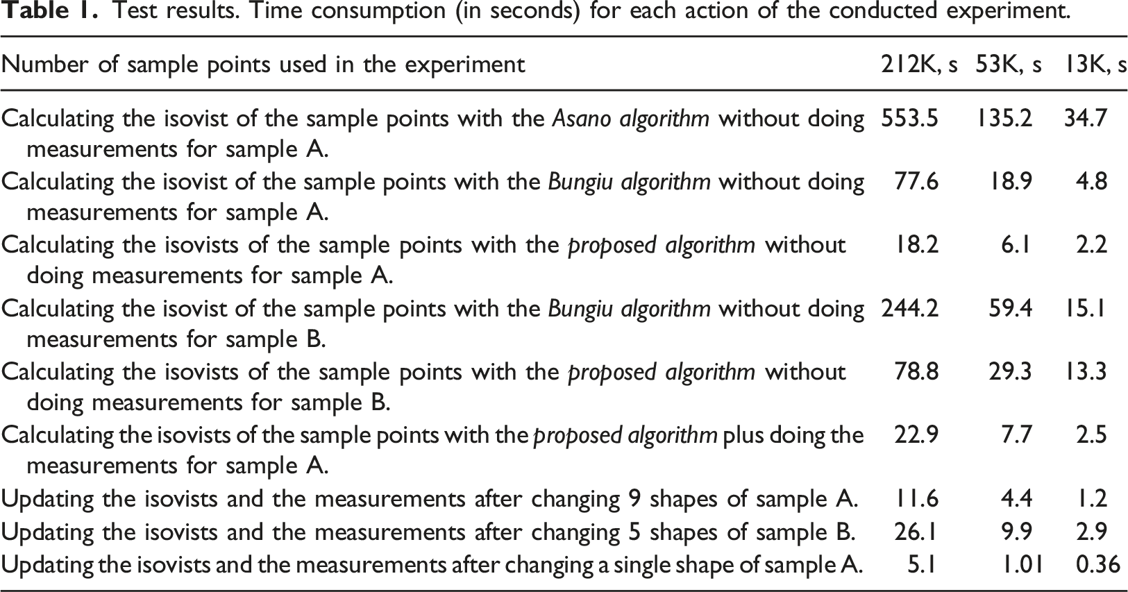
The results show that, to create an isovist field, the proposed algorithm is faster than Asano or Bungiu algorithms. The speed of updating the isovist’s data and recalculating the measurements after making changes is also much faster than generating a model from scratch with our proposed algorithm. But, it is noteworthy that the speed of the secondary proposed algorithm is greatly affected by the extent of changes in the environment. This makes this algorithm suitable for algorithmic designs because the intended changes in algorithmic designs are not often extensive. It is also notable that because of high volume of pre-calculation, the rate of time consumption of proposed algorithm increases slower that other algorithm when number of sample point increases.

To create an isovist field, we need to determine which points are in the open part of the environment and which points are in opaque shapes. This may take much time by simple algorithms. In our experiment, if a beam is fired from any sample point and the number of intersections of the beam with the walls is counted, it takes about 51 s for 53,000 sample points to determine which sample points are in the open part. This checking can be done faster by using smart ideas such as translating the environment into a quadtree which increases complexity of the whole process. Note that the time here does not include the time consumption listed in Table 1 for the Asano and Bungiu algorithms.

The proposed algorithm makes this step completely unnecessary because sample points that are not in the open part could not see any corner point, so they have no visual arrows. After updating the isovist database and the measurements with the secondary algorithm, it automatically remains true that any sample point without a visual arrow is not in the open part and should not be calculated in the final measurements.

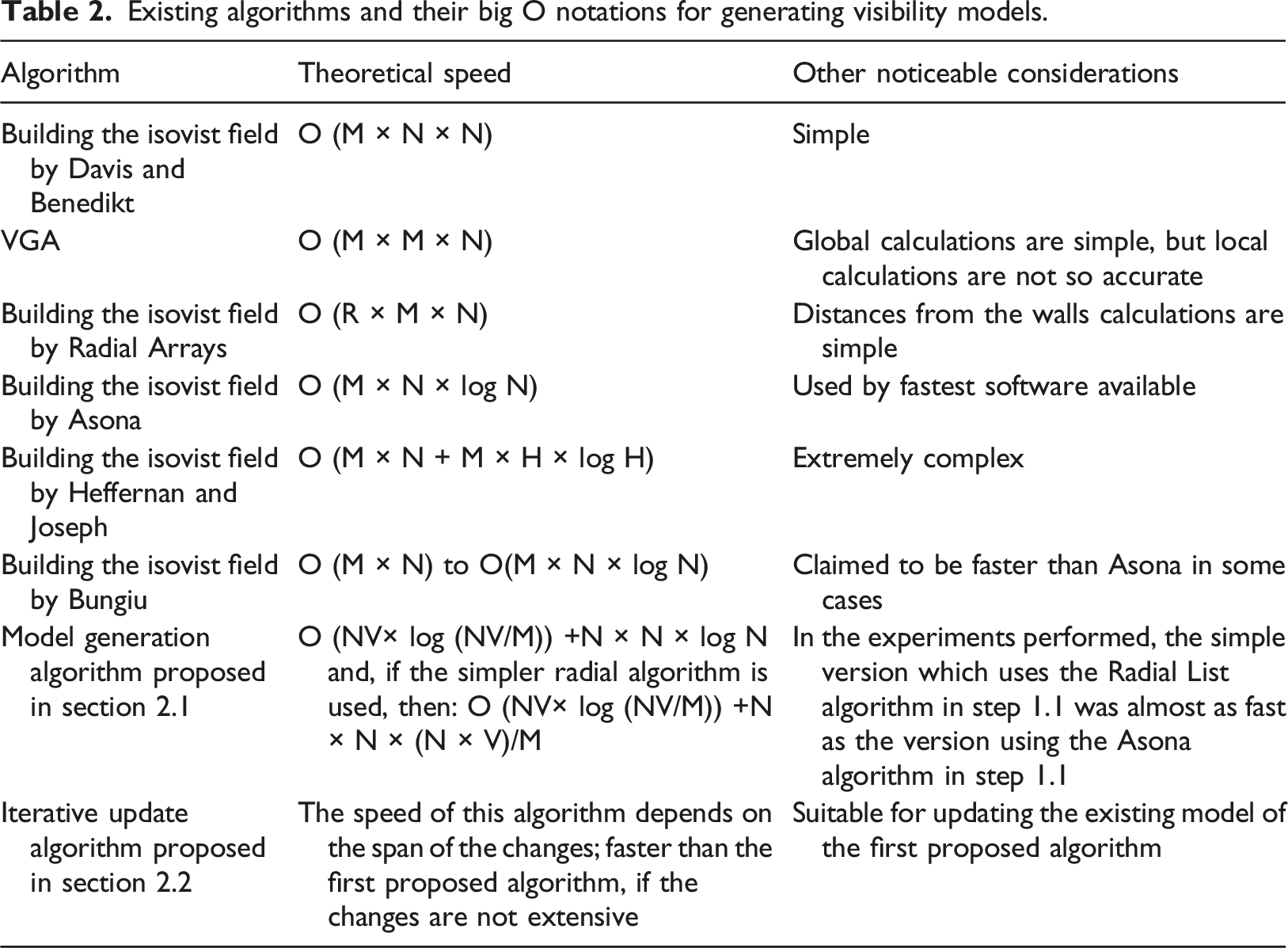
Speed of the two proposed algorithms in theory

In computer sciences, to calculate the theoretical bounds on the speed (time complexity) of an algorithm, which is a common practice, we usually use O notation (order of the function). For comparing and calculating O notation for different algorithms mentioned in this paper, the number of the sample points in the environment is referred to by M, and the number of the corners of the environment, which is roughly equal to the number of the walls, will be N. Let us also suppose that all average corner points can see V sample points of the environment. Considering these variables, the O notation of the proposed algorithm is nearest to O (NV× log (NV/M)) + N × N × log N. (Supplementary Table S1 of part two of the supplementary materials: O notation for different steps of the proposed algorithm). The O notation for creating the isovist field with the Asano algorithm is M × N × log N. So, theoretically, the proposed algorithm is M × log N/V × log (N × V/M), that is, almost M/V times faster than the Asano algorithm. It is possible to compare the O notation of this algorithm with other existing algorithms for generating visibility models (Table 2).

Table 2.

Existing algorithms and their big O notations for generating visibility models.

Algorithm	Theoretical speed	Other noticeable considerations
Building the isovist field by Davis and Benedikt	O (M × N × N)	Simple
VGA	O (M × M × N)	Global calculations are simple, but local calculations are not so accurate
Building the isovist field by Radial Arrays	O (R × M × N)	Distances from the walls calculations are simple
Building the isovist field by Asona	O (M × N × log N)	Used by fastest software available
Building the isovist field by Heffernan and Joseph	O (M × N + M × H × log H)	Extremely complex
Building the isovist field by Bungiu	O (M × N) to O(M × N × log N)	Claimed to be faster than Asona in some cases
Model generation algorithm proposed in section 2.1	O (NV× log (NV/M)) +N × N × log N and, if the simpler radial algorithm is used, then: O (NV× log (NV/M)) +N × N × (N × V)/M	In the experiments performed, the simple version which uses the Radial List algorithm in step 1.1 was almost as fast as the version using the Asona algorithm in step 1.1
Iterative update algorithm proposed in section 2.2	The speed of this algorithm depends on the span of the changes; faster than the first proposed algorithm, if the changes are not extensive	Suitable for updating the existing model of the first proposed algorithm

Memory usage

The memory usage of the proposed algorithm depends on the number of sample points, the number of the corner points in the environment, and the average number of corner points which a sample can see. Experiments show that in a system with 8 GB of RAM, the use of memory at about 600 kg is a problem. Before reaching this range, the time consumption amounts to more than 40 s which is not acceptable for convenient use. This indicates that it is the computing time, not the memory required, that makes the proposed algorithm unusable in very large environments. But if the proposed algorithm is accelerated by techniques such as using graphics card power for parallel processing, the memory usage will be one of the algorithm’s concerns for very large environments. This problem emerges because the algorithm holds the data of the whole isovist polygons of all sample points.

It is possible to save only the changing visual arrows from one point to the next, instead of keeping all the visual arrows of all sample points. With this technique, the memory consumption of the algorithm can be significantly reduced, but the speed of the update algorithm will be somehow reduced. It is also possible to create a desirable balance between memory consumption and deceleration. A more detailed explanation of this technique is available in section 3 of the supplementary materials (modification of the main algorithm to reduce the memory usage).

Speed and accuracy of the new method of calculating distance from the walls

As mentioned before, the fastest way to calculate the distance from the walls with rays is to do it within a generated isovist. Table 3 shows the results of experiments performed to measure the consumption time of this process with different degrees of accuracy.

Table 3.

Test results: Speed of calculating distance from the walls within the isovist with rays for 53,000 sample points.

The angular distance between rays in degrees	3	1	0.5	0
Percentage of slices that are smaller than the distance between the rays	37	20	6	0
Time consumed to calculate (in seconds)	3.6 s	10.2 s	19.9 s	$\infty$
Time consumed to calculate in seconds with the new method	0.8 s	0.8 s	0.8 s	0.8 s

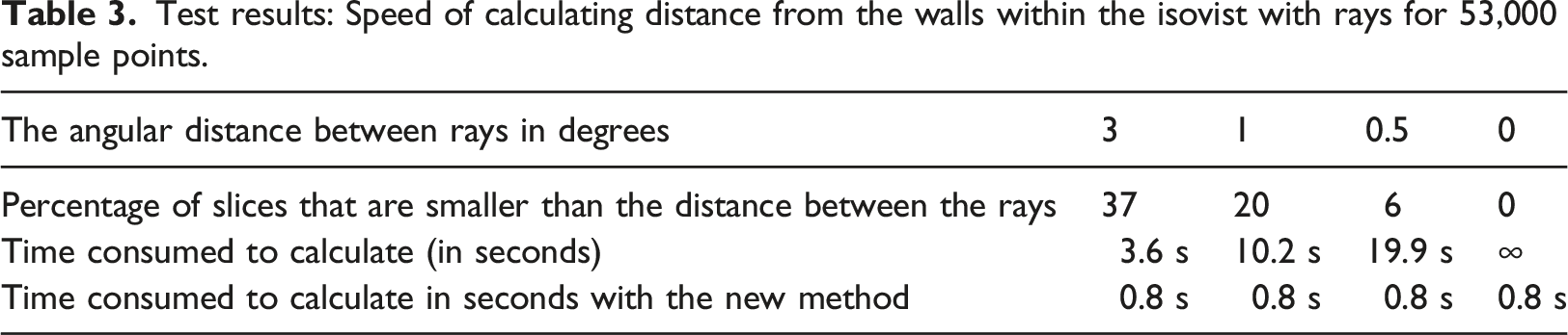
As Table 1 shows, the calculation of the isovist for 53,000 sample points with the first proposed algorithm takes about 7 s. Furthermore, as Table 3 shows, it takes about 10 s to calculate the distance from the walls with one degree of accuracy, which may cause the loss of up to 20% of the slices. Fortunately, with the new method, it takes only 0.8 s to calculate the minimum, maximum, average, variance, skewness, and kurtosis distance from the walls for all 53,000 sample points, and the results will be quite accurate.

Discussion

In this paper, a new algorithm for creating isovist fields was proposed. A secondary algorithm was also proposed to update the model and measurements in case of small changes in the environment. The first proposed algorithm is simple enough to be used by researchers and is much faster than conventional algorithms. The secondary algorithm is even faster when small area changes occur in the environment. Also, a new method for calculating statistical measurements of wall distances in the isovist polygons was proposed which is faster and more accurate than previous methods.

The new algorithm was used in the software development available at https://isovistdesign.com/. The software is open source and is especially useful for defining new measurements for isovist polygons. This software allows the user to calculate a set of selected measurements simultaneously. It also provides a simple platform for algorithmic designing of the environment. We hope that the new algorithm and software will accelerate the development of Visual and Access-based model theory.

Significant research has been done with the aim of better defining the relationship between models with human perception and behavior and defining more meaningful measurements. However, it is not an easy job to find and define new meaningful measurements and provide evidence to support the claim that measurements are correlated with human perception and behavior. The proposed algorithm and the mentioned software provide researchers with a complete form of isovist polygons that can be used in proposing new measurements based on the shape of the polygon. Further, if these proposed measurements are used in the algorithmic design of environments with the provided software, it can be a powerful validation tool for measuring the significance of the proposed measurements. Creating virtual environments with the algorithmic design based on measurements can also serve as a way to prove the causality of the effect of measurements on human perception and feeling.

Besides, it is possible that in translating environmental characteristics to mathematical structures of visibility models, lots of potentially important information will be lost because of the simplification used in the model generation. So, some researchers have tried to improve Visual and Access-based models by extending and improving the information storage structures in the model. For example, Arabacioglu (2010) proposed the use of fuzzy logic in storing semi-transparent objects data, and recently, Ham and Lee (2018) expanded this idea in a specific visual graph of the environment. Some also attempted to define and generate three-dimensional isovist, such as Lu et al. (2019) and KIM et al. (2019). The common problem with such approaches is that the speed of generating their models is far slower than the aforementioned ones, and this makes such models impractical. It should be noted that the main idea of the proposed algorithm in this paper, that is, calculating the visual arrows between the corner points and the sample points at the corner points before calculating the isovist in the sample points, could be used to increase the speed of generating these models considerably and make them more practical.

By improving the visibility models and also better linking the model measurements to human perception and behavior, the visibility models can finally bestow architects great design tool.

Supplemental Material

Supplemental Material - New algorithms for generating isovist field and isovist measurements

Supplemental Material for New algorithms for generating isovist fields and isovist measurements by Arash H Alamdari, Khosro Daneshjoo, and Mansour Yeganeh in Environment and Planning B: Urban Analytics and City Science

Footnotes

Acknowledgment

We thank faculty members of Tarbiat Modares University for their support of this research. We specially thank Dr. Mojtaba Ansari and Dr. Afsane Zarkesh who provided insight and expertise that greatly assisted the research, although they may not agree with all of the interpretations and conclusions of this paper.

Declaration of conflicting interests

The author(s) declared no potential conflicts of interest with respect to the research, authorship, and/or publication of this article.

Funding

The author(s) received no financial support for the research, authorship, and/or publication of this article.

ORCID iDs

Arash Hosseini Alamdari

Mansour Yeganeh

Supplemental Material

Supplemental material for this article is available online.

References

Appleton

(1996) The Experience of Landscape. Chichester: Wiley.

Arabacioglu

(2010) Using fuzzy inference system for architectural space analysis. Applied Soft Computing 10(3): 926–937. DOI: 10.1016/j.asoc.2009.10.011.

Asano

(1985) An efficient algorithm for finding the visibility polygon for a polygonal region with holes. IEICE TRANSACTIONS (1976-1990) 68(9). The Institute of Electronics, Information and Communication Engineers: 557–559.

Batty

(2001) Exploring isovist fields: Space and shape in architectural and urban morphology. Environment and Planning B: Planning and Design 28(1): 123–150. DOI: 10.1068/b2725.

Benedikt

(1979). To take hold of space: isovists and isovist fields. Environment and Planning B: Planning and Design, 6(1): 47–65. London, England: SAGE Publications Sage UK.

Bungiu

Hemmer

Hershberger

, et al. (2014) Efficient computation of visibility polygons. arXiv preprint arXiv:1403.3905.

Foley

Van

Van Dam

, et al. (1996) Computer Graphics: Principles and Practice. Boston, MA: Addison-Wesley Professional.

Ham

Lee

(2018). Space-connector model for representing the geometric properties of connections between spaces. Architectural Science Review 61(6): 429–442. Taylor & Francis,

Heffernan

Mitchell

JSB

(1995) An optimal algorithm for computing visibility in the plane. SIAM Journal on Computing 24(1): 184–201.SIAM.

10.

Hildebrand

(1999) Origins of Architectural Pleasure. Berkeley, CA: Univ of California Press.

11.

KIM

(2019) A new 3D space syntax metric based on 3D isovist capture in urban space using remote sensing technology. Computers, Environment and Urban Systems 74: 74–87. Elsevier. DOI: 10.1016/j.compenvurbsys.2018.11.009.

12.

Gou

, et al. (2019) Three-dimensional visibility graph analysis and its application. Environment and Planning B: Urban Analytics and City Science 46(5): 948–962. SAGE Publications Ltd. DOI: 10.1177/2399808317739893.

13.

McElhinney

(2020) The isovist_App: a basic user guide. Isovist. Available at: https://isovists.org/download/5186/isovist_UserGuide_1-6.pdf.

14.

Ostwald

Dawes

(2020) isovists: Spatio-visual mathematics in architecture. In: Handbook of the Mathematics of the Arts and Sciences (pp. 1–13). Heidelberg, Germany: Springer. DOI: 10.1007/978-3-319-70658-0_5-3.–

15.

Psarra

McElhinney

(2014) Just around the corner from where you are: Probabilistic isovist fields, inference and embodied projection. Journal of Space Syntax 5(1): 109–132.

16.

Polygon Filling Algorithm-Tutorialspoint (n.d.). Available at https://www.tutorialspoint.com/computer_graphics/polygon_filling_algorithm.htm (accessed 11 October 2020.

17.

Schneider

Koenig

(2012) Exploring the generative potential of isovist fields-the evolutionary generation of urban layouts based on isovist field properties.In: 30th International Conference on Education and research in Computer Aided Architectural Design in Europe, Prag, Czech Republic, 15 Sep 2012.

18.

Turner

(2001) A program to perform visibility graph analysis. Proceedings. 3rd International Space Syntax Symposium Atlanta 2001, Atlanta, USA, 2001. academia.edu. https://www.academia.edu/download/3241268/turner01depthmap.pdf

19.

Wineman J Turner J Psarra S , et al. (2007) Syntax2D: An open source software platform for space syntax analysis. In: Proceedings 6th International Space Syntax Symposium, Istanbul, Turkey, 12-15 June 2007. pp. 23–26. http://darts.uncc.edu/sites/darts.uncc.edu/files/papers/Syntax-2D.pdf (accessed 26 May 2020.

Supplementary Material

Please find the following supplemental material available below.

For Open Access articles published under a Creative Commons License, all supplemental material carries the same license as the article it is associated with.

For non-Open Access articles published, all supplemental material carries a non-exclusive license, and permission requests for re-use of supplemental material or any part of supplemental material shall be sent directly to the copyright owner as specified in the copyright notice associated with the article.

0.00 MB

0.38 MB