Exploring temporal variability in travel patterns on public transit using big smart card data

Abstract

Passengers generate travel behaviours on public transit, whose variations deserve an exploration with an aim to guide daily-updated managements. In this study, we investigate temporal variability in travel patterns for over 3.3 million passengers across 120 days who use public transit in Beijing. Temporal variability is characterized by a series of features in terms of space coverage, travel distance and travel frequency, based on which, passengers are clustered into two types, that is, commuters with daily travel routines, and non-commuters who do not. How, and to which extent, they change travel patterns over time are examined, with using approaches concerning multivariate regression and curve fitting. Results show that, (1) commuters are more likely to travel longer but cover less territory than non-commuters on weekdays, while the opposite patterns occur on weekends. The variation of day of week affects commuters less, compared to non-commuters, due to more fixed schedules, as expected; (2) travel distance and frequency are found to increase faster, more linearly, than space-coverage features, the last of which experience a progressive decreasing of marginal increases before reaching a plateau. The above findings facilitate transport practitioners to design sound management schemes for passengers in different categories.

Keywords

Public transit travel patterns temporal variability smart card data

Introduction

Passengers generate a massive amount of trips when taking public transportation facilities over time. These trips are documented as digital records by smart cards in a sound resolution and a mega sample size. Each record possesses tap-on and tap-off points with timestamps en route, thus constituting a solid database to uncover invisible patterns in passengers’ travel behaviours. The hidden patterns are named as travel patterns, a well-known term used by many smart-data-related studies (Dharmowijoyo et al., 2016; Shan et al., 2017; Medina and Arturo, 2018; Yong et al., 2018; Zhang et al., 2018).

Mining passengers’ travel patterns receive much attention (Gonzalez et al., 2008; Kitamura et al., 2009; Ma et al., 2013; Susilo and Axhausen, 2014). Commuters, are a typical type of passengers preferred by this topic, who possess strong repetitions when travelling between fixed places in fixed time (Huang et al., 2019; Kieu et al., 2015; Ma et al., 2017). Non-commuters, instead, exhibit more variability in space or/and time by transit for non-obligatory activities such as grocery shopping or recreation (Dharmowijoyo et al., 2016; Misra and Bhat, 2000), making them hard to be detected by regularity-based approaches. In this regard, variability analysis is crucial, which brings a complementary view in elaborating travel patterns (Zhong et al., 2015). Besides, variability always exists in passengers’ travel behaviours, no matter what category they belong to, since passengers are kept influenced by changing factors (Kandt and Leak, 2019) such as social factors (e.g. personal needs, preferences), demographic factors (e.g. ages, genders) or temporal factors (e.g. day of week, month of year). Revealing how, and to which extent, variability develops over time may help guide daily-updated management schemes or sound land-use design in a long run.

Travel patterns have been characterized by a series of features such as activity space (Schonfelder and Axhausen, 2003; Fan and Khattak, 2008; Kitamura et al., 2009), travel distance (Gonzalez et al., 2008; Zhou and Long, 2014), travel time (Yildirimoglu et al., 2015) or travel frequency (Hasanzadeh et al., 2019). Based on the above characterization, variability can be represented in two types, namely, day-to-day variability and day-accumulated variability. The first type, which has been investigated by most studies, such as Jarv et al. (2014), Raux et al. (2016), Dharmowijoyo et al. (2018), measures increment values of a feature between every two consecutive days, to describe variability in travel patterns day by day. The second type measures the accumulated or maximum values of a feature by each day, to uncover to which extent variability develops over time. Currently, few studies shed light on the latter one, making it hard to grasp to which extent variability develops when time grows.

To better understand this issue, this study aims to examine variability in terms of day-to-day variation and day-accumulated variation, to uncover how, and to which extent, passengers change their travel patterns over time. Unlike previous studies which worked either on small-scale datasets, or over a short period of time, this analysis is based on a big smart card dataset on Beijing public transit generated by over 3 million passengers across 120 days. Individual travel pattern is firstly characterized by six features, whose temporal series are built to portray temporal variability. Based on the feature series, passengers are segmented into different groups. Variation analysis is conducted on the feature series to examine the differences of temporal variability in travel patterns for passengers in the derived categories, before investigating how, and to which extent, these variations distribute globally and locally over time.

Overall, our contributions are summarized as follows:

1. We explore how, and to which extent, passengers in different categories vary travel patterns on both day-to-day and day-accumulated bases. Local and global variation trends are both explored, with an aim to give a comprehensive analysis of temporal variability with multiple perspectives.

2. We compare the differences of temporal variability in travel patterns for different groups of passengers by using a big dataset across multiple days, with an aim to provide sound management schemes for different types of passengers when they compete for public transit resources.

For the remainder of this paper, related work is summarized in the Related Work section, with data and methods introduced in the Data Collection section and the Methodology section. Results are elaborated in the Results section, followed by discussions and conclusions given in Section 6.

Related Work

The way to characterize travel patterns is firstly reviewed, followed by a summary of how to measure temporal variability in travel patterns.

Characterize travel patterns

Passengers’ travel patterns have been quantified by a lot of features such as activity space (Schonfelder and Axhausen, 2003; Fan and Khattak, 2008; Kitamura et al., 2009), travel distance (Gonzalez et al., 2008; Zhou and Long, 2014), travel time (Yildirimoglu et al., 2015) or travel frequency (Hasanzadeh et al., 2019). Take Gonzalez’s study (2008), for example, the research collected a week’s trajectories of 40 mobile phone users, and extracted travel distance to measure users’ travel patterns in a global view. Zhou and Long (2014) chose two distance-related indices to explore the distribution of job-housing commuting in Beijing. Yildirimoglu et al. (2015) selected travel time, while Hasanzadeh et al. (2019) chose trip frequency, to describe human travel patterns. These non-geometric features can be used to portray travel patterns in this paper. As to geometric features, Schonfelder and Axhausen (2003) adopted a confidence ellipse to model an activity space, and quantified it with several inherent features, such as area, perimeter or vertical distance, for a further calculation. Unlike an ellipse with regular shapes, a convex hull was employed by Fan and Khattak (2008) to create a more arbitrary geometric diagram, by drawing minimum boundaries around candidate locations. It was testified to obtain a higher proximity and a less bias than an ellipse in mapping geometric space coverage with random diagrams (Lee et al., 2016). Instead of using a two-dimensional ellipse or convex hull, Kitamura et al. (2009) built a three-dimensional space–time prism, which is constrained by multiple parameters, such as fixed anchor points or maximum travel velocity, to model space coverage of passengers based on their morning trips. Though possessing an extra dimension of time, a prism is reluctant to describe raw travel trajectories, not only due to its uncertainty in measuring relevant constrains (Leung et al., 2016), but also due to its higher computational complexity than convex-hull-based approaches in dealing with big data. In this regard, a convex hull is more widely used to describe geometric space coverage of passengers due to its arbitrariness and low dimensionality. Overall, the above features form a solid basis to characterize travel patterns, although they were not elaborated into fine temporal units for temporal variability discovery.

Measure temporal variability in travel patterns

To explore temporal variability, previous studies sliced a timeline into finer units, such as a day, a week, a month or a year, based on which, time series of features were extracted. For example, Jarv et al. (2014) sampled the call detail records of 1310 mobile phone users across 12 months, to capture their monthly variability in travel patterns. The research found a modest monthly variation in the number of travel locations, as well as a great variation in space coverage. Chu (2015) sampled the smart card data of 330,140 travellers across two years to examine variability in travel patterns. The research found that mobility indicators, including the number of active cards and trip rate, presented a greater variation than activity location daily, weekly and yearly. Raux et al. (2016) cut a timeline into a daily unit, and extracted daily-based trip counts for 707 individuals over seven days by using a sequence alignment method (SAM). The research confirmed a marginal day-to-day variability in the parameter. Day-to-day variability was also investigated by Dharmowijoyo et al. (2018), who extracted the diaries of 732 individuals across 21 days. The research analyzed the interaction coefficients between personal travel activities and demographic attributes like age or gender, and found that the socio-demographics characteristics significantly influenced individual travel frequency or distance every day. Overall, most of the above studies cut timelines into daily units to analyze day-to-day variability in travel patterns, without shedding light on day-accumulated variability, thus making it hard to understand to which extent variability develops over time. This is one research focus in this paper.

Previous studies also found that variability differed in weekdays versus weekends (Zhong et al., 2015), in workers versus non-workers (Dharmowijoyo et al., 2016; Briand et al., 2017; Huang et al., 2018; Yuan and Raubal, 2016) and in intrapersonal versus interpersonal levels (Zhang et al., 2018), with the ever-increasing of time. For example, Zhong et al. (2015) collected one-week smart card data to investigate the differences of temporal variability in trip frequency among different passengers. The research demonstrated that trip frequency not only varied from weekdays to weekends, from person to person, but also from place to place. Yuan and Raubal (2016) sampled 100 subjects for commuters and non-commuters, and characterized their travel patterns by three predefined metrics, that is, spatial index, radium and entropy. The research fitted each parameter with a Weibull distribution, and found that distinct distribution patterns existed among different groups of subjects. Yet, how travel behaviours varied over time was not explored, which is indeed our main focus. Dharmowijoyo et al. (2016) also targeted at these two types of passengers, and examined their day-to-day variability in three features, that is, travel time, travel frequency and travel distance. The results showed that different groups of individuals exhibited distinct trade-off mechanisms. Daily commuting shaped commuters’ travel time regularly leading to a more stable variability in it than non-commuters. Briand et al. (2017) sampled five-year smart data containing 82,223 cards to investigate the differences of year-to-year variability in temporal activities among different passengers. The longitudinal analysis demonstrated a relative stability of public transport usage. Similar as Briand et al. (2017), Huang et al. (2018) conducted a longitudinal study to examine year-to-year variability in travelling time by using a sampled seven-year dataset that contained 4248 commuters. The study found that commuters characterized with different mobility groups presented distinct job-housing dynamics over years. Zhang et al. (2018) synthesized one-week travel behaviours from a single-day household travel survey and extracted trip frequency, travel time and travel location for 317 subjects, whose daily variability was investigated in intrapersonal versus interpersonal levels. The research found that the distribution of interpersonal variability in a single day was similar to that of intrapersonal variability in multiple days. Overall, the above findings were derived either based on small-scale datasets, or over a short period of time. Given a large-scale dataset across multiple days, whether such variability differences remain still needs a further discussion. This is another research focus in this paper.

To sum up, previous studies measured day-to-day variability to explore how passengers alter their travel patterns day by day, companied with a neglect of exploring to which extent such variability develops with the accumulation of days. To address this issue, we examine variability on both day-to-day and day-accumulated bases, so as to give a comprehensive analysis of temporal variability with multiple perspectives. Meanwhile, unlike previous studies which worked on small-scale datasets or over short periods of time, we adopt a large-scale dataset across multiple days, to get a bigger picture of temporal variation differences in travel patterns for different groups of people. Statistical analysis and model fitting are adopted to uncover how, and to which extent, travel patterns vary over time.

Data Collection

To measure temporal variability in travel patterns, the data source used in this paper is the big transaction records collected by automated fare collection (AFC) systems in Beijing in 2015, when passengers swiped their smart cards to board or alight. At the time, Beijing public transit network maintained and operated 41,970 bus stops and 325 subway stations, which were connected by 763 bus routes and 16 subway lines, respectively. The dataset includes 120 days of records in July, August, September and November. Holidays are excluded from our dataset, since scarce and distinct travel patterns, for example, travelling out of the city, may emerge. Invalid transaction records are filtered out, leaving 769,413,168 valid records.

The above valid records may be correlated to one another, if a passenger ‘firstly travels by bus and then by subway’. With owning short time gaps and close spatial distances, correlated records generated by one individual can build a new trip chain, whose construction way is specifically introduced in previous work (Kieu et al., 2015; Ma et al., 2013; Zhao et al., 2019). Travellers who generate at least one trip chain by transit in five different days are selected, so that infrequent transit riders are excluded. In total, 741,163,566 trip chains formed by 3,922,131 cards are derived, with each chain containing fields like smart card IDs, entry/exit station IDs, station coordinates and the corresponding timestamps.

Methodology

Four steps are included in this section to explore temporal variability in travel patterns. Firstly, individual travel pattern is characterized by six features concerning space coverage, travel distance and travel frequency. Each feature generates a temporal series to portray its temporal variability, all of which are then clustered by the k-means++ algorithm to derive passengers’ categories. After validating the clustering results with priori rules, variation analysis is conducted on these feature series via multivariate ordinary least square (MOLS) regression, to examine the differences of temporal variability in travel patterns for different groups of passengers. Finally, the probability distribution functions (PDFs) of all the feature series are further fitted by priori probabilistic models, to investigate how, and to which extent these variations distribute over time. The overall framework of this paper is shown in Figure 1.

Figure 1.

The overall framework of this study.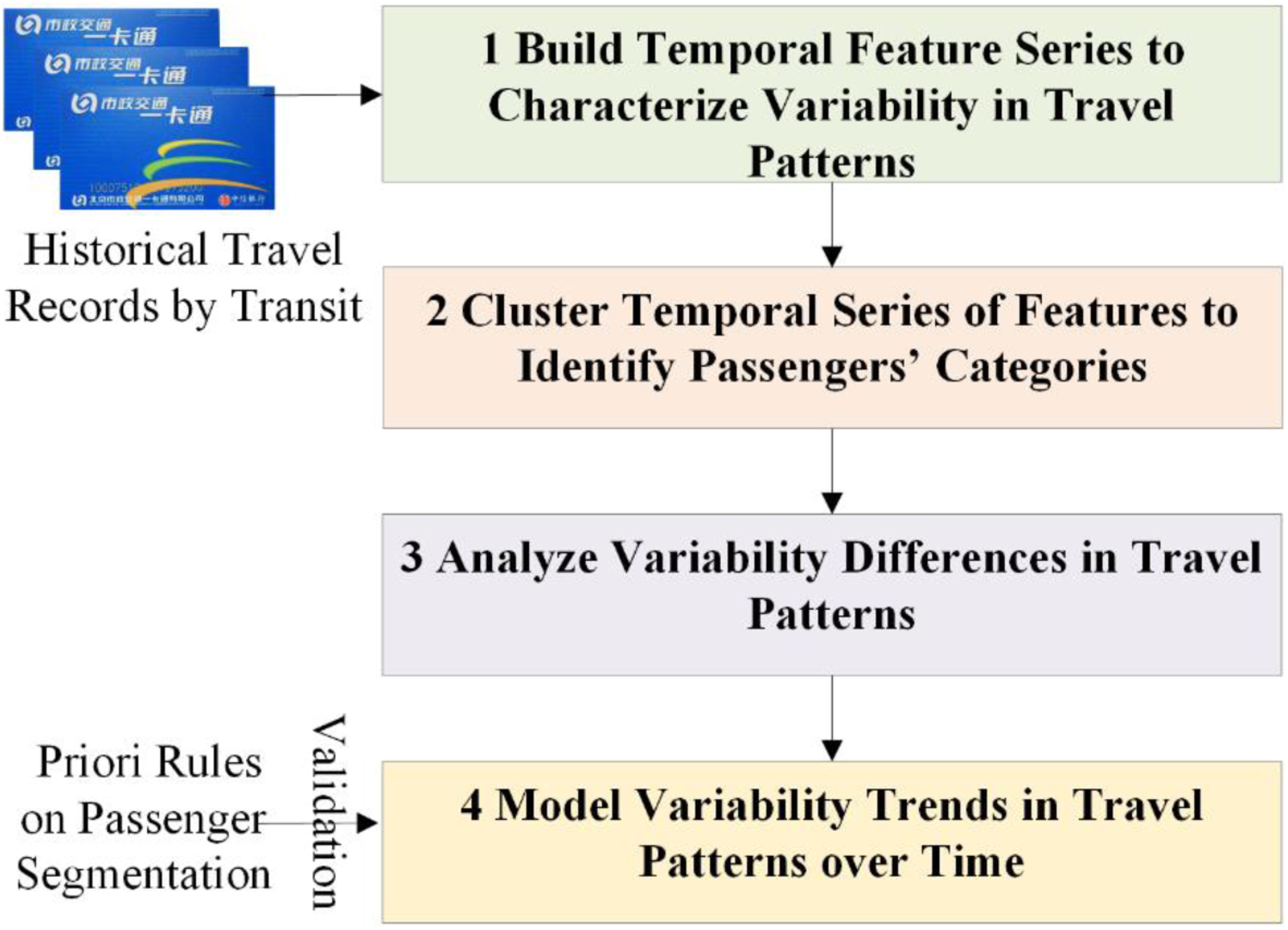

Build temporal series of features to characterize variability in travel patterns

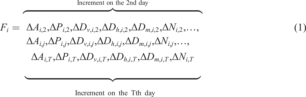
Based on the aforementioned work summarized in the Characterize Travel Patterns section, passengers’ travel patterns are characterized by six features in this paper, namely, travel distance, travel frequency and another four geometrical features concerning space coverage. Travel distance refers to the overall trip distances per day and is quantified by the Manhattan distance ( $D_{m}$ ). Travel frequency indicates the overall number of trips ( $N$ ) per day. Space coverage is shaped by a convex hull drawn along the boundaries of a daily-expanded location set ( $Ω$ ) containing all stations visited. For calculation convenience, it is further instantiated by four inherent geometrical features, namely, area ( $A$ ), perimeter ( $P$ ) and the maximum distances in vertical¹ ( $D_{v}$ ) or horizontal ( $D_{h}$ ) directions.

Denote f as any of the features mentioned above. $f \in {D_{m}, N, A, P, D_{v}, D_{h}}$ . It is represented in two forms. In the first form, f is quantified by its value differences ( $Δ f$ ) between every two consecutive days, to render day-to-day variations, for example, abrupt changes. In the second form, f is quantified by its accumulated values ( $\sum f$ ) by every single day, to quantify day-accumulated variability, for example, variation extents. For individual i, his/her day-to-day variability and day-accumulated variability of feature f on day j are particularly instantiated as $Δ f_{i} = (Δ f_{i, 2}, \dots, Δ f_{i, j}, \dots, Δ f_{i, T}}$ , and $\sum f_{i} = (f_{i, \sum 2}, \dots, f_{i, \sum j}, \dots, f_{i, \sum T})$ , respectively. $Δ f_{i, j}$ is the value difference of feature f on days j and j−1 and $Δ f_{i, j} = f_{i, \sum j} - f_{i, \sum j - 1}$ . $f_{i, \sum j}$ and $f_{i, \sum j - 1}$ are the accumulated values of feature f, with reaching a summit by day j or j−1, respectively. $2 \leq j \leq T$ . $T$ is the overall 120 days adopted in this paper.

Cluster temporal series of features to identify passengers’ categories

The above feature series are re-organized for clustering to derive passengers’ categories, which are further validated by priori rules and knowledge.

Cluster temporal series of features

With no prior knowledge of passengers’ group labels, an unsupervised algorithm named the k-Means++ (Arthur and Vassilvitskii, 2007) is conducted on the derived feature matrix F to cluster passengers. The algorithm is a simple and fast algorithm that firstly seeds initial centres and then clusters data into k groups. It is chosen for its superiority in dealing with big data. Passengers holding similar day-to-day variation trends in feature series are automatically clustered into one group.

The input of the algorithm is the derived feature matrix F=[ $F_{i}$ ], where $F_{i}$ of individual i is the feature series that combines the above six feature series together. $F_{i}$ is shown in equation (1), to describe day-to-day variability in travel patterns.

F_{i} = \overset{Increment on the 2 nd day}{\overset{⏟}{\begin{array}{l} Δ A_{i, 2}, Δ P_{i, 2}, Δ D_{v, i, 2}, Δ D_{h, i, 2}, Δ D_{m, i, 2}, Δ N_{i, 2}, \dots, \\ Δ A_{i, j}, Δ P_{i, j}, Δ D_{v, i, j}, Δ D_{h, i, j}, Δ D_{m, i, j}, Δ N_{i, j}, \dots, \\ Δ A_{i, T}, Δ P_{i, T}, Δ D_{v, i, T}, Δ D_{h, i, T}, Δ D_{m, i, T}, Δ N_{i, T} \\ ⏟ \\ Increment on the Tth day \end{array}}}

(1)

Two metrics named SSE and SSB are employed to evaluate clustering performances (Kumar et al., 2018; Han et al., 2012; Zhao et al., 2019). The former one measures the total squared distance distortion within clusters, while the latter one records the total squared distance distortion between clusters. The algorithm converges when SSE and SSB reach their minimum and maximum values, respectively. At the time, the degree of cohesion in each cluster becomes the highest. So does the degree of separation between clusters. These two metrics are represented by equations (2) and (3), respectively, where $c_{k}$ is the cluster centre for the $k_{t h}$ cluster. c is the cluster centre of the dataset. $m_{k}$ is the number of passengers in the $k_{t h}$ cluster.

S S E = \sum_{k = 1}^{K} \sum_{x_{i} \in c_{k}} d i s t {(x_{i}, c_{k})}^{2}

(2)

S S B = \sum_{k = 1}^{K} m_{k} d i s t {(c, c_{k})}^{2}

(3)

Validate clustering performances

The above clustering performances are validated by an empirical approach obtained from priori rules and knowledge (Huang et al., 2019; Ma et al., 2017; Wen et al., 2016; Zhao et al., 2020; Zhou and Long, 2014). It roughly divides passengers into two groups, that is, commuters and non-commuters, based on the following procedures.

1. For each passenger, visited stations, at which the activity duration time between two consecutive trip chains, determined by the arrival time of the former trip chain and the departure time of the next trip chain, is longer than six hours, are labelled as a set of hotspots. This temporal benchmark is set based on the statistical annual report on average working hours in Beijing (Huang et al., 2019).

2. The visited station that has the highest frequency in the set built by Rule (1) is labelled as home (Zhou and Long, 2014).

3. The station which has the second highest frequency in the set and is visited more than three days a week, is stamped as the routine place (Zhou and Long, 2014). The corresponding week is denoted as a routine week in this paper. An implicit assumption given here is that an individual who maintains a regular social activity conducts routine trips to the same station at least three days a week.

4. When the routine weeks identified by Rule (3) exceed five weeks, the 95th percentile ratio of routine weeks among all smart card holders, we classify the passenger as a commuter.

The derived segmentation results of passenger categories become the ground truth data in this paper. F1 score, a harmonic mean of precision and recall (Han et al., 2012), is calculated to evaluate the clustering performances. The higher the score is, the better the clustering performances are. F1 score is denoted by equation (4), where TP, FP and FN refer to the number of true positives,² false positives and false negatives, respectively.

{\begin{matrix} F 1 = \frac{2 \times p r e c i s i o n \times r e c a l l}{p r e c i s o n + r e c a l l} \\ p r e c i s i o n = \frac{T P}{T P + F P} \\ r e c a l l = \frac{T P}{T P + F N} \end{matrix}

(4)

Analyze variability differences in travel patterns

Measure to which extent variability develops over time

A group of experiments on variation analysis are conducted to measure to which extent variability develops over time for different groups of passengers, whose variability differences in travel patterns are further compared, with results presented in the Measure to Which Extent Variability Develops Over Time section.

Particularly, multivariate ordinary least square (MOLS) regression is adopted, with a typical model denoted in equation (5) at 0.001 significance level. Each feature $Δ f_{c, i, j}$ , which is measured on day j for individual i who belongs to category c, is treated as a dependent variable. ‘c’ has two options, that is, ‘commuter’ or ‘non-commuter’. The temporal elements $D a y_{t d}$ and $M o n t h_{t m}$ are both treated as independent variables. $D a y_{t d}$ relates to days, with ‘td’ ranging from 1 (Monday) to 6 (Saturday). $t d \neq 7$ , since Sunday serves as the reference group of days. $M o n t h_{t m}$ relates to months. ‘ $t m$ ’ owns three options, that is, 7, 8 and 9, with referring to July, August and September, respectively. $t d \neq 11$ , since November is the reference group of months. $α_{c, t d}$ and $β_{c, t m}$ are two coefficient estimates of day-of-week and month-of-year variables, respectively. They are measured to indicate to which extent an independent variable influences a dependent one for either commuters or non-commuters. $C_{c}$ is a constant intercept. Altogether, 2 (commuters and non-commuters) × 6 (features) = 12 groups of experiments are conducted, with variation results elaborated in the Measure to Which Extent Variability Develops Over Time section.

Δ f_{c, i, j} \sim C_{c} + \sum_{t d ϵ [1,6]} α_{c, t d} D a y_{t d} + \sum_{t m ϵ [7,9]} β_{c, t m} M o n t h_{t m}

(5)

Measure how variability distributes over time

How day-to-day variability distributes over time is also measured for different groups of passengers. Particularly, the probability density function (PDF) of each feature series that is extracted in the Build Temporal Series of Features to Characterize Variability in Travel Patterns section is fitted by five probabilistic models, that is, Exponential, Gamma, Levy, Lognormal and Weibull, with an optimum curve chosen to describe its day-to-day variability. Derived curves representing different groups of passengers are further compared to investigate how distinct they are over time. Specific results are elaborated in the Measure How Variability Distributes Over Time section.

Model variability trends in travel patterns over time

Temporal evolution trends in travel patterns are modelled on both day-accumulated and day-to-day bases, to reach two aims: (1) grasping a global variation trend in travel patterns; (2) uncovering how the above trends vary by a local rate. For any feature, its daily mode on either basis is measured and aligned into a temporal mode series. The given 120 research days are organized into a temporal sequence numbered from 1 to 120. Plots are drawn for each mode series to describe its association with time, with an optimum fitting curve chosen from five candidate distribution models, that is, Exponential, Linear, Lognormal, Power and Bivariate polynomial, to better illustrate how, and to which extent, a feature evolves over time. Specific results are presented in the Model Variability Trends in Travel Patterns Over Time section.

Results

Analyze clustering results

Since the k-means++ algorithm requires an initialization of a clustering number, a group of sensitivity experiments are conducted, whose clustering performances are depicted in Figure 2. As cluster number rises from 1 to 6, SSE experiences a decrease, with a concurring increase in SSB. An intersection point emerges around 2 for the first time, which is thus set to be the optimum cluster number of passenger groups in this paper.

Figure 2.

Determination of an optimum cluster number.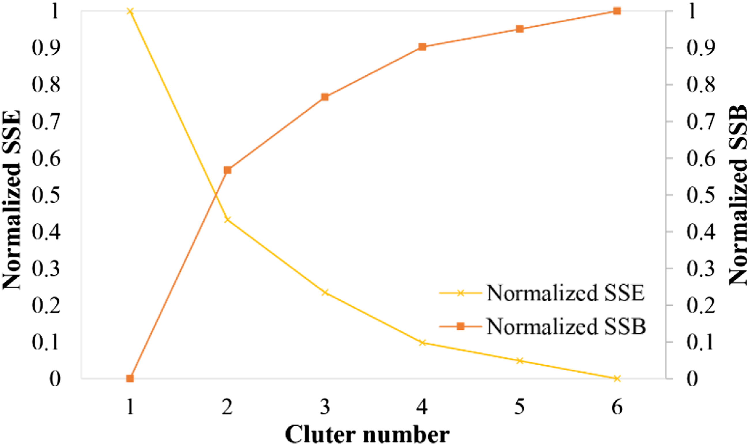

The empirical segmentation results of commuters and non-commuters, as derived in the Validate Clustering Performances section, are employed to supervise the above clustering performances with F1 score, precision and recall measured to be 0.84, 0.85 and 0.84, respectively. These values indicate that 84% passengers sampled from the same dataset are correctly labelled. In particular, 1,547,292 commuters (46.71%) are detected, together with the remaining 1,765,501 non-commuters. This percentage of commuters is in line with the priori figure reported by Beijing Transportation Institute in 2015 (Wen et al., 2016). They are chosen as subjects in this paper for further analyses.

Figure 3 illustrates the distributions of day-to-day variability and day-accumulated variability across 18 sampled Mondays for commuters and non-commuters. In general, commuters possess higher values in either variation form for all features than non-commuters over time indicating that commuters always travel longer, wider and more frequently than non-commuters every day. On average, a commuter generates 2.45 trips lasting for 18.7 km per day, and covers daily increments of 3.56 km² and 0.47 km in area and perimeter, respectively. These increment values are all higher than those of non-commuters. For all passengers, the average daily increment value of vertical distance is slightly higher than the horizontal one. This indicates a larger space coverage in the ‘North-South’ direction, where more developed workplaces can be found such as the Chinese Silicon ZhongGuanCun, the mega biopharmaceutical base XiErQi and the giant residence districts named TianTongYuan and YiZhuang.

Figure 3.

Distributions of day-to-day and day-accumulated variability of commuters and non-commuters.³ (a) Distribution of day-to-day variability for commuters, (b) distribution of day-to-day variability for non-commuters, (c) distribution of day-accumulated variability for commuters and (d) distribution of day-accumulated variability for non-commuters.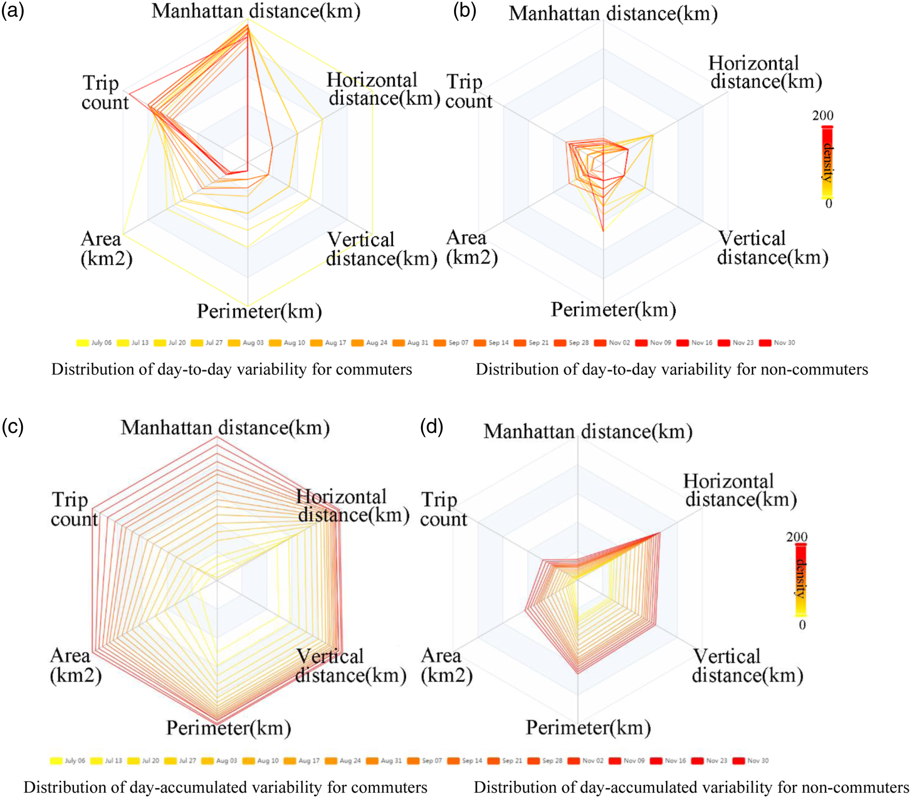

Figure 4 illustrates the distribution of average number of trips of commuters or non-commuters by time of day on weekdays and weekends. Commuters present sharp morning and evening peaks on weekdays for routine affairs (e.g. working or going to school). Meanwhile, two slight peaks are generated by non-commuters, who might head towards government agencies or enterprises in office hours for business, or towards schools to deliver (/pick up) kids in mornings or afternoons. Daily trips are more evenly distributed over a day for the two types of passengers during weekends.

Figure 4.

Average hourly number of trips of commuters and non-commuters.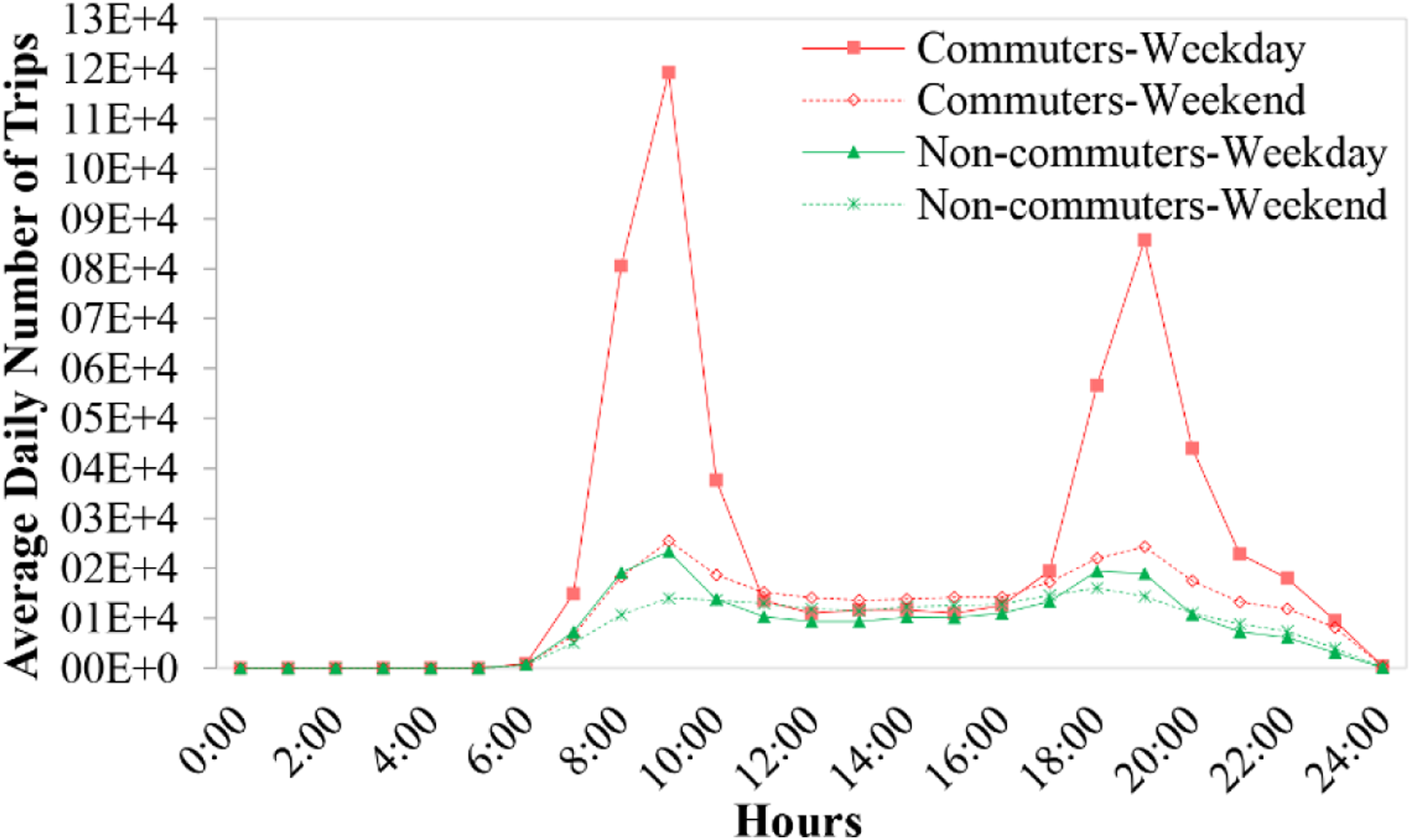

Analyze variability differences in travel patterns

Measure to which extent variability develops over time

The MOLS regression results of the six features on temporal variables are presented in Table 1 to explain how these features vary by day of week or month of year.

Table 1.

Regressions of the features on temporal elements.

Independent variables	Dependent variables
Independent variables	Manhattan distance increment	Trip count increment	Area increment	Perimeter increment	Vertical distance increment	Horizontal distance increment
Commuters
Constant	23.26	2.88	6.35	1.13	0.37	0.35
Monday	0.76	0.01	−0.88	0.03	0.04	0.03
Tuesday	0.91	0.04	−0.77	0.01	0.03	0.01
Wednesday	0.99	0.10	−0.64	0.11	0.05	0.06
Thursday	0.65	0.05	−0.70	0.01	0.03	0.02
Friday	1.05	0.09	1.02	0.27	0.09	0.08
Saturday	−0.22	−0.14	0.64	0.09	0.02	0.01
July	1.92	0.13	4.97	1.05	0.34	0.33
August	0.48	0.07	3.13	0.80	0.26	0.25
September	0.99	0.15	4.67	1.02	0.33	0.32
Adj. R²	0.07	0.08	0.04	0.02	0.01	0.01
Non-commuters
Constant	13.21	1.01	3.26	0.93	0.35	0.33
Monday	−0.74	−0.02	−0.51	−0.12	−0.02	−0.03
Tuesday	−1.02	−0.02	−0.52	−0.26	−0.02	−0.03
Wednesday	−1.20	−0.09	−0.32	−0.31	−0.04	−0.04
Thursday	−0.38	−0.01	−0.23	−0.24	−0.02	−0.06
Friday	−0.69	−0.01	0.07	−0.09	0.54	−0.02
Saturday	0.41	0.04	0.63	0.02	0.02	0.01
July	1.67	−0.17	−4.79	1.77	0.53	0.59
August	−0.53	−0.08	−3.80	−0.89	0.22	−0.46
September	0.94	−0.15	−4.36	1.43	0.59	0.54
Adj. R²	0.07	0.08	0.03	0.02	0.01	0.01

All coefficients are significant at the 0.001 level.

Day-of-week variation

As shown in Table 1, one phenomenon is found among commuters that weekdays have positive effects on the increments of most of the features, except for area, comparing with Sunday. This is expected, as commuters tend to travel more and longer during weekdays. Many of these trips are conducted for commuting purposes, and contain clear origins and destinations, for example, home and workplaces, with less area covered. During weekends, commuters are more likely to visit multiple stops around home, like grocery stores, restaurants or gyms, with travelling shorter but covering more area. The highest coefficient of area increment emerges on Friday, along with a jump of other features simultaneously, which is probably because a diversity of recreational activities or gatherings are held to celebrate the upcoming weekends. The longest travel distance arises on Wednesday, when multiple events, for example, mid-week leisure activities, on-sale events or membership benefits granted by shopping malls, are organized to attract potential long-distance travels.

For non-commuters, positive coefficients appear on weekends, when longer trips are generated more frequently with a wider coverage of area, comparing with weekdays. Besides that, most of the weekdays are found having negative effects on the increments of the features for non-commuters, with all coefficients being minus with reference to Sunday. These phenomena are caused since non-commuters, who possess more flexibility in travel choices, prefer to travel on weekends, when commuters are significantly fewer. Comparatively, on weekdays, they do not have to or want to, sacrifice their comfort to compete with commuters in a crowded and congested transport environment. Yet, Friday is another story, when the coefficients turn positive on the increments of area and vertical distance. This is because, Friday, as explained before, is a transition day between weekdays and the coming weekends, when organizations like enterprises, shopping malls or communities prefer to hold more entertainment activities to attract passengers in any types to join and celebrate.

Monthly variation

Considering monthly changes, Table 1 shows that the coefficients of the increments of Manhattan distance of passengers in either group are positive in July and September with reference to November indicating a relatively longer distance and higher frequency in travelling. Most of the coefficients of these two parameters in August are much lower than those in July or September indicating an opposite variability pattern in travel distance and frequency. Generally, in November, both commuters and non-commuters tend to generate frequent and short trips, probably around home or workplaces for diverse activities. Weather changes, for example, more comfortable temperatures in July and September (16°C ∼ 25°C), compared to relative high temperatures in August (34°C ∼ 40°C) and low in November (−5°C ∼ 1°C), might help to explain this finding, but need to be confirmed in future studies. Similar monthly variation trends can be found in the increments of perimeter, vertical distance and horizontal distance.

Non-commuters experience a shrinkage of area in July, August and September, compared to November. Unlike non-commuters, commuters keep on covering relatively larger area in the first three months for obligatory activities such as commuting. The above findings are consistent with our assumption that month of year shows different effects on variability in travel patterns among passengers in different categories.

Measure how variability distributes over time

The PDFs of each feature are fitted by the five distribution models mentioned in the Measure How Variability Distributes Over Time section, with the one having the best fit (highest R²) depicted in Figure 5. The similarities between each two optimum curves on weekdays and weekends are further measured using two-term Kolmogorov–Smirnov tests, with results exhibited in Table 2, to support the findings involving variation analysis derived in the Measure to Which Extent Variability Develops Over Time section.

Figure 5.

PDF curves of the increments of the features for commuters and non-commuters on weekdays and weekends. (a) Manhattan distance, (b) trip count, (c) area, (d) perimeter, (e) vertical distance and (f) horizontal distance.

Table 2.

Similarities of pairwise fitting curves describing day-to-day variability of the features on weekdays and weekends.

		Commuters				Non-commuters				Commuters				Non-commuters
		Week-day	Sig	Week-end	Sig	Week-day	Sig	Week-end	Sig	Week-day	Sig	Week-end	Sig	Week-day	Sig	Week-end	Sig
		Manhattan distance								Trip count
Commuters	Weekday	1.00		—		—		—		1.00		—		—		—
Commuters	Weekend	0.01	***	1.00		—		—		1.00		1.00		—		—
Non-commuters	Weekday	0.00	***	0.00	***	1.00		—		0.001	***	0.002	***	1.00		—
Non-commuters	Weekend	0.00	***	0.00	***	0.00	***	1.00		0.00	***	0.01	***	1.00		1.00
		Area								Perimeter
Commuters	Weekday	1.00		—		—		—		1.00		—		—		—
Commuters	Weekend	0.02	**	1.00		—		—	—	0.24		1.00		—		—
Non-commuters	Weekday	0.00	***	0.00	***	1.00		—		0.31		0.00	***	1.00		—
Non-commuters	Weekend	0.00	***	0.00	***	0.02	**	1.00		1.00		0.39		0.24		1.00
		Vertical distance								Horizontal distance
Commuters	Weekday	1.00		—		—		—		1.00		—		—		—
Commuters	Weekend	0.98		1.00		—		—		0.99		1.00		—		—
Non-commuters	Weekday	0.22		0.03	**	1.00		—		0.61		0.19		1.00		—
Non-commuters	Weekend	0.90		0.22		0.90		1.00		0.99		0.61		0.99		1.00

∗∗∗p-Value<0.001, ∗∗p-value<0.01. ‘Sig’ is short for significance.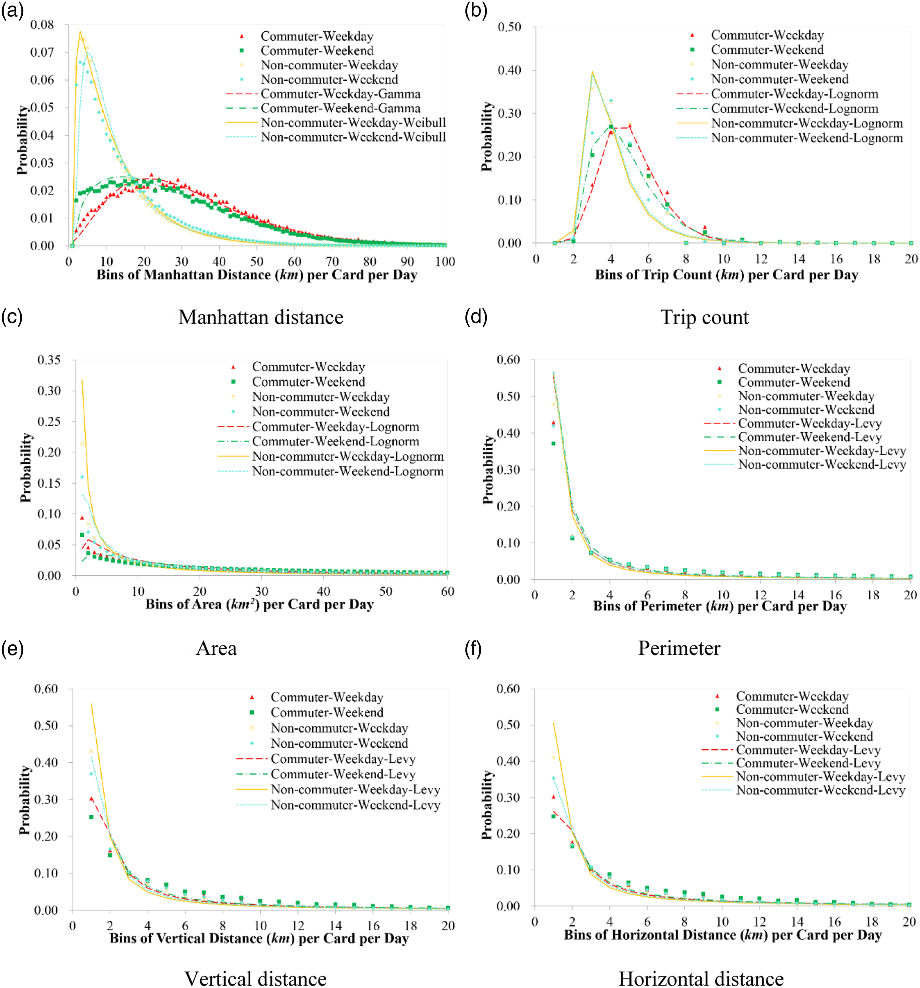

The PDF curves of the increments in Manhattan distance (Figure 5 (a)) and trip count (Figure 5 (b)), present $\cap^{}$ -shape. The mode of the increment in distance lies between 18 km to 24 km with the probability around 0.03 for commuters, considerably higher than that of non-commuters, which is around 3 km to 5 km with the probability around 0.07. This phenomenon corroborates the result given in the Measure to Which Extent Variability Develops Over Time section that commuters generate longer trips on average, compared to non-commuters, in Beijing. As to the increment in trip count, its mode lies around 5 for commuters, higher than the mode of 3 for non-commuters. This finding is in line with the phenomenon shown in Figure 4 that the average hourly number of trips generated by commuters on weekdays is higher than other types. The above two conclusions are supported by the similarity tests on pairwise PDF curves, as shown in Table 2. Focussing on the PDF curves of the increments in Manhattan distance or trip count, commuters show significant differences from non-commuters on either weekdays or weekends.

The PDF curves of the increments in area, as shown in Figure 4 (c), go down sharply because distances induce impedance when travelling between different spots, which is consistent with the gravity model (Fotheringham and O’Kelly, 1989). Lognormal distribution better fits the PDFs of area increment for both types of passengers (Gonzalez et al., 2008).

The PDF curves of the increments in perimeter (Figure 5 (d)), vertical (Figure 5 (e)) and horizontal (Figure 5 (f)) distances, all possess striking declining trends. The PDF distributions of these parameters are explained by Levy distribution. Table 2 also indicates that the PDF curves of perimeter, as well as vertical distance, of commuters on weekends, significantly differ from those of non-commuters on weekdays. Other than these differences, no significant differences are found between any pair of PDF curves in Figure 5 (d) to Figure 5 (f).

Model variability trends in travel patterns over time

For each feature, four plots are drawn in Figure 6 for commuters and non-commuters to model its variability trends over time. The two plots placed in the centre of the figure are designed to examine to which extent a feature evolves with the accumulation of days, while the other two plots placed in the top left corner of the figure indicates how this evolution trend varies on a day-to-day basis.

Figure 6.

Distributions of variability in travel patterns on both day-accumulated and day-to-day bases for commuters and non-commuters. (a) Manhattan distance, (b) trip count, (c) area, (d) perimeter, (e) vertical distance and (f) horizontal distance.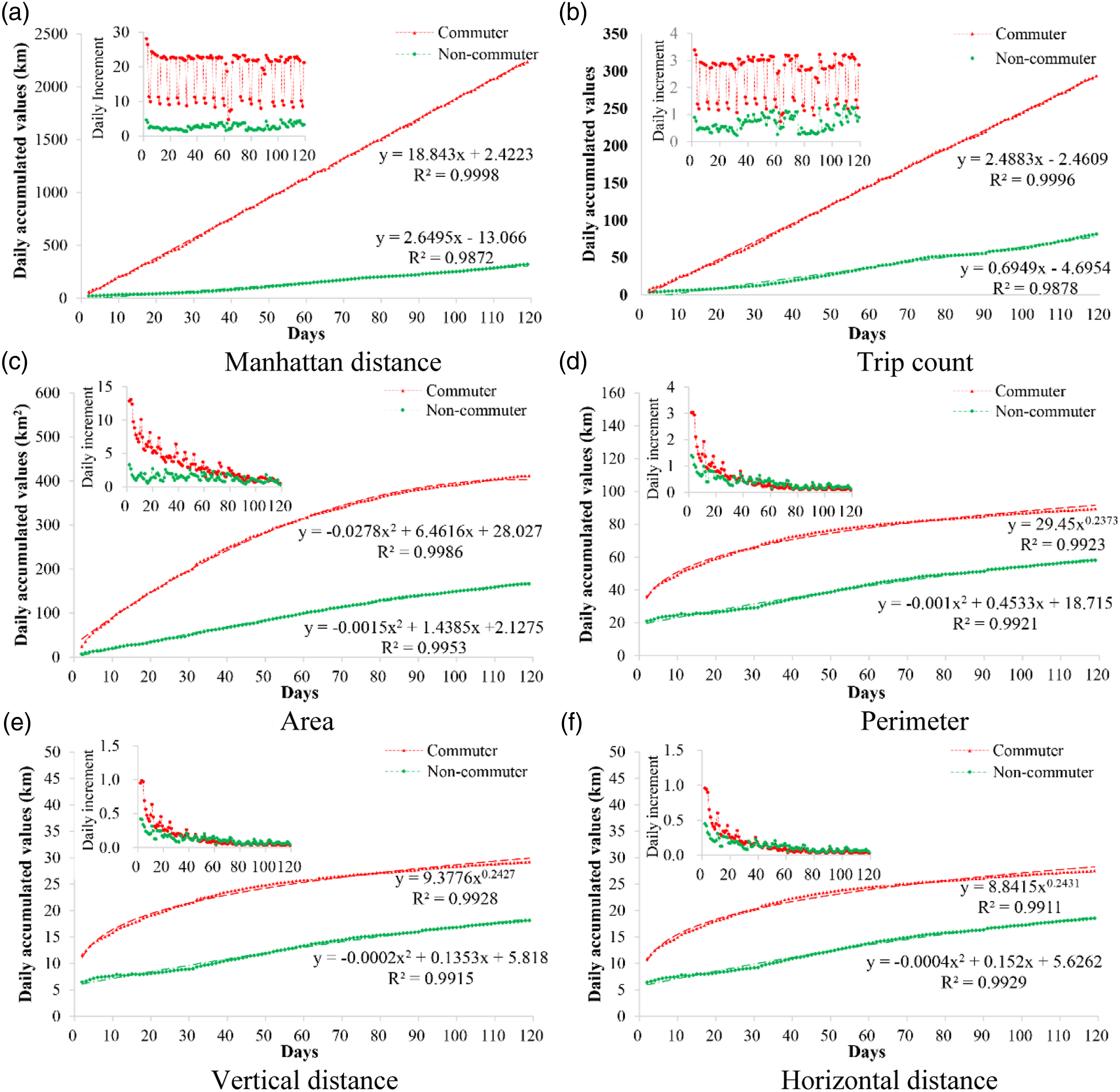

As shown in Figure 6 (a) and (b), the variation trends of travel distance and frequency perfectly grow linearly (R² > 0.98) with the accumulation of days. Meanwhile, the day-to-day variations of these two features experience a non-negative rate with periodic fluctuation. The ever-growing trends of these two features are interpretable, since a smart card holder will always increase his/her travel distances or trip counts by generating more journeys in the life span.

As shown in Figure 6 (c) to Figure 6 (f), area and the other three features involving space coverage are found to grow at a declining rate from the perspective of day-to-day variability. When it comes to day-accumulated variability, these features are better explained by either Power or Bivariate polynomial functions. The Power coefficients of perimeter, vertical/horizontal distance of commuters all range from 0 to 1, while the coefficients of $x^{2}$ of the Bivariate polynomial functions are negative for the rest space-coverage features. These fitting performances demonstrate that, a progressive decreasing of marginal increases emerges in these space-coverage features for both commuters and non-commuters. Each space-coverage feature, though increasing at varying speeds every day, will reach a summit ultimately, since its increasing rate gradually declines day by day. One probable explanation is that the maximum value of space coverage is limited by the size of a transit network. The above finding is consistent with a fact that farther places would be less interacted due to distance impedance.

Discussions and Conclusions

This paper explores variability in travel patterns for two groups of passengers over time. Unlike previous studies which mined day-to-day variability or worked on small-scale datasets, our research is conducted on a big smart card dataset generated by over 3.3 million passengers across 120 days. Day-to-day variability and day-accumulated variability are both investigated based on feature series involving space coverage, travel distance and travel frequency, with an aim to explore how, and to which extent, passengers in either category vary their travel patterns. The main findings and potential implications are summarized below.

(1) Temporal variability of travel patterns significantly differs, comparing commuters versus non-commuters and weekdays versus weekends. Particularly, on a daily basis, commuters travel 5.85 times longer and 2.50 times more frequently than non-commuters on weekdays, but cover less area. The opposite patterns occur on weekends, especially on Saturday. Trips generated in the ‘North-South’ direction are 1.45 times long as those generated in the orthogonal direction, where richer social resources can be found for commuters on weekdays, as well as for non-commuters on weekends. Commuters are less influenced by day of week or month of year, compared to non-commuters, due to more fixed travel routines. Yet, Friday is another story, when passengers in either type prefer to join entertainment activities with covering long distances and wide area.

Obviously, passengers in different types are confirmed to present distinct distributions of day-to-day variability in travel patterns. These distinctions can be used in our extension work to segment passengers into more specific subtypes. Moreover, the distinctions may serve as a basis to conduct personalized price differences for commuters and non-commuters on a day-to-day level, to balance their travel demands. But how it works needs an in-depth discussion in our future work.

(2) The temporal evolution curves of the six features, as shown in Figure 6, present two distinct types of variation rules for all passengers. The first is related to a linear growing of travel distance and frequency over time, while the second is related to a global convergence of space-coverage features which can be explained by either Power or Bivariate polynomial functions. These two patterns indicate that passengers have the tendency to travel long, yet cover a limited space in a long run.

Rules in the former type have been widely adopted in transit oriented development (TOD) in Beijing in the past five decades. Though TOD presents advantages in accelerating urbanization, it would bring a side effect on an unbalanced development of neighbourhoods in suburbs, where less social resources are injected, such as jobs, education or medical care. The convergent expansion in space coverage, instead, allows an enforcement of neighbourhood oriented development (NOD) implemented on the basis of TOD. So that land use functions could be injected with more diversity in each neighbourhood, especially in those neighbourhoods located in the ‘East-West’ direction in Beijing, to create more opportunities. Local governments could also launch preferential policies, for example, reducing taxes for enterprises, or decentralizing government-funded institutions, to attract more social resources in less developed suburbs.

Several limitations exist in this paper. Firstly, space coverage mentioned in the Build Temporal Series of Features to Characterize Variability in Travel Patterns section is measured by drawing a convex hull along stations visited by passengers, without considering their temporal variations simultaneously. It could be solved in the future by developing a space-time prism, rather than a convex hull, to capture space coverage. Besides, travel distance is now characterized by the Manhattan distance with considering that Beijing transit network is rectangular-shaped in the core, but less so farther out. Thus, it would be essential to combine it with other metrics in the future to better describe passengers’ travel distances. Secondly, when monthly variations are discussed, we only focus on weather, rather than other seasonal events such as holidays or festivals, which can also trigger variability in travel to large groups of passengers. This would be discussed as an extension of this work. Thirdly, passengers are only clustered into two classical types, that is, commuters and non-commuters, in this paper, with considering an easy validation of the derived results via priori knowledge. With such a rich data set, it will be interesting to cluster passengers into more specific subtypes, to explore vivid variability patterns in the future. Yet, how to validate potential results needs a further consideration. Finally, variability in travel patterns is assumed to be affected by temporal elements in this paper, without considering other influencing factors like incomes, genders and careers, which also require an in-depth analysis in the future. Yet, there is still a long way to go before we finish collecting these factors in large sample sizes automatically, which are hardly recorded via smart card data currently.

Supplemental Material

Supplemental Material - Exploring temporal variability in travel patterns on public transit using big smart card data

Supplemental Material for Exploring temporal variability in travel patterns on public transit using big smart card data by Xia Zhao, Mengying Cui and David Levinson in Environment and Planning B: Urban Analytics and City Science.

Footnotes

Declaration of conflicting interests

The author(s) declared no potential conflicts of interest with respect to the research, authorship, and/or publication of this article.

Funding

The author(s) disclosed receipt of the following financial support for the research, authorship, and/or publication of this article: This work was supported in part by China postdoctoral science foundation [grant number 2021M690332]; the Basic scientific research foundations for Municipal Universities [grant number X21061]; the National Natural Science Foundation of China [grant number U1811463, 61632006, 52172301, 62072015,5170080357]; the National Key R&D Program of China [grant number: 2021YFB2601200]; and the Beijing Social Science Foundation [grant number: 21GLA010].

ORCID iDs

Xia Zhao

Mengying Cui

David Levinson

Supplemental Material

Supplemental Material for this article is available online.

Notes

References

Arthur

Vassilvitskii

(2007) k-means++: The advantages of careful seeding. In: Proceedings of the 18th Annual ACM-SIAM Symposium on Discrete Algorithms, New Orleans Louisiana, January 7–9, 2007, pp. 1027–1035.

Briand

Come

Trepanier

, et al. (2017) Analyzing year-to-year changes in public transport passenger behaviour using smart card data. Transportation Research Part C: Emerging Technologies 79: 274–289.

Chu

K K

(2015) Two-year worth of smart card transaction data–extracting longitudinal observations for the understanding of travel behaviour. Transportation Research Procedia 11: 365–380.

Dharmowijoyo

Susilo

Y O

Karlstrom

(2016) Day-to-day variability in travellers’ activity-travel patterns in the Jakarta metropolitan area. Transportation 43(4): 601–621.

Dharmowijoyo

Susilo

Y O

KarlstroM

(2018) On complexity and variability of individuals' discretionary activities. Transportation 45: 177–204.

Fan

Khattak

(2008) Urban form, individual spatial footprints, and travel: Examination of space-use behavior. Transportation Research Record: Journal of the Transportation Research Board 2082: 98–106.

Fotheringham

O’Kelly

(1989) Spatial Interaction Models: Formulations and Applications. Dordrecht: Kluwer Academic Publishers, volume 1.

Gonzalez

Hidalgo

Barabasi

(2008) Understanding individual human mobility patterns. Nature 453: 779–782.

Han

Kamber

Pei

(2012) Data Mining: Concepts and Techniques. 3rd edition. USA: Morgan Kaufmann Publishers, pp. 364–368.

10.

Hasanzadeh

Czepkiewicz

Heinonen

, et al. (2019) Beyond geometries of activity spaces: a holistic study of daily travel patterns, individual characteristics, and perceived wellbeing in helsinki metropolitan area. Journal of Transport and Land Use.

11.

Huang

Levinson

Wang

, et al. (2018) Tracking job and housing dynamics with smartcard data. Proceedings of the National Academy of Sciences 115(50): 12710–12715.

12.

Huang

Levinson

Wang

, et al. (2019) Job-worker spatial dynamics in Beijing: Insights from smart card data. Cities 86: 83–93.

13.

Jarv

Ahas

Witlox

(2014) Understanding monthly variability in human activity spaces: a twelve-month study using mobile phone call detail records. Transportation Research Part C: Emerging Technologies 38: 122–135.

14.

Kandt

Leak

(2019) Examining inclusive mobility through smartcard data: What shall we make of senior citizens’ declining bus patronage in the West Midlands? Journal of Transport Geography 79: 102474.

15.

Kieu

Bhaskar

Chung

(2015) Passenger segmentation using smart card data. IEEE Transactions on Intelligent Transportation Systems 16: 1537–1548.

16.

Kitamura

Yoshii

Yamamoto

(2009) The Expanding Sphere of Travel Behaviour Research: Selected Papers from the 11th International Conference on Travel Behaviour Research. Bingley, UK: Emerald Group Publishing.

17.

Kumar

Tan

Steinbach

, et al. (2018) Introduction to Data Mining. 2nd Edition. London, UK: Pearson Education.

18.

Lee

Davis

Yoon

, et al. (2016) Activity space estimation with longitudinal observations of social media data. Transportation 43: 955–977.

19.

Leung

Zhao

(2016) Uncertainty analysis of space-time prisms based on the moment-design method. International Journal of Geographical Information Science 30: 1336–1358.

20.

Liu

Wen

, et al. (2017) Understanding commuting patterns using transit smart card data. Journal of Transport Geography 58: 135–145.

21.

Wang

, et al. (2013) Mining smart card data for transit riders’ travel patterns. Transportation Research Part C: Emerging Technologies 36: 1–12.

22.

Medina

Arturo

(2018) Inferring weekly primary activity patterns using public transport smart card data and a household travel survey. Travel Behaviour and Society 12: 93–101.

23.

Misra

Bhat

(2000) Activity-travel patterns of non-workers in the san francisco bay area: exploratory analysis. Journal of the Transportation Research Board 1718(1): 43–51.

24.

Raux

Cornelis

(2016) Variability in daily activity-travel patterns: the case of a one-week travel diary. European Transport Research Review 8: 1–14.

25.

Schonfelder

Axhausen

(2003) Activity spaces: measures of social exclusion? Transport Policy 10(4): 273–286.

26.

Shan

Ferreira

Gonzalez

, et al. (2017) Activity-based human mobility patterns inferred from mobile phone data: a case study of Singapore. IEEE Transactions on Big Data 3(2): 206–219.

27.

Susilo

Axhausen

(2014) Repetitions in individual daily activity-travel-location patterns: a study using the Herfindahl-Hirschman Index. Transportation 41(5): 995–1011.

28.

Wen

Liu

, et al. (2016) Beijing Transport Development Annual Report. Beijing: Beijing Transport Institute, pp. 25–28.

29.

Yildirimoglu

Limniati

Geroliminis

, et al. (2015) Investigating empirical implications of hysteresis in day-to-day travel time variability. Transportation Research Part C: Emerging Technologies 55: 340–350.

30.

Yong

Shen

, et al. (2018) Uncovering stable and occasional human mobility patterns: a case study of the Beijing subway. Physica A: Statistical Mechanics and Its Applications 492: 28–38.

31.

Yuan

Raubal

(2016) Analyzing the distribution of human activity space from mobile phone usage: an individual and urban-oriented study. International Journal of Geographical Information Science 30: 1594–1621.

32.

Zhang

Kang

Axhausen

, et al. (2018) Multi-day activity-travel pattern sampling based on single-day data. Transportation Research Part C Emerging Technologies 89: 96–112.

33.

Zhao

Zhang

Liu

, et al. (2019) Detecting pickpocketing gangs on buses with smart card data. IEEE Intelligent Transportation Systems Magazine 11(3): 181–199.

34.

Zhao

Cui

Levinson

(2020) Temporal Variations in Daily Activity Networks and Spaces Using Smart Card Data. Washington D.C: Transportation Research Board. paper ID 20-01216: 1-19.

35.

Zhong

Manley

Arisona

, et al. (2015) Measuring variability of mobility patterns from multiday smart-card data. Journal of Computational Science 9: 125–130.

36.

Zhou

Long

(2014) Jobs-housing balance of bus commuters in Beijing: Exploration with large-scale synthesized smart card data. Transportation Research Record 2418: 1–10.

Supplementary Material

Please find the following supplemental material available below.

For Open Access articles published under a Creative Commons License, all supplemental material carries the same license as the article it is associated with.

For non-Open Access articles published, all supplemental material carries a non-exclusive license, and permission requests for re-use of supplemental material or any part of supplemental material shall be sent directly to the copyright owner as specified in the copyright notice associated with the article.

0.00 MB

1.50 MB