Allocating synthetic population to a finer spatial scale: An integer quadratic programming formulation

Abstract

Agent-Based Models (ABMs) are being increasingly used to evaluate urban systems, urban policies and environmental impacts. One prerequisite for using the ABM framework consists of generating a synthetic population representative of the actual population, featuring the appropriate attributes with respect to model objectives. A precise spatial positioning of the synthetic population agents is often key to ensuring ABM modeling quality. This paper considers the problem of allocating synthetic population agents to a finer spatial scale. Such an allocation process is performed from a higher-level statistical area where a synthetic population can be generated, that is, a container statistical area (CSA), to several nested non-overlapping elementary statistical areas (ESAs), where only marginals are available. This allocation step relies not only on common attributes between CSA and ESA, but also on additional discriminatory attributes, that is, attributes of interest, estimated from external data sources. The case study examined herein is based on French census and fiscal data. Common attributes include eight socio-demographic variables, totaling 17 modalities. An additional attribute of interest, that is, income, has also been added. The allocation problem at hand is modeled as an integer quadratic programming problem. An exact algorithm is first applied to solve the problem; the applicability of this algorithm proves to be limited to small-size synthetic populations. A heuristic is proposed to handle the allocation of larger-size synthetic populations. Tests carried out on the case study show that this heuristic yields near-optimal solutions; it is also computationally efficient and may fulfill the needs of a majority of users.

Keywords

Spatialization finer scale allocation statistical areas synthetic population agents agent-based models integer quadratic programming problem

Introduction

Agent-Based Models (ABMs) are now widely used across a range of sectors, including urban planning, economic policy evaluation, environmental evaluation and transportation simulation. These models generally require detailed attributes of individuals and households in terms of socioeconomic characteristics. In order to perform an agent-based simulation, a necessary intermediate step therefore entails generating a simplified microscopic representation of the actual population, that is, a “synthetic population” derived from available data (Chapuis and Taillandier, 2019). Nevertheless, due to data limitation and for privacy reasons, no comprehensive dataset containing these detailed socio-demographic characteristics exists at a fine geographic scale.

In many ABM simulations, the behavior of synthetic agents is determined to a great extent by their attributes, as well as by their location. Hence, the spatial heterogeneity of agents’ characteristics must be taken into account with a granularity that depends on both model objectives and available spatial data (Zhu and Ferreira Jr, 2014; Chapuis et al., 2018). In many studies, the lack of geographic specificity has been identified as a major problem (Ji and Wan, 2021; Long and Shen, 2015; Anderson et al., 2014; Su et al., 2010; Nejad et al., 2021; Zhou et al., 2022). Simulated populations are often only allocated in census enumeration areas. These large area units do not provide sufficient spatial definition and, therefore, do not always allow for satisfactory analyses of transportation and urban planning (Thomson et al., 2018). More precise spatial information can dramatically improve the relevance and quality of analyses. For the purpose of obtaining a synthetic population at a finer spatial scale, two main approaches can be distinguished.

In the first approach, the synthetic population is directly generated at the lower level of elementary statistical areas. Three configurations of generation methods at lower level statistical areas can be distinguished: (1) Generation can be performed using a sample and marginals given at the lower level. However, due to privacy considerations, rarely a sample is given at such low level. Moreover, even if given, the sample is very limited which renders the generation of a representative population very complicated. Furthermore, difficult technical problems may arise for some generation methods when some attribute combinations are missing in the sample (Sun and Erath, 2015), notably the “zero-cell problem” (Guo and Bhat, 2007); (2) Generation is performed using a sample given at a higher-level statistical area combined with the marginals of lower level statistical area (Durán-Heras et al., 2018). However, as this sample is not specific to the elementary lower level area, there is no guarantee it is representative of its population (Nejad et al., 2021). Therefore, the representativeness of the generated synthetic population is affected; (3) Generation is performed with a sample-free method (Gargiulo et al., 2010; Barthelemy and Toint, 2013) using only marginals of lower level statistical area. Usually, marginal data are more readily available than sample data for small statistical areas, as they do not disclose personal information. The shortcoming of this approach is that important information for the generation process found in the sample, notably the joint relation between attributes, is lost. The representativeness of the generated synthetic population is severely diminished.

In the second approach, synthetic population agents are allocated to a finer spatial scale after the synthetic population is generated at a higher level. Two configurations of allocating to a finer spatial scale after the generation at a higher level can be distinguished: (1) Allocation of households to a finer scale is performed randomly. In many studies, the localization of synthetic population is limited to randomly assigning locations to synthetic households by selecting places among all available locations (e.g., assignment of home locations in Sallard et al. (2021)). Other studies try to control random assignment using counting information. Using land-use pre-processed satellite imagery and building geometries data, Chapuis et al. (2018) applied an areal interpolation method to disaggregate French census data and generate gridded prediction of population density at a finer scale (i.e., 30 m² raster cell). The synthetic individuals are then randomly assigned to cells with computed density constraints. However, this allocation process only controls for number of individuals or households; (2) Aggregate data (i.e., marginals) given for smaller areas contained in the larger areas, where the sample is given and the synthetic population is generated, are used to improve the precision of synthetic agents spatial positions. To our knowledge, few studies have applied this approach. Harada and Murata (2017) proposed a method that relies on marginals provided at finer scale units by Japanese administration. They generate a synthetic population on a city scale using a simulated annealing method and then assign each household to a district of the city. In a first step, they randomly assign each synthetic household according to the number of households by family type and the number of family members in each district. In a second step, they randomly select two households (same family type and same number of members) of two distinct districts and exchange them. Using district population statistics by sex and age, they evaluate this new solution and repeat this procedure as long as necessary. However, this approach only considers two variables for refining synthetic population allocation. Moreover, it can have a very high computational complexity, and can be applied to problems with limited size.

This paper proposes a method that aims to allocate synthetic population of households to a finer spatial scale after the synthetic population is generated at a higher level.

For this purpose, we rely on aggregate data (i.e., marginals) given for smaller areas contained in the larger area. We believe this approach of allocating synthetic agents spatial positions to a fine scale to be the most appropriate for two main reasons: (1) on the one hand, the synthetic population can be generated at the level where the sample is given. This is the most appropriate option to obtain a representative synthetic population at the corresponding level. Note that sample data with detailed individual characteristics are usually available with a low spatial precision and are attached to relatively large areas; (2) on the other hand, aggregate data (i.e., marginals) given for smaller areas contained in the larger area, where the synthetic population is generated, can be used in order to perform data-driven allocation of agents to these smaller areas. This data-driven assignment of synthetic population households is expected to noticeably improve results compared to random assignments. Furthermore, the data configuration where sample data are attached to relatively large areas but aggregate data are available at lower nested areas is very common.

Our method that aims to allocate a synthetic population from a higher-level statistical area to finer scale areas, that is, several nested non-overlapping elementary statistical areas is generic. In order to allocate synthetic agents from a higher-level statistical area, that is, container statistical area (CSA), to finer level elementary statistical areas (ESAs), two types of attributes are used: common attributes and additional attributes of interest computed from external data sources. The common attributes are available at both the CSA and ESA levels, whereas the attributes of interest are indeed available at one of the two levels, but approximate values of these attributes can still be computed at the other level. In considering a case study based on French census and fiscal data, this allocation problem is modeled as an integer quadratic programming problem. An exact algorithm is first applied to solve the problem; however, the applicability of this algorithm is limited to small-size synthetic populations (e.g., in order to allocate 120 households to six lower level areas, the resolution time exceeds 5 hours). Hence, a heuristic is proposed to handle the allocation of large synthetic populations; this heuristic is computationally efficient and yields near-optimal solutions.

The remainder of this paper is organized as follows. The first section describes the problem and our case study. The second section then lays out the mathematical problem and introduces both the decision variables and parameters. The third section is devoted to presenting our solution approaches and their corresponding results. The fourth section discusses the results of our analyses and is followed by a conclusion offering perspectives on this paper.

Description of the problem and case study

General formulation of the household allocation problem

This paper tackles the problem of allocating households from a container statistical area (CSA) to several nested non-overlapping elementary statistical areas (ESAs). Two distinct geographic levels have thus been considered.

At the higher level, that is, the container statistical area level, adequate information is available to generate a synthetic population representative of the real population. Typically, a disaggregated dataset, representing a sample of the population is available. Such a sample is commonly referred to as an International Public Use Micro Sample (IPUMS) and provides numerous socio-demographic attributes of individuals or households such as age, gender, family composition, and household income.¹ From this sample, a synthetic population can be generated using adequate methods (Hermes and Poulsen, 2012; Yaméogo et al., 2021).

At the lower level, that is, elementary statistical areas level, only aggregate data on a number of household attributes (that may or may not be available at the higher level) are provided. The number of attributes accessible at the ESA level tends to be smaller than that at the CSA level. Three attribute configurations between the two levels can be distinguished:

1. Attributes common to both CSA and ESA;

2. Attributes only present in CSA;

3. Attributes only present in ESA.

In order to obtain a more accurate location of the population’s households, the synthetic households may be allocated from the CSA level to the ESA level. Each CSA household needs to be assigned to one and only one ESA. For this purpose, the common attributes at both CSA and ESA levels are used, that is, households are assigned to ESA while satisfying the aggregate values of the common ESA-level attributes.

Since all these attributes are considered to be well aligned, such a problem can be solved using the constraint programming paradigm (Rossi et al., 2008), whereby constraints are defined so as to ensure that the marginals of each ESA are satisfied during the household assignment step. A solution to this constraint satisfaction problem (CSP) consists of an assignment that satisfies all constraints (Freuder and Mackworth, 2006). The quality of this solution then depends on both the number and discriminatory nature (i.e., ability to differentiate households) of the common attributes. More specifically, if the number of common attributes is small and these attributes remain insufficiently discriminatory, constraint satisfaction can indeed yield multiple solutions. Moreover, the number of possible solutions can be significant.

Figure 1 illustrates an example of dispatching 13 synthetic households at the CSA level into four ESA. Five attributes are available at both levels: three common ones and two solely present at one of the two levels. The attributes common to both levels are:

1. Dwelling ownership status (owner, tenant in CSA) and dwelling ownership status marginals (number of owners, number of tenants in each ESA);

2. Type of dwelling (apartment, house in CSA) and type of dwelling marginals (number of apartments, number of houses in each ESA);

3. Dwelling status (social, private in CSA) and dwelling status marginals (number of social dwellings, number of private dwellings in each ESA).

Figure 1.

Illustration of the household allocation problem (1/2).

The two remaining attributes, that is, car ownership and household composition, are only present in the CSA and the ESA, respectively. This assignment procedure can be carried out while relying on just the common attributes: a solution consists of assignments capable of satisfying the marginals of each ESA.

As shown in Figure 1, by relying on the three common attributes, multiple solutions of this assignment problem are indeed possible. This example yields two solutions with a distinct distribution of households between ESA units (the dashed and dotted arrows indicate that households hh7 and hh9 can be allocated to either ESA 1 or ESA 2). In configurations with a high number of households, the number of possible solutions can be much greater and it may often become necessary to enrich either the synthetic population attributes (CSA level) or the marginal data attributes (ESA level) with those estimated from other data sources. These additional attributes would need to be more discriminatory than the already available ones and are called attributes of interest given that allocation algorithms use them to achieve a more refined classification of households. In our example, household composition is a specific attribute only present at the ESA level. However, the number of individuals can also be estimated for each synthetic household by means of external data sources (e.g., additional statistics on household composition). Adding this information to the synthetic population can lead to a unique solution for household assignment, as illustrated in Figure 2.

Figure 2.

Illustration of the household allocation problem (2/2).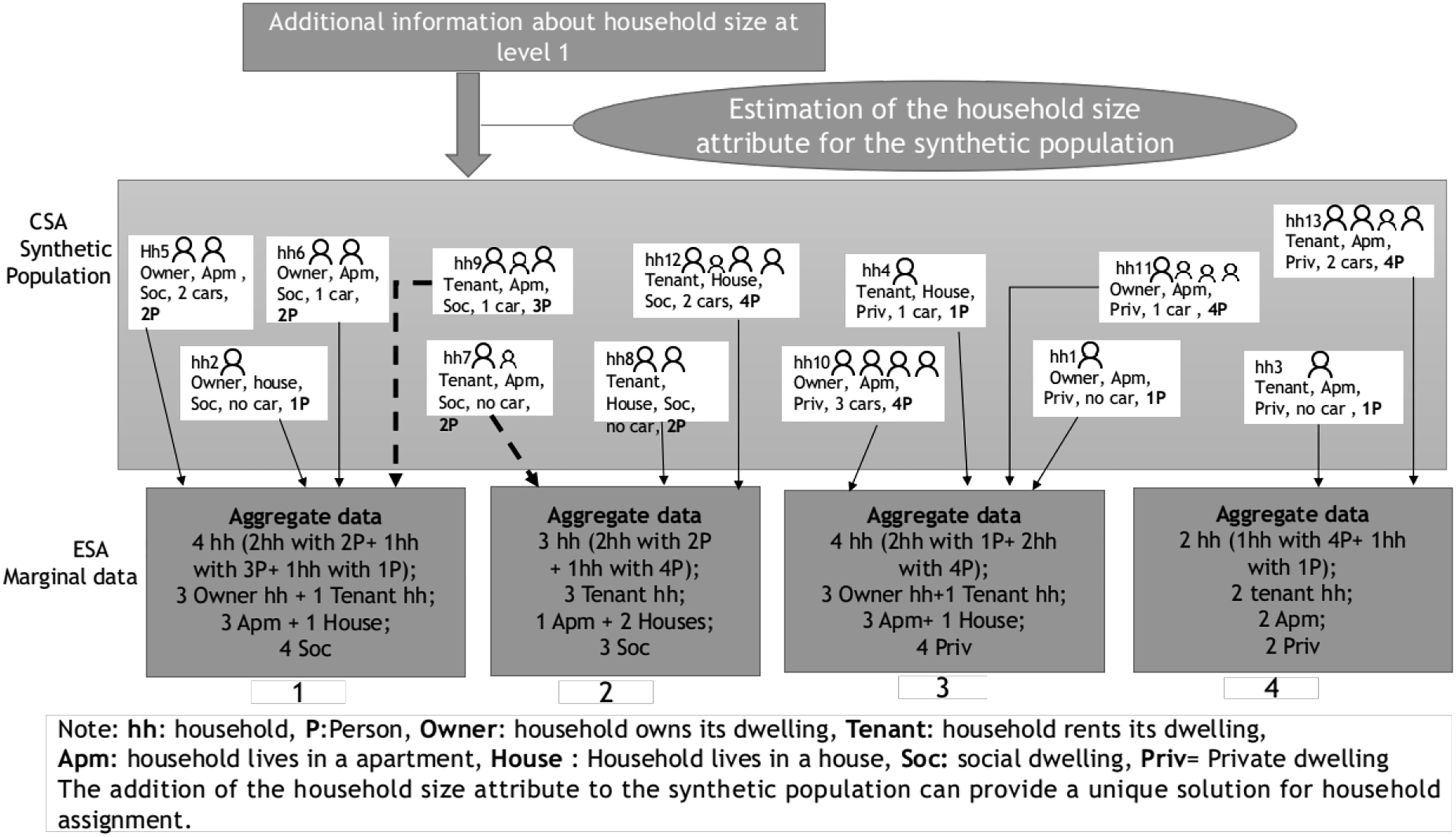

From a modeling perspective, since these attributes of interest are being estimated, they are probably not well aligned between the two levels. Hence, applying constraints to these attribute values, as is the case for the original common attributes, might be inappropriate. Instead, implementing one or several objective functions to use these attributes in assigning households to the ESA units would be suitable. These objective functions are used to minimize the gap of these attributes with respect to ESA marginals. Therefore, household assignment can be solved as a single or multi-objective optimization problem formulated on estimated attributes, along with constraints formulated on common variables.

This paper assigns households from a synthetic population within a container statistical area to several nested elementary statistical areas using both common and additional estimated attributes. The following section provides a detailed description of our case study.

Case study of allocation to a finer scale using French data

To illustrate the proposed method, we have used French data disseminated at two distinct geographic levels: IRIS (container statistical area) and grids (elementary statistical areas). We specifically worked with data from the city of Nantes, with these data being freely made available by the French National Institute of Statistics and Economic Studies (INSEE) Figure 3.

Figure 3.

Study area: city of Nantes (France).

Container statistical areas: IRIS units

IRIS (French acronym for “aggregated units for statistical information”) is a statistical zoning system for disseminating of intra-municipal data in the French population census. IRIS zones have clear boundaries that remain stable over the long term. Municipalities or cities with at least 5000 inhabitants are divided into several IRIS units; all municipalities not divided into IRIS units constitute an IRIS unit on their own.²

INSEE disseminates a representative sample of individuals and households at the IRIS scale. Each observation in the sample represents a unique individual, combined with the characteristics defining his or her person, household and main residence. This layout makes it possible to synthesize at the IRIS scale a realistic synthetic population of individuals associated with their households (also called a two-layered synthetic population) with multiple attributes. We thus began by generating a synthetic population of individuals and households from this sample.

Elementary statistical areas: Grid data

INSEE disseminates grid data corresponding to squares with sides ranging from 200 m to several kilometers. Grid units are smaller than IRIS units, and an IRIS can contain many non-overlapping grids. Grid decomposition respects the European directive INSPIRE enacted in 2007 (Bartha and Kocsis, 2011) and intended to harmonize spatial data across European countries in the aim of improved dissemination and interpretation of these data. Through a standard and compatible pattern, French grid data can be compared with German or Italian grid data (Darriau, 2020). French grid data mainly provide marginal information on the characteristics of households and their economic conditions. Similarly to IRIS-level data, grid data were collected during 2015.

Generation of a synthetic population

The city of Nantes sample (30% of the whole population) includes approximately 111,000 individuals residing in 62,000 households distributed over 97 IRIS. Sample data were collected from 2013 to 2017 and adjusted to the reference year of 2015. In the sample data, each observation represents an individual with personal characteristics (gender, age, profession, etc.), household characteristics (household size, family composition, etc.) and some characteristics of the dwelling (type of residence, size of the dwelling, etc.).

In addition to the sample data, aggregated data for the city of Nantes (at the IRIS level) are also available. These aggregated data contain the totals of certain socio-demographic attributes of the population (number of men and women in each IRIS, number of households by family composition, etc.). Based on the available data (large sample size, aggregated data) and according to the synthetic generation process described in Yaméogo et al. (2021), we selected the Hierarchical Iterative Proportional Fitting (HIPF) method proposed by Müller and Axhausen (2011) for generating a two-layered (or multi-level) synthetic population.³ Since the weights obtained with this method are not integer, we then applied the Truncate, Replicate Sample (TRS) approach (Lovelace and Ballas, 2013) to convert these decimal weights into integer weights in order to replicate individuals and households.⁴ For the synthetic population generation process, we considered nine control variables (i.e., variables for which aggregate data are available): five variables at the individual level and four variables at the household level (see Table A, Appendix A).

At the end of this process, we had derived a synthetic population corresponding to the actual population of Nantes: approximately 295,000 individuals residing in 157,000 households and 97 IRIS. Each household features a number of attributes (household size, family composition, date of dwelling completion, number of cars, etc.) as well as the socio-demographic attributes of household members (gender, age, profession, work status…).

However, one important attribute that cannot be generated in the synthetic population at the IRIS level is Income. For privacy reasons, household income is not available in the sample data, thus making it impossible to include it in the synthetic generation process. Nevertheless, it is possible to estimate, once the synthetic population has been generated, an income for each household at the IRIS level. Income constitutes an essential attribute when taking many social and economic aspects into account; it is also a highly discriminating attribute for households and, therefore, a key attribute of interest in the synthetic household allocation process. The income assignment process used will be described in the following subsection.

Household income estimation

The process of assigning income to synthetic households is performed using the FiLoSoFi (“localized disposable income system”) database provided by tax authorities. The income available in FiLoSoFi is actually an annual income per consumption unit (CU), that is, annual income divided by a weighting system that assigns a coefficient to each member of the household according to both household size and age of its members.⁵ By convention, all members of the same household are assigned the same income. For the city of Nantes, FiLoSoFi contains the deciles of the annual income distribution for the entire population along with certain specific variables, namely: number of persons, family composition, ownership status, and age of the reference person in the household.

In Yaméogo et al. (2021), a heuristic was proposed to assign an additional variable to a synthetic population when the aggregate data distribution is given in deciles. This heuristic combined Bayes’ theorem with the cross-entropy minimization algorithm and was successfully used herein to allocate an income to each of the 157,000 synthetic households living in the city of Nantes. The results were easy to compute and wound up being consistent with most of the deciles.

Summary of data present in both IRIS and grids

As previously explained, a synthetic population with both household and individual attributes is allocated from the IRIS level (container statistical areas) to the grid unit level (elementary statistical areas). These units are associated with household marginal attributes. Each IRIS unit contains many non-overlapping grids. The allocation process employed herein has been performed using two types of attributes:

1. Household attributes (not estimated) common to both IRIS and grids. These attributes are primarily related to household and dwelling characteristics;

2. An attribute of interest, namely, household income. In our original database, this attribute is only given at the grid level, that is, “total household income,” and moreover represents the aggregate income of all households living within the grid. From additional data sources (i.e., FiLoSoFi database), a corresponding attribute, that is, “household income,” can be estimated for each synthetic household at the IRIS level.

Table 1 summarizes both the common attributes and the estimated attribute of interest.

Table 1.

Attributes for synthetic population allocation at both the IRIS and grid levels.

Categories	Synthetic population Initial attributes	Harmonization of synthetic population attributes with grid marginal	Grid marginals
Household size	Single member	Single member	Number of single member households
	2 persons	2–4 members	Number of households between 2 and 4 members
	3 persons
	4 persons
	5 persons and more	5 persons and more	Number of households with 5 or more members
Household ownership status	Owner	Owner	Number of owner households
Household ownership status	Tenant	Tenant	Number of tenant households
Household composition	Single-parent	Single-parent	Number of single-parent households
	Single woman	Non-single parent	Number of non-single parent households
	Single man
	Couple without children
	Couple with children
	Complex household
Household economic status	Household in poverty	Household in poverty	Number of households in income poverty
Household economic status	Non-poor household	Non-poor household	Number of non-poor households
Household income	Simulated attribute (euros)	Simulated attribute (euros)	Total household income (euros)
Type of dwelling	House	House	Number of households living in a house
Type of dwelling	Apartment	Apartment	Number of households living in an apartment
Date of construction of the dwelling	Before 1919	Before 1945	Number of dwellings built before 1945
	Between 1919 and 1944	Before 1945	Number of dwellings built before 1945
	Between 1945 and 1970	Between 1945 and 1989	Number of dwellings built between 1945 and 1989
	Between 1971 and 1989	Between 1945 and 1989	Number of dwellings built between 1945 and 1989
	Between 1990 and 2005	Since 1990	Number of dwellings built since 1990
	Between 2006 and 2012
	Since 2013
Dwelling status	Social dwelling	Social dwelling	Number of social dwellings
Dwelling status	Non-social dwelling	Non-social dwelling	Number of non-social dwellings
Household	Household to assign	Household to assign	Number of households

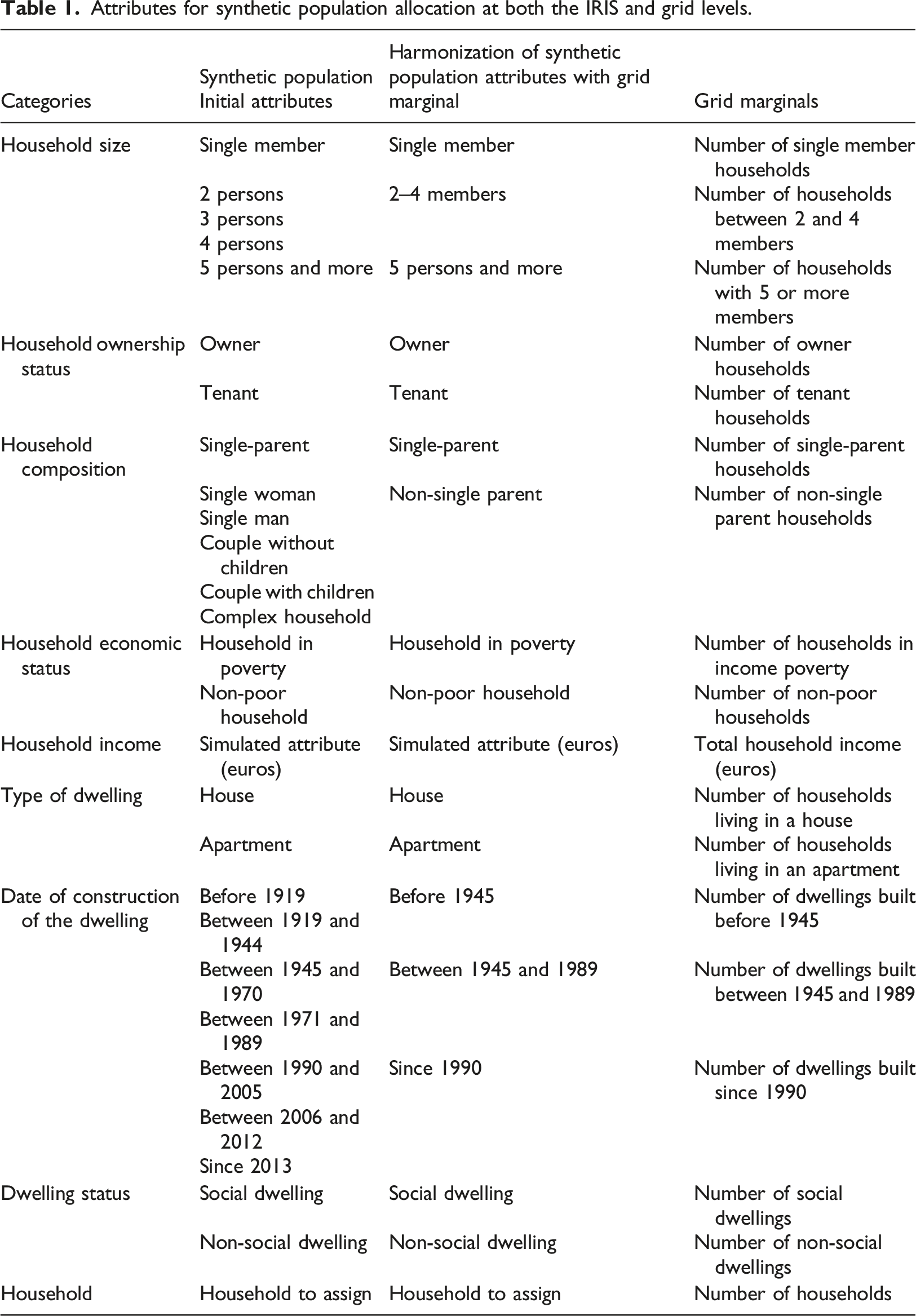
Common attributes include: household size, household ownership status, household composition, household economic status, household income, type of dwelling, date of construction of dwelling and dwelling status. These attributes are encoded as categorical variables of synthetic population agents at the IRIS level. The number of occurrence of modalities of these attributes is given at grid level. However, the modalities at IRIS and grid levels are not aligned perfectly. This can be seen in columns “Synthetic Population Initial attributes” and “Grid marginals” of Table 1. In order to align these attributes, modalities of the synthetic population at IRIS level are transformed as shown in column “Harmonization of synthetic population attributes with grid marginals” of Table 1. The attribute of interest, that is, is encoded as a real number at both the IRIS and grid levels. At the IRIS level, it represents the income of the corresponding household of the synthetic population, while at grid level, it represents the sum of households incomes of corresponding grid.

The next section provides a detailed description of our proposed allocation method.

Mathematical formulation of the household allocation problem

Decision variables and parameters

In order to model the synthetic population allocation, we first introduced, using the attribute information from Table 1, the following sets, indices, decision variables and parameters.

Sets and indices

Let J be the set of synthetic households: J = 1, 2, …, N_J;

Let I be the set of grids: I = 1, 2, …, N_I;

Each household j ∈ J is to be assigned to exactly one grid i ∈ I.

Decision variables

We define N_J × N_I decision variables, whereby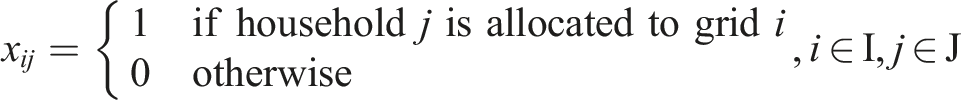

x_{i j} = {\begin{array}{l} 1 & if household j is allocated to grid i \\ 0 & otherwise \end{array}, i \in I, j \in J

Parameters

In order to be incorporated into the decision problem, attribute values shown in Table 1 are defined as parameters. Synthetic population households common attributes at IRIS level are transformed and encoded as binary parameters, each parameter representing a modality (e.g., single-parent household), and take the value 1 if household j exhibits the characteristic or 0 otherwise. The encoding of number of occurrence of modalities at grid level as well as the income attribute at both levels remain unchanged, values are simply assigned to corresponding parameters.

Hereafter, grid parameters are indicated in capital letters and household parameters in lower case.

NH_i: Number of households in grid i;

TINC_i: Total household income in grid i;

inc_j: Income of household j.

The other problem parameters are listed in Table 2.

Table 2.

List of the other problem parameters.

Description	IRIS household parameters	Grid marginal parameters
Household size/composition
Households between 2 and 4 members	s2_j	TS2_i
Households size >4	s5_j	TS5_i
Single-parent households	sp_j	TSP_i
Ownership
Owner	o_j	TO_i
House	h_j	TH_i
Dwelling type
Dwelling built before 1945	d45_j	TD45_i
Dwelling built since 1990	d90_j	TD90_i
Economic status
Social dwelling	so_j	TSO_i
Income poverty	p_j	TP_i

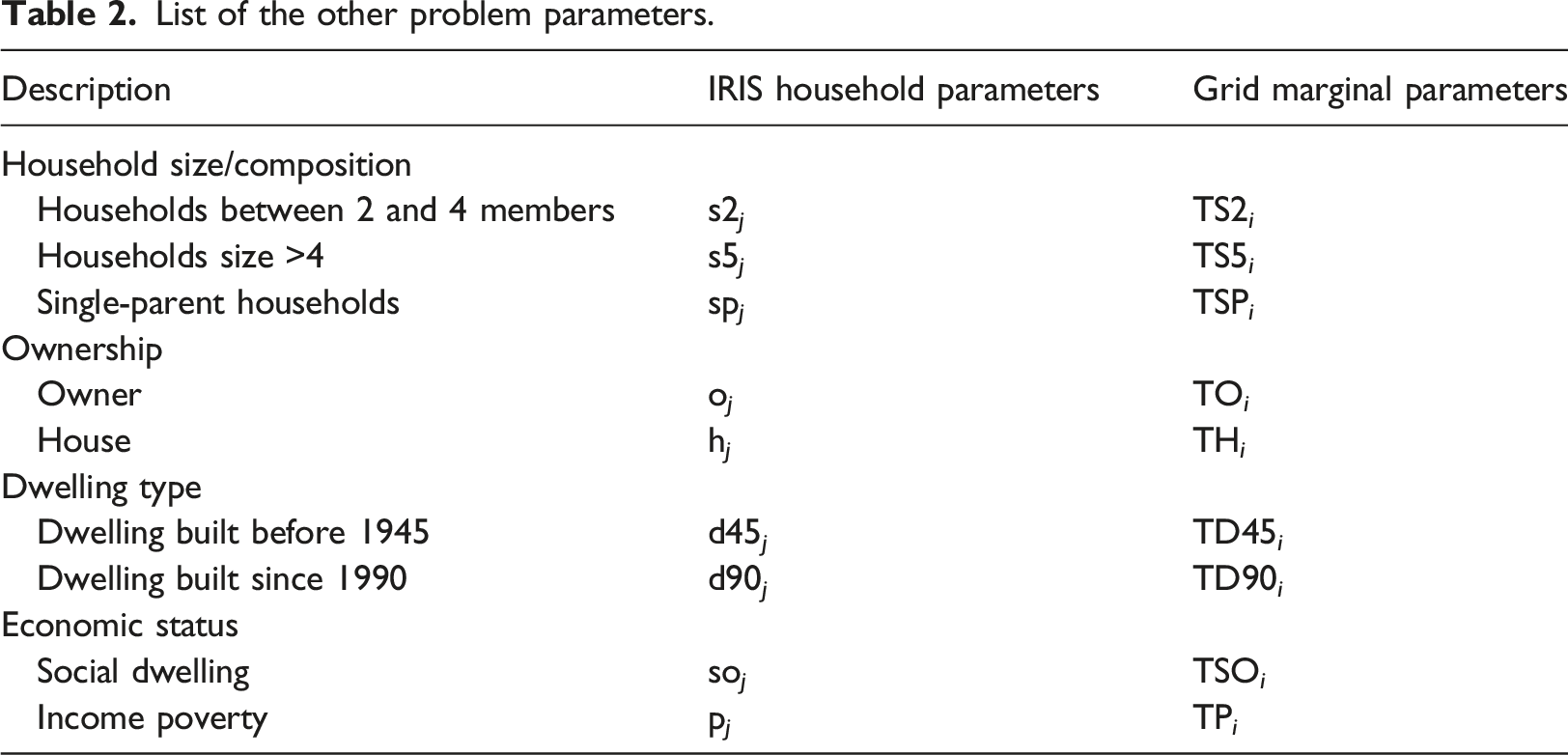
All household parameters in Table 2 are binary and take the value 1 if household j exhibits the characteristic or 0 otherwise. For example

S 2_{j} = {\begin{array}{l} 1 & if household j size is between 2 and 4 members \\ 0 & otherwise \end{array}

Objective function and constraints

As mentioned above, the parameter inc_j (income of household j) was estimated once the synthetic population had been generated. Therefore, the following equality 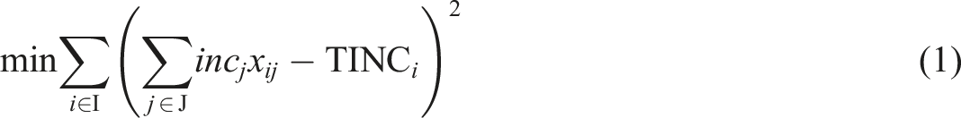$\sum_{j = 1}^{J} i n c_{j} x_{i j} = {TINC}_{i}$ is not necessarily respected. However, we are seeking an assignment of household j to a grid i such that the sum of incomes for the chosen assignments (i.e., x_i,j = 1) lies as close as possible to the total household income of the grid. This gap minimization can be modeled as an objective function. Moreover, the grid marginals of the other attributes (i.e., common attributes) can still be respected. For this purpose, a constraint modeling approach is appropriate. Given these considerations, the synthetic population allocation problem can be modeled as a single-objective optimization problem, yielding the following formulation

\min \sum_{i \in I} {(\sum_{j \in J} i n c_{j} x_{i j} - {TINC}_{i})}^{2}

(1)

subject to the following constraints

\sum_{i \in I} x_{i j} = 1, j \in J

(2)

\sum_{j \in J} x_{i j} = {NH}_{i}, i \in I

(3)

\sum_{j \in J} x_{i j} S 2_{j} = TS 2_{i}, i \in I

(4)

\sum_{j \in J} x_{i j} S 5_{j} = TS 5_{i}, i \in I

(5)

\sum_{j \in J} x_{i j} S p_{j} = {TSP}_{i}, i \in I

(6)

\sum_{j \in J} x_{i j} o_{j} = T 0_{i}, i \in I

(7)

\sum_{j \in J} x_{i j} h_{j} = {TH}_{i}, i \in I

(8)

\sum_{j \in J} x_{i j} d 45_{j} = TD 45_{i}, i \in I

(9)

\sum_{j \in J} x_{i j} d 90_{j} = TD 90_{i}, i \in I

(10)

\sum_{j \in J} x_{i j} S o_{j} = {TSO}_{i}, i \in I

(11)

\sum_{j \in J} x_{i j} p_{j} = {TP}_{i}, i \in I

(12)

x_{i j} \in {0,1}, i \in I, j \in J

(13)

equation (1) constitutes the objective function, while the other equations provide the constraints which can be classified into two types:

1. Validity constraints (equations (2) and (13)) that apply to for every household j ∈ J. These constraints express the fact that each household is assigned to exactly one grid.

2. Marginal-control constraints (equations (3) to (12)) that ensure that specific marginals (associated with common attributes) of each grid are being respected.

In the model formulation, the decision variables x_ij are binary; moreover, the objective function is quadratic and all constraints are linear. The model assumes the form of an integer quadratic programming problem which is characterized by a quadratic objective function to be minimized over a set of linear constraints and a share of binary bounded variables.

Integer quadratic programming problem

An integer quadratic programming problem (Billionnet and Elloumi, 2007; Del Pia et al., 2017) is a discrete optimization problem, a particular set of mathematical programming problems (Bierlaire, 2015). Discrete optimization problems are characterized by an objective function and a set of constraints where some or all of the decision variables are discrete and take integer values. Such problems arise in contexts where decisions are to be taken concerning entities that are indivisible. A particular case of discrete optimization problems is when variables are binary, taking only the values 0 or 1. A value 1 may refer to an action to be taken while the value 0 corresponds to an action not taken.

A discrete optimization problem is an integer linear programming problem if the objective function and the constraints are linear functions of the decision variables, and if all of its variables are restricted to take integer values. Integer linear programming problems where all the variables are restricted to take the values 0 or 1 are also called binary linear programming problems. Many classical optimization problems can be formulated as integer linear programming problems including the generalized assignment problem (Öncan, 2007), the knapsack problem (Salkin and De Kluyver, 1975), the set covering problem (Balas and Padberg, 1972) and the traveling salesman problem (Jünger et al., 1995). A harder to solve discrete optimization problem than linear integer problems is when the objective function and/or constraints are quadratic. A problem where the objective function is quadratic but constraints are linear is termed an integer quadratic programming problem. If the problem has any constraints containing a quadratic term, regardless of the objective function, the problem is termed an integer quadratically constrained programming problem.

Discrete optimization problems can be solved using exact methods or heuristics. The exact methods guarantee that an optimal solution is found if the algorithm terminates in a reasonable time. These methods include enumeration techniques, including the branch-and-bound procedure (Lawler and Wood, 1966) and cutting-plane techniques (Kelley, 1960). Due to the combinatorial nature of discrete optimization problems, exact methods may fail to identify the optimal solution in a reasonable amount of time. In this case, for practical purposes, a heuristic algorithm is used to identify quickly a good feasible solution, that is an approximation of the exact one. This heuristic can be problem-specific in order to solve the latter in a numerically efficient and robust manner.

Mathematical modeling of the synthetic population allocation problem yields an optimization problem with binary decision variables. The value of a given decision variable indicates whether corresponding household is assigned to corresponding grid or not. On this aspect, our problem is comparable to the well-known assignment problems (Burkard et al., 2012). These problems deal with the allocation of a number of agents to a number of tasks on one to one basis. The objective is to find the best assignment of agents to tasks, where the profit is maximum. They are commonly formulated as integer programming problems with binary decision variables.

Integer programming problems with a quadratic objective function have arisen in numerous scientific fields. Some recent applications where the problem is modeled this way include topological state estimation in water distribution systems (Díaz et al., 2018), embedded hybrid model predictive control (Bemporad and Naik, 2018), optimal freewheeling control of a heavy-duty vehicle (Held et al., 2020), optimization of a district energy system (Blackburn et al., 2019), generation units maintenance in combined heat and power integrated systems (Sadeghian et al., 2020), and smart home energy management (Killian et al., 2018).

Problem-Solving

This section presents both the approach and results of solving this allocation problem. For this purpose, a simulated dataset, representative of the French data configuration has been used. This dataset allows for an enhanced evaluation of computational performance and solution quality of the resolution algorithms. Two solution approaches were tested. Despite application of an integer quadratic programming solver, this approach was not suitable for large-size problems since the computational time varied exponentially with the number of households. Consequently, a heuristic has been proposed (see second part of this section).

Construction of a simulated dataset

In order to test the computational performance and solution quality of resolution algorithms, we created datasets representative of available French data. In the city of Nantes, the maximum number of households in an IRIS equals roughly 4200; therefore, our initial pool contained 6000 synthetic households. Each of these households possesses the attributes listed in Table 1. We then drew a specific number of households from this pool in order to constitute a simulated IRIS (while controlling their size) of Nantes. For the purposes of our test, we also considered each simulated IRIS to be divided into six nested non-overlapping grids, numbered from 1 to 6.

In order to control problem size as well as the expected results, we adopted the following approach:

1. Step 1: We first assigned each household of the pool’s 6000 households to a grid; this assignment was carried out so as to have heterogeneous grids in terms of both size and composition. For example, some grids have a high total household income, while others have a large number of social dwellings. The six grids are thus representative of the heterogeneity of Nantes area grids. In our simulated dataset, grids 1, 2, 3, 4, 5, and 6 contain, respectively, 1,332; 540; 1,518; 1,044; 840; and 726 households.

2. Step 2: Once all 6000 households had been allocated to the grids is done, we then randomly selected a number of households in each grid. For example, for grid 1, we selected X₁ households among the 1332 (X₁ ≤ 1, 332), X₂ households among the 540 (X₂ ≤ 540) for grid 2 and so on for all the other grids. At the end of this process, we had a simulated IRIS of X households (with X = X₁ + X₂ + X₃ + X₄ + X₅ + X₆), where each household had been assigned to one of the six grids.

3. Step 3: We computed the grid marginals (corresponding to the household attributes) for the X_i households selected in Step 2 across the six grids. The marginals of each grid were obtained by summing the values of the attributes of its households. Hence, the marginals in grid 1 were obtained by summing the values of the attributes of the X₁ households, including the income attribute. Table 3 summarizes the grid marginals of the largest simulated IRIS, composed of all of 6000 households in the pool (i.e., X₁ = 1, 332, X₂ = 540, …, X₆ = 726).

4. Step 4: Once the marginals of the grids had been computed, the household affiliation with the grids could be neglected (in order to obtain the same configuration as the original data). The solver was subsequently used to perform this allocation step.

Table 3.

Grid marginals of the largest simulated IRIS composed of all 6000 households.

Parameters	Grids (i)
Parameters	Grid 1	Grid 2	Grid 3	Grid 4	Grid 5	Grid 6
N	1332	540	1518	1044	840	726
TINC	61 083 330	33 507 367	66 008 163	50 128 765	46 573 815	24 869 918
TINC_by_N^a	45 858.35	62 050.68	43 483.64	48 016.06	55 445.02	34 256.08
TP	333	67	269	247	107	134
TS2	573	277	668	553	487	249
TS5	174	54	58	107	43	6
TO	53	341	474	40	461	143
TSP	275	33	189	226	79	58
TH	23	282	174	47	448	75
TD45	20	226	14	29	50	59
TD90	258	103	628	155	129	154
TSO	1233	28	769	986	241	332

^aTINC/N.

Two key features of such a simulated dataset can be underscored: (1) the problem size is controlled, therefore the computational performance and algorithm resolution limits can be tested; and (2) the exact result of the objective function minimization is known (i.e., equal to zero). This latter feature is due to the fact that the income marginal was originally computed as the sum of individual synthetic household incomes. In actuality, this equality is not respected and this minimization will not result in a zero solution because income is in fact an estimated attribute. However, the advantage of relying on this simulated input data configuration is to test result accuracy when the resolution algorithm is not exact; this is particularly important since computationally efficient algorithms are not exact ones.

Using the simulated input dataset, we then proceeded to assign X households (X = X₁ + X₂ + X₃ + X₄ + X₅ + X₆), according to the computed grid parameters. We were thus able to perfectly measure the accuracy of the results and test the computational performance of the solver in order to determine the problem size, that is, the “number of households,” that can potentially be solved. Table 3 reports the initial grid parameters.

Integer quadratic programming solver

Matrix form of the integer quadratic programming problem

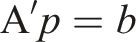
In order to use an integer quadratic programming solver efficiently, our integer quadratic programming problem, as formulated in equations (1) to (13), must be written in the following matrix form (Bonami et al., 2018)

\min \frac{1}{2} x^{T} Q x + c^{T} x

(14)

A x = b

(15)

x_{i j} \in {0,1} i \in I, j \in J

(16)

1. equation (14), with $c \in ℝ^{n}$ and Q (n × n real symmetric matrix), represents the matrix form of the quadratic objective function in equation (1);

2. equation (15), with matrix $A \in ℝ^{m \times n}$ and the right-hand side vector $b \in ℝ^{m}$ , represents the set of linear constraints given in equations (2) to (12);

3. equation (16) specifies that decision variables are indeed binary.

After modeling our problem in this matrix form by specifying the four components Q, c, A, b, the implementation proved to be relatively simple in a dedicated solver. In this paper, we used IBM ILOG CPLEX Optimization Studio solver, a commercial software to model and solve optimization problems (Laborie et al., 2018).⁶ CPLEX is a conventional and powerful tool for solving linear or integer optimization problems. The present allocation procedure was run with R (version 4.0.3) and IBM ILOG CPLEX Optimization Studio version 20.1.0.0. We specifically chose the R package “Rcplex,” which is an R interface to CPLEX solvers for linear, quadratic and (linear and quadratic) integer programs.⁷ This package requires IBM ILOG CPLEX libraries and headers. To test the integer quadratic programming problem resolution, a simulated dataset was used.

Performance of the IQP problem resolution

We started with a simulated IRIS containing a small number of households and then gradually increased the size gradually. For each simulated IRIS with a given number of households, we ran the solver 15 times. The resolution was carried out on a Windows 10 Professional machine, Intel(R) Core (TM) i7-8665U CPU @ 1.90 GHz, 2.11 GHz and 16 GB of RAM. The solver was able to compute the optimal solution (minimization yields zero using simulated data) for the following simulated IRIS sizes:

1. For a size of X = 30 households (X₁ = 7, X₂ = 4, X₃ = 6, X₄ = 3, X₅ = 6, X₆ = 4), the solver was able to solve the integer quadratic programming problem in less than a second;

2. For X = 60 households (X₁ = 17, X₂ = 8, X₃ = 14, X₄ = 5, X₅ = 12, X₆ = 4), the resolution time varied between 1.4 min and 2 h;

3. For X = 120 households (X₁ = 32, X₂ = 17, X₃ = 21, X₄ = 15, X₅ = 25, X₆ = 10), the resolution time exceeded 5 hours.

A large number of households cannot be assigned within reasonable time period with an integer quadratic programming solver. The heuristic yielding a practical and faster solution is proposed below.

Heuristic for a large-scale problem

Relaxation of the integer quadratic programming problem and selection of synthetic population from the computed probability

The two main limitations associated with the algorithm used for solving IQP problem are

1. The complexity of finding optimal solution as integer-valued decision variables are required;

2. The large number of decision variables that leads to memory problem when constructing the objective matrix Q in equation (14).

We propose a heuristic that removes these limitations.

1. The decision variables become real numbers between 0 and 1. These variables, p_ij, are interpreted as probabilities for household j to belong to Grid i.

2. We replace the households that have the same common attributes and close incomes by an average household whose income is the average income of the replaced households (the other common attributes remain the same). A new attribute, N_j, whose value is equal to the number of replaced households is added. The set of average households is denoted J’.

The new objective function is rewritten as follows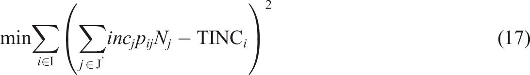

\min \sum_{i \in I} {(\sum_{j \in J^{'}} i n c_{j} p_{i j} N_{j} - {TINC}_{i})}^{2}

(17)

subject to the following constraints

\sum_{i \in I} p_{i j} = 1, j \in J^{'}

(18)

\sum_{j \in J^{'}} p_{i j} N_{j} = {NH}_{i}, i \in I

(19)

\sum_{j \in J^{'}} p_{i j} S 2_{j} N_{j} = TS 2_{i}, i \in I

(20)

\sum_{j \in J^{'}} p_{i j} S 5_{j} N_{j} = TS 5_{i}, i \in I

(21)

\sum_{j \in J^{'}} p_{i j} S p_{j} N_{j} = {TSP}_{i}, i \in I

(22)

\sum_{j \in J^{'}} p_{i j} o_{j} N_{j} = T 0_{i}, i \in I

(23)

\sum_{j \in J^{'}} p_{i j} h_{j} N_{j} = {TH}_{i}, i \in I

(24)

\sum_{j \in J^{'}} x_{i j} d 45_{j} N_{j} = TD 45_{i}, i \in I

(25)

\sum_{j \in J^{'}} x_{i j} d 90_{j} N_{j} = TD 90_{i}, i \in I

(26)

\sum_{j \in J^{'}} x_{i j} S o_{j} N_{j} = {TSO}_{i}, i \in I

(27)

\sum_{j \in J^{'}} p_{i j} p_{j} N_{j} = {TP}_{i}, i \in I

(28)

p_{i j} \in [0,1], i \in I, j \in J^{'}

(29)

In the same way as in the previous sections, these equations lead to the following compact equations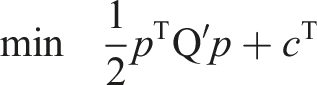

\min \frac{1}{2} p^{T} Q^{'} p + c^{T}

A^{'} p = b

p_{i j} \in [0,1] i \in I, j \in J^{'}

(30)

\sum_{j \in J^{'}} x_{i j} = 1, i \in I

(31)

The resulting problem then entails a quadratic programming (QP) problem (Gill and Wong, 2015) and is easier to solve than an integer quadratic programming problem.

Since we estimated probabilities, we then performed assignment in the grids by drawing households according to their estimated probabilities. However, since this approach is an heuristic and does not yield an exact solution, results should be carefully examined. We thus proceeded with 1000 different draws to analyze the gap between the obtained grid parameter values when the households were drawn and actual values. However, there is only one synthetic population assigned to the grids. The following proposed algorithm serves to pick out one distributed synthetic population from among the 1000 generated.

1. The user defines a tolerance, noted tol, around the attribute of interest; in the present case, for total income (TINC), we chose 5%. An initial selection consists of selecting the distributed synthetic population whose total income for each grid lies in the interval [(1 − tol) × TINC, (1 + tol) × TINC], with TINC being the actual income of the grid. This step defines a first set of synthetic populations.

2. For each distributed synthetic population belonging to this set, a criterion is calculated; this criterion measures the gap between all marginals computed with the population (except for the income) and the actual grid parameters. In our case study, we opted to calculate this gap by means of an absolute value.

3. The selected synthetic population is the one able to minimize this criterion.

The heuristic described in this section was also implemented with R programming language. The QP problem is solved using CPLEX connected to R with the “Rcplex” package.⁸

Performance of the heuristic algorithm

To assess the performance of the proposed method, we compared the average values of grid parameters for all 1000 draws (Table 4) with the initial grid parameters (Table 3). We also display in Table 4, the average values of grid parameters generated by the very popular Iterative Proportional Fitting (IPF) approach. For each Grid i, the IPF solution is computed by

1. Setting an initial weight of one at each household of the initial sample;

2. Letting IPF algorithm to modify this initial weight in order to fulfill the marginals of Grid i excepted for the total income which is a continuous variable which cannot be processed by the algorithm;

3. Interpreting these updated weights as a probability and then following the same procedure as for the heuristic, that is, a sampling is carried out with 1000 draws to pick up a final population.

Table 4.

Average grid parameter values after 1000 draws (Heuristic vs IPF).

Parameters	Grids (i) Heuristic/IPF
Parameters	Grid 1	Grid 2	Grid 3	Grid 4	Grid 5	Grid 6
N	1332/1327	540/537	1518/1525	1044/1044	840/838	726/729
TINC × 10³	61 095/59 642	33 482/33 405	66 019/66 048	50 110/49 203	46 586/47 993	24 876/25 877
TINC_by_N^a	45 859/44 937	62 042/62 158	43 484/43 321	48 021/47 148	55 449/57 274	34 256/35 493
TP	333/330	67/66	269/270	247/247	107/109	134/135
TS2	573/561	277/283	668/679	553/543	487/485	249/256
TS5	174/167	54/54	58/61	107/105	43/49	6/6
TO	53/55	341/343	474/474	40/41	461/455	143/145
TSP	275/267	33/37	189/190	226/222	79/83	58/61
TH	23/27	282/275	174/177	47/56	448/440	75/74
TD45	20/24	226/214	14/15	29/37	50/50	59/57
TD90	258/255	103/107	628/621	155/154	129/135	154/154
TSO	1233/1225	28/29	769/766	986/984	241/247	332/337

^aTINC/N.

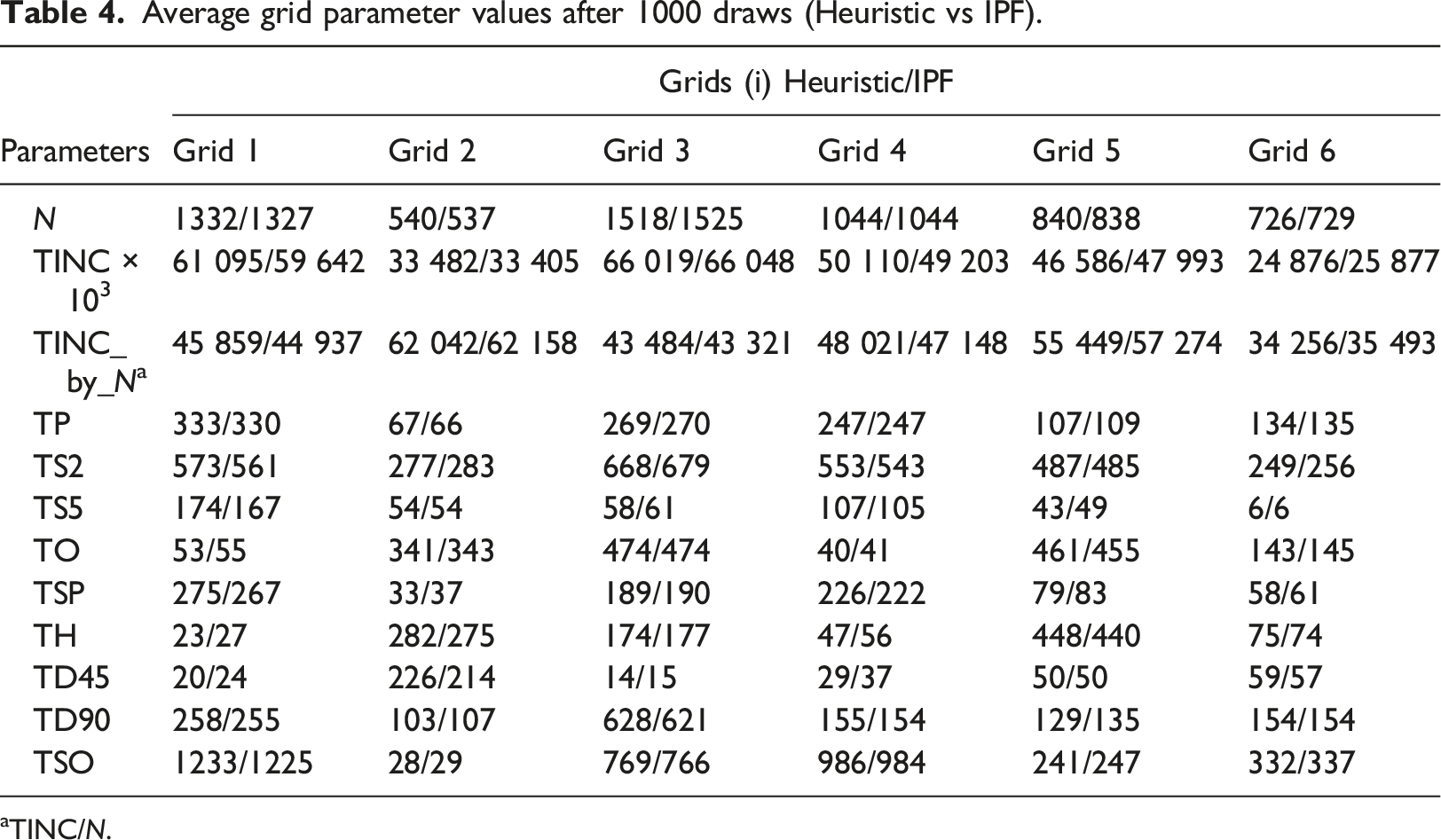
Note that there is no assurance that a household is assigned to only one Grid.

Table 3 and Table 4 are nearly identical, meaning no bias has entered into our process. The heuristic algorithm seems to outperform the IPF algorithm when regarding the average values of our attribute of interest, that is, household income (TINC_by_N). Concerning the other marginals, the heuristic and the IPF method provide similar results. The IPF algorithm resolution time was 2 s for the 6000 households of the largest simulated IRIS (Table 3). It is better than the computing time of the heuristic (43 s) on this specific problem.⁹ However, the heuristic is independent of the size of the population. A case study with more than 1,000,000 households has thus been simulated to demonstrate the applicability of the method to a large-scale synthetic population problem. For this problem, the resolution by the heuristic is largely more rapid (2 s to compare to 12 min) than the resolution by the IPF algorithm which depends on the size of the population. Details of this case study and results are given in the Appendix C.

Figure 4 displays the average values obtained after 1000 draws for each parameter and each grid.

Figure 4.

Error bars with confidence intervals showing the average grid parameter values after 1000 draws (Heuristic).

The dashed lines in Figure 4 represent the actual grid values for each parameter (reported in Table 3). The average values and actual values are nearly identical. For each grid and each parameter, the actual value always lies in the 95% confidence interval. The length of the confidence intervals is also quite small, implying that a large proportion of the sampled distributed synthetic populations exhibits values close to the actual values.

Our findings suggest that the relaxed optimization problem solver yields overall results consistent with all initial grid parameters.

Table 5 measures the absolute differences between the solution computed by the heuristic using the minimum criteria and the true solution (initial grid parameters) for the number of household and for each marginals. For each parameter, the second line displays explicitly the difference between the output of the heuristic and the true value. Only very small differences were found. The largest differences occur for: 25 households (TO, Grid 5), 19 households (TO, grid 2), and 14 households (TO, grid 3). However, these differences must be put into perspective because they relate to parameters with large numbers, that is, respectively, 461, 341, and 1518.

Table 5.

Absolute and relative differences between the solution computed by the heuristic with the minimum criteria and the initial grid parameters.

Parameters	Grids (i) computed/Actual marginals
Parameters	Grid 1	Grid 2	Grid 3	Grid 4	Grid 5	Grid 6
N	1 335/1 332	550/540	1 504/1 518	1 047/1 044	840/840	724/726
N	3 (0.2%)	10 (1.8%)	14 (−0.9%)	3 (0.2%)	0 (0%)	2 (−0.2%)
TP	338/333	71/67	265/269	239/247	115/107	129/134
TP	5 (1.5%)	4 (5.9%)	4 (−1.4%)	8 (−3.2%)	8 (7.4%)	5 (−3.7%)
TS2	571/573	277/277	668/668	556/553	490/487	245/249
TS2	2 (−0.3%)	0 (0%)	0 (0%)	3 (0.5%)	3 (0.6%)	4 (−1.6%)
TS5	188/174	54/54	55/58	99/107	44/43	2/6
TS5	14 (8%)	0 (0%)	3 (−5.1%)	8 (−7.4%)	1 (2.3%)	4 (−66.6%)
TO	56/53	360/341	476/474	35/40	436/461	149/143
TO	3 (5.6%)	19 (5.5%)	2 (0.4%)	5 (−12.5%)	25 (−5.4%)	6 (4.1%)
TSP	272/275	35/33	188/189	219/226	86/79	60/58
TSP	3 (−1%)	2 (6%)	1 (−0.5%)	7 (−3%)	7 (8.8%)	2 (3.4%)
TH	26/23	286/282	183/174	33/47	437/448	84/75
TH	3 (13%)	4 (1.4%)	9 (4.1%)	14 (−29.7%)	11 (−2.4%)	9 (12%)
TD45	16/20	230/226	8/14	35/29	43/50	66/59
TD45	4 (−20%)	4 (1.7%)	6 (−42.8%)	6 (20.6%)	7 (−14%)	7 (11.8%)
TD90	260/258	107/103	632/628	152/155	136/129	140/154
TD90	2 (0.7%)	4 (3.8%)	4 (0.6%)	3 (−1.9%)	7 (5.4%)	14 (−9%)
TSO	1228/1233	26/28	760/769	992/986	251/241	332/332
TSO	5 (−0.4%)	2 (−7.1%)	9 (−1.1%)	6 (0.6%)	10 (4.1%)	0 (0%)

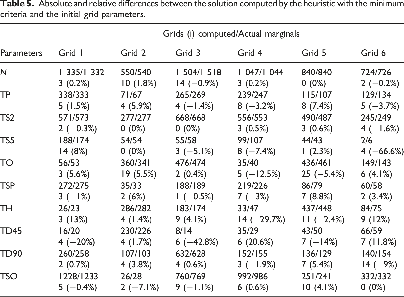
In order to evaluate the robustness and applicability of our method to real case studies, we have carried additional tests. We relied on data provided for the city of Nantes. We identified several cases, and performed synthetic population agents allocation from CSA to several ESA by using the heuristic. Results show that the heuristic is efficient in ensuring small differences between resulting ESA marginals after allocation and original values of these marginals (see supplementary material).

Conclusion

This paper has modeled the allocation of a synthetic population to a finer spatial scale. This allocation process was performed originating from a container statistical area (CSA), where adequate data for population generation is available, to several nested non-overlapping elementary statistical areas (ESA), where only aggregate data is available. For this purpose, two types of attributes were used: common attributes available at both levels and additional attributes of interest only available at one level but able to be computed from external data sources at the other level. This data configuration is commonly found in datasets provided by national statistical institutes. The methodology developed herein is thus general in scope and can be easily applied in many contexts.

In our specific application, the allocation challenge was modeled as a single-objective, integer quadratic programming problem. The objective function was a minimization of the gap in the attribute of interest between the observed value obtained by allocating the population to ESA units and the actual marginal of this attribute at each ESA. Constrains were applied to the other attributes, common to both synthetic population and ESA marginals. The attribute of interest considered herein was income, and common attributes included household size, household composition, and type of dwelling.

A classical algorithm was first used to find an exact solution to the problem. It was shown that the applicability of this algorithm is limited to small-size synthetic populations. Next, a heuristic was proposed and implemented on a simulated case study, that is, allocating 6000 households to six ESA units. By means of this heuristic, an efficient resolution (i.e., quick resolution times) and near-optimal results could be achieved.

Several improvements to the algorithm will be proposed in future studies. The most straightforward extension of the proposed approach is to consider the case where several attributes of interest can be computed and used for allocating households, thus yielding a multi-objective optimization problem whose resolution requires further study. Another challenge to be addressed is the case where one ESA unit straddles several CSA units, in which case such an ESA unit would need to be split into several sub-units corresponding to the originating CSA units. However, this process would still involve computing the marginals of the newly defined sub-units.

Lastly, allocating households to a fine-grained spatial area is of utmost importance in ABM. Any improvement to the spatial allocation process of a synthetic population at a finer scale will greatly benefit transportation and urban planning practitioners. Such advances are especially vital for the analysis and modeling of issues like management of environmental and urban systems. Since our methodology has been applied to a common data configuration, it is suitable for use in allocating synthetic populations within a wide array of case studies.

Supplemental Material

Supplemental Material - Allocating synthetic population to a finer spatial scale: An integer quadratic programming formulation

Supplemental Material for Allocating synthetic population to a finer spatial scale: An integer quadratic programming formulation by Boyam Fabrice Yameogo, Pierre Hankach, Pierre-Olivier Vandanjon, and Pascal Gastineau in Environment and Planning B: Urban Analytics and City Science

Footnotes

Declaration of conflicting interests

The author(s) declared no potential conflicts of interest with respect to the research, authorship, and/or publication of this article.

Funding

The author(s) received no financial support for the research, authorship, and/or publication of this article.

ORCID iDs

Boyam Fabrice Yameogo

Pierre Hankach

Pierre-Olivier Vandanjon

Supplemental Material

Supplemental material for this article is available online.

Notes

Appendix A

Table A.

Individual and household-level control variables.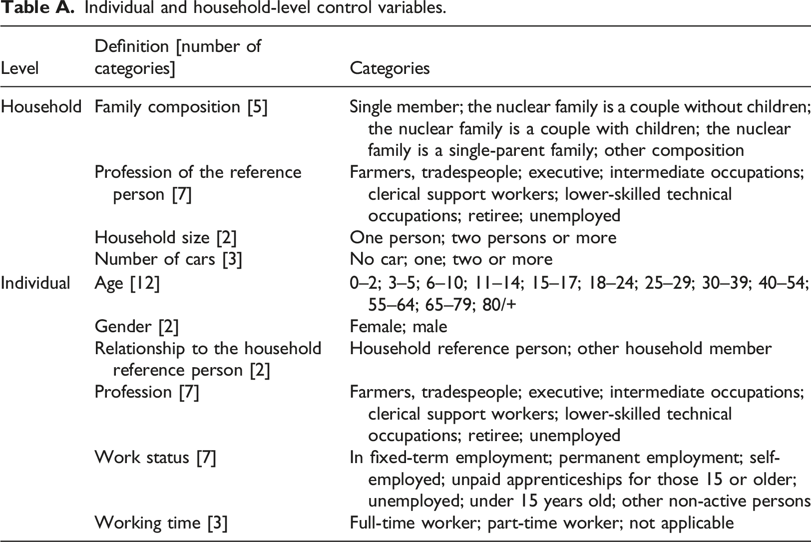

Level	Definition [number of categories]	Categories
Household	Family composition [5]	Single member; the nuclear family is a couple without children; the nuclear family is a couple with children; the nuclear family is a single-parent family; other composition
	Profession of the reference person [7]	Farmers, tradespeople; executive; intermediate occupations; clerical support workers; lower-skilled technical occupations; retiree; unemployed
	Household size [2]	One person; two persons or more
	Number of cars [3]	No car; one; two or more
Individual	Age [12]	0–2; 3–5; 6–10; 11–14; 15–17; 18–24; 25–29; 30–39; 40–54; 55–64; 65–79; 80/+
	Gender [2]	Female; male
	Relationship to the household reference person [2]	Household reference person; other household member
	Profession [7]	Farmers, tradespeople; executive; intermediate occupations; clerical support workers; lower-skilled technical occupations; retiree; unemployed
	Work status [7]	In fixed-term employment; permanent employment; self-employed; unpaid apprenticeships for those 15 or older; unemployed; under 15 years old; other non-active persons
	Working time [3]	Full-time worker; part-time worker; not applicable

Appendix B

Figure A.

Workflow of the case study.

Description

In order to demonstrate the independence of the heuristic to the number of households, the size of the city of Nantes is artificially augmented from 157,000 to 1 million (1,103,529 exactly) households. These households have to be dispatched to four artificial ESA which are built by merging neighboring Iris (see Figure (B)). Figure B.

Four artificial ESA.

Table (B) presents the comparison between the outputs of the heuristic the ESA marginals for the total income, the income divided by the number of households and for each marginal. A second line displays the difference between the outputs of the heuristic and the marginals in absolute and in percentage. As each ESA represents a large part of the city, the social segregation is not large; the income by household (TINC/N) varies from 40 161 to 50 561 €. The marginals are well respected (the difference in percentage is below 1%).

Results

Table B.

Marginals from a large-scale population (>1,000,000 households) spatialized by the heuristic versus ESA marginals.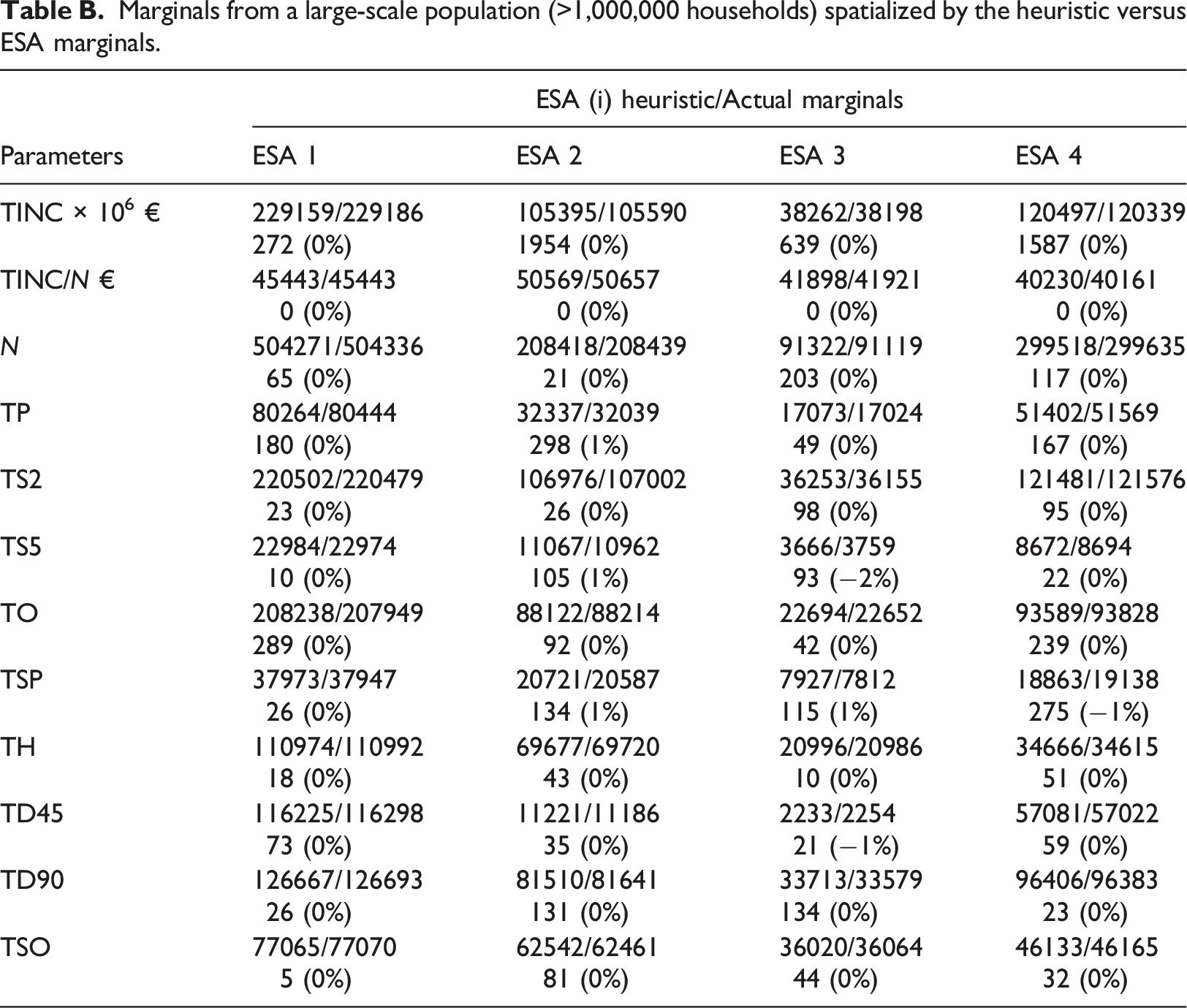

Parameters	ESA (i) heuristic/Actual marginals
Parameters	ESA 1	ESA 2	ESA 3	ESA 4
TINC × 10⁶ €	229159/229186	105395/105590	38262/38198	120497/120339
TINC × 10⁶ €	272 (0%)	1954 (0%)	639 (0%)	1587 (0%)
TINC/N €	45443/45443	50569/50657	41898/41921	40230/40161
TINC/N €	0 (0%)	0 (0%)	0 (0%)	0 (0%)
N	504271/504336	208418/208439	91322/91119	299518/299635
N	65 (0%)	21 (0%)	203 (0%)	117 (0%)
TP	80264/80444	32337/32039	17073/17024	51402/51569
TP	180 (0%)	298 (1%)	49 (0%)	167 (0%)
TS2	220502/220479	106976/107002	36253/36155	121481/121576
TS2	23 (0%)	26 (0%)	98 (0%)	95 (0%)
TS5	22984/22974	11067/10962	3666/3759	8672/8694
TS5	10 (0%)	105 (1%)	93 (−2%)	22 (0%)
TO	208238/207949	88122/88214	22694/22652	93589/93828
TO	289 (0%)	92 (0%)	42 (0%)	239 (0%)
TSP	37973/37947	20721/20587	7927/7812	18863/19138
TSP	26 (0%)	134 (1%)	115 (1%)	275 (−1%)
TH	110974/110992	69677/69720	20996/20986	34666/34615
TH	18 (0%)	43 (0%)	10 (0%)	51 (0%)
TD45	116225/116298	11221/11186	2233/2254	57081/57022
TD45	73 (0%)	35 (0%)	21 (−1%)	59 (0%)
TD90	126667/126693	81510/81641	33713/33579	96406/96383
TD90	26 (0%)	131 (0%)	134 (0%)	23 (0%)
TSO	77065/77070	62542/62461	36020/36064	46133/46165
TSO	5 (0%)	81 (0%)	44 (0%)	32 (0%)

Computing time

The computing time is 2 s for the heuristic on a computer with the following main features: Intel(R) Xeon(R) E−2236 CPU @ 3.40 GHz, 32Go. By way of comparison, on the same problem, the computing time for the IPF algorithm is 12 min.

References

Anderson

Guikema

Zaitchik

, et al. (2014) Methods for estimating population density in data-limited areas: Evaluating regression and tree-based models in Peru. Plos One 9(7): e100037.

Balas

Padberg

(1972) On the set-covering problem. Operations Research 20(6): 1152–1161.

Bartha

Kocsis

(2011) Standardization of geographic data: The european inspire directive. European Journal of Geography 2(2): 79–89.

Barthelemy

Toint

(2013) Synthetic population generation without a sample. Transportation Science 47(2): 266–279.

Bemporad

Naik

(2018) A numerically robust mixed-integer quadratic programming solver for embedded hybrid model predictive control. IFAC-PapersOnLine 51(20): 412–417.

Bierlaire

(2015) Optimization: Principles and Algorithms. Number BOOK. EPFL Press.

Billionnet

Elloumi

(2007) Using a mixed integer quadratic programming solver for the unconstrained quadratic 0-1 problem. Mathematical Programming 109(1): 55–68.

Blackburn

Young

Rogers

, et al. (2019) Dynamic optimization of a district energy system with storage using a novel mixed-integer quadratic programming algorithm. Optimization and Engineering 20(2): 575–603.

Bonami

Lodi

Zarpellon

(2018) Learning a classification of mixed-integer quadratic programming problems. In: International Conference on the Integration of Constraint Programming, Artificial Intelligence, and Operations Research. Springer, pp. 595–604.

10.

Burkard

Dell’Amico

Martello

(2012) Assignment Problems: Revised Reprint. SIAM.

11.

Chapuis

Taillandier

(2019) A brief review of synthetic population generation practices in agent-based social simulation SSC2019, Social Simulation Conference.

12.

Chapuis

Taillandier

Renaud

, et al. (2018) Gen*: A generic toolkit to generate spatially explicit synthetic populations. International Journal of Geographical Information Science 32: 1194–1210.

13.

Darriau

(2020) Les données carroyées, des outils et méthodes innovants pour percevoir la réalité des territoires. Courrier des statistiques 5: 53–73. Retrievied 13 April 2021: https://www.insee.fr/fr/information/5008679?sommaire=5008710

14.

Del Pia

Dey

Molinaro

(2017) Mixed-integer quadratic programming is in NP. Mathematical Programming 162(1): 225–240.

15.

Díaz

Mínguez

González

(2018) Topological state estimation in water distribution systems: Mixed-integer quadratic programming approach. Journal of Water Resources Planning and Management 144(7): 04018026.

16.

Durán-Heras

García-Gutiérrez

Castilla-Alcalá

(2018) Comparison of iterative proportional fitting and simulated annealing as synthetic population generation techniques: Importance of the rounding method. Computers, Environment and Urban Systems 68: 78–88.

17.

Freuder

Mackworth

(2006) Constraint satisfaction: An emerging paradigm. Handbook of Constraint Programming. Elsevier, 2, pp. 13–27.

18.

Gargiulo

Ternes

Huet

, et al. (2010) An iterative approach for generating statistically realistic populations of households. Plos One 5(1): e8828.

19.

Gill

Wong

(2015) Methods for convex and general quadratic programming. Mathematical Programming Computation 7(1): 71–112.

20.

Guo

Bhat

(2007) Population synthesis for microsimulating travel behavior. Transportation Research Record 2014(1): 92–101.

21.

Harada

Murata

(2017) Projecting households of synthetic population on buildings using fundamental geospatial data. SICE Journal of Control, Measurement, and System Integration 10(6): 505–512.

22.

Held

Flärdh

Roos

, et al. (2020) Optimal freewheeling control of a heavy-duty vehicle using mixed integer quadratic programming. IFAC-PapersOnLine 53(2): 13809–13815.

23.

Hermes

Poulsen

(2012) A review of current methods to generate synthetic spatial microdata using reweighting and future directions. Computers, Environment and Urban Systems 36(4): 281–290.

24.

Wan

(2021) A Novel Method for Socioeconomic Data Spatialization. Spatial Statistics.100501.

25.

Jünger

Reinelt

Rinaldi

(1995) The traveling salesman problem. Handbooks in Operations Research and Management Science 7: 225–330.

26.

Kelley

Jr (1960) The cutting-plane method for solving convex programs. Journal of the Society for Industrial and Applied Mathematics 8(4): 703–712.

27.

Killian

Zauner

Kozek

(2018) Comprehensive smart home energy management system using mixed-integer quadratic-programming. Applied Energy 222: 662–672.

28.

Laborie

Rogerie

Shaw

, et al. (2018) IBM ILOG CP optimizer for scheduling. Constraints 23(2): 210–250.

29.

Lawler

Wood

(1966) Branch-and-bound methods: A survey. Operations Research 14(4): 699–719.

30.

Long

Shen

(2015) Population spatialization and synthesis with open data Geospatial Analysis to Support Urban Planning in Beijing. Springer, pp. 115–131.

31.

Lovelace

Ballas

(2013) ‘truncate, replicate, sample’: A method for creating integer weights for spatial microsimulation. Computers, Environment and Urban Systems 41: 1–11.

32.

Müller

Axhausen

(2011) Hierarchical IPF: Generating a Synthetic Population for switzerland. European Regional Science Association.

33.

Nejad

Erdogan

Cirillo

(2021) A statistical approach to small area synthetic population generation as a basis for carless evacuation planning. Journal of Transport Geography 90: 102902.

34.

Öncan

(2007) A survey of the generalized assignment problem and its applications. INFOR: Information Systems and Operational Research 45(3): 123–141.

35.

Rossi

van Beek

Walsh

(2008) Chapter 4 constraint programming. In: van Harmelen

Lifschitz

Porter

(eds), Handbook of Knowledge Representation, volume 3 of Foundations of Artificial Intelligence. Elsevier, pp. 181–211.

36.

Sadeghian

Moradzadeh

Mohammadi-Ivatloo

, et al. (2020) Generation units maintenance in combined heat and power integrated systems using the mixed integer quadratic programming approach. Energies 13(11): 2840.

37.

Salkin

De Kluyver

(1975) The knapsack problem: a survey. Naval Research Logistics Quarterly 22(1): 127–144.

38.

Sallard

Balać

Hörl

(2021) An open data-driven approach for travel demand synthesis: an application to são paulo. Regional Studies, Regional Science 8(1): 371–386.

39.

M-D

Lin

M-C

Hsieh

H-I

, et al. (2010) Multi-layer multi-class dasymetric mapping to estimate population distribution. Science of the Total Environment 408(20): 4807–4816.

40.

Sun

Erath

(2015) A bayesian network approach for population synthesis. Transportation Research Part C: Emerging Technologies 61: 49–62.

41.

Thomson

Kools

Jochem

(2018) Linking synthetic populations to household geolocations: a demonstration in Namibia. Data 3(3): 30.

42.

Yaméogo

Gastineau

Hankach

, et al. (2021) Comparing methods for generating a two-layered synthetic population. Transportation Research Record 2675(1): 136–147.

43.

Zhou

Basu

, et al. (2022) Creating spatially-detailed heterogeneous synthetic populations for agent-based microsimulation. Computers, Environment and Urban Systems 91: 101717.

44.

Zhu

Ferreira

Jr (2014) Synthetic population generation at disaggregated spatial scales for land use and transportation microsimulation. Transportation Research Record 2429(1): 168–177.

Supplementary Material

Please find the following supplemental material available below.

For Open Access articles published under a Creative Commons License, all supplemental material carries the same license as the article it is associated with.

For non-Open Access articles published, all supplemental material carries a non-exclusive license, and permission requests for re-use of supplemental material or any part of supplemental material shall be sent directly to the copyright owner as specified in the copyright notice associated with the article.

0.00 MB

0.17 MB