Agglomeration effects as spatially embedded social interactions: identifying urban scaling beyond metropolitan areas

Abstract

Agglomeration is the tell-tale sign of cities and urbanization. Identifying and measuring agglomeration economies has been achieved by a variety of means and by various disciplines, including urban economics, quantitative geography, and regional science. Agglomeration is typically expressed as the non-linear dependence of many different urban quantities on city size, proxied by population. The identification and measurement of agglomeration effects is of course dependent on the choice of spatial units. Metropolitan areas (or their equivalent) have been the preferred spatial units for urban scaling modeling. The many issues surrounding the delineation of metropolitan areas have tended to obscure that urban scaling is principally about the measurable consequences of social and economic interactions embedded in physical space and facilitated by physical proximity and infrastructure. These generative processes obviously must exist in the spatial subcomponents of metropolitan areas. Using data for counties and urbanized areas in the United States, we show that the generative processes that give rise to scaling effects are not an artifact of metropolitan definitions and exist at smaller spatial scales.

Keywords

gross domestic product counties urban areas metropolitan areas social mixing

Introduction

Agglomeration effects are the tell-tale sign of cities and urbanization. These effects are empirically grounded observations of systematic changes in average socioeconomic performance, land-use patterns, and infrastructure characteristics of all cities as functions of their population size. Agglomeration is typically expressed as the non-linear dependence of different urban quantities on city size, proxied by population. There are many urban attributes that have been characterized in this way, from economic performance to crime, measures of invention to land uses, and many more (Strange, 2008). Urban scaling theory draws on insights from urban economics, economic geography, and regional science and shares with these disciplines a common explanation for the existence and development of cities as resulting from the interplay between centripetal and centrifugal “forces” (Colby, 1933; Fujita, Krugman and Venables, 1999; Isard, 1956). The nucleation forces result from the socioeconomic advantages of spatially concentrated and interacting human populations after accounting for the associated costs (Glaeser, 2011). These agglomeration effects constitute the foundational concepts for explaining the formation and persistence of cities (Duranton and Puga, 2004; Rosenthal and Strange, 2001; Storper, 2013).

The urban scaling framework provides articulating arguments for the long-standing recognition in economics, sociology, and anthropology that population size is a determinant of many socioeconomic features of human settlements (Carneiro, 2000; Johnson and Earle, 2000). The scaling approach builds on research in urban economics, geography, and complex systems that identified relationships between urban scale and economic productivity, innovation rates, energy use, and infrastructure needs (Bloom, Canning and Fink, 2008; Glaeser, Sacerdote and Scheinkman, 2003; Nordbeck, 1971). Such relations are known as scaling relations, and the systematic study of such relationships has come to be known as urban scaling. Over the past decade, a formal theory of urban scaling has emerged (Bettencourt, 2013). The core of this theory is a process of concentration of social, economic, and political interactions in space and time, subject to constraints imposed by environmental conditions, technology, and institutions (Bettencourt, 2014). These processes are the micro-level foundations upon which the explanatory framework is built. These processes are very general, and as a result, the urban scaling framework applies to settlements in any context provided they are physical settings for social interactions. Urban Scaling Theory has been applied across many urban systems throughout the world (from the USA, China, Brazil, India, European nations, South Africa, and more) and across history using archeological and anthropological evidence (Lobo et al., 2020).

The identification of agglomeration effects is dependent upon the choice of spatial units; the measurement of phenomena revealed through the aggregation of spatial data can vary significantly depending upon the spatial scale (Gehlke and Biehl, 1934; Openshaw, 1983; Wong, 2009). The study of urban agglomeration effects has focused on functional cities, definitions of urban areas that include place of residence and place of work within the same boundary for the majority of its inhabitants. In the U.S., these units correspond to Metropolitan Statistical Areas (MSAs) and have a long history dating back to the 1950s. These functional city delineations are composed of sets of constituent counties, which are political divisions of the U.S. territory tiling the entire nation and are redefined annually by the U.S. Census.

Metropolitan areas have been the chosen spatial units for urban scaling modeling (Bettencourt and Lobo, 2016; Lobo et al., 2020). Controversy over the delineation of metropolitan areas has obscured the fundamental premise that urban scaling is about the measurable consequences of social and economic interactions embedded in physical space and facilitated by physical proximity. Urban scaling is not the identification of scaling relations in systems of metropolitan areas. What justifies the use of metropolitan areas as the unit of analyses are the social processes underpinning the socioeconomic nature of metropolitan areas. These processes can manifest themselves in spaces other than MSAs; however, they may not necessarily be exhibited by every concentration of humans (Strumsky et al., 2019). A key point of contention has been whether the scaling effects predicted by urban scaling theory are an artifact of the choice of metropolitan areas as the unit of analyses? The confirmation of the predicted scaling relationships in cities and settlements of the past (see, for example, Ortman et al., 2015; Cesaretti et al., 2016), and in cities not delineated as metropolitan areas (e.g., Jiao et al., 2020), already provided a resounding “No” as an answer.

This investigation is of interest to urbanists (beyond further validation of the urban scaling framework) because the deconstruction of Metropolitan Areas into their county-level components permits the study of spatially embedded social interactions which occur in smaller geographies. Although urban scholars have at times treated the city as the object of study, the analytical perspective afforded by urban scaling makes the social interactions generative of urban life the primary focus of attention. The essence of urbanism is not physical space per se, but frequent and intense social interactions among a diversity of individuals, activities, and organizations within a given physical space (Smith, 2019). Detecting scaling relationships at sub-metropolitan levels further clarifies how agglomeration effects are generated in physical space.

The goal of this paper is two-fold. First, to test the empirical robustness of urban scaling theory when using spatial units that, although not metropolitan or urban areas, embed the sort of social interactions generating scaling phenomena. Second, to test the framework in setting where we have an a priori reason to expect the predicted results we should obtain. We utilize Gross Domestic Product data to test the consequences of alternative definitions of functional cities and spatial scales to determine if the magnitude of agglomeration effects is consistent with those predicted by Urban Scaling Theory. The recent availability of GDP data for counties in the U.S. provides a useful economic characteristic to analyze how observed agglomeration effects for output compare for counties of varying “metropolitan” nature. The availability of areal extent data for Urbanized Areas—in effect metropolitan areas excluding the non-urban portion of counties when defining MSA boundaries—allows us to test urban scaling theory predictions regarding how area should scale with population under certain socioeconomic circumstances. These two empirical exercises make it clear that urban scaling effects are generalizable beyond metropolitan areas. These results demonstrate that economically generative processes that give rise to scaling effects are not an artifact of a particular metropolitan definition, rather they exist at smaller spatial scales and are not uniform across a metropolitan area.

The discussion is organized as follows. Section two describes the urban scaling framework—highlighting its points of contacts with extant traditions in urban economics—and section three describes the different types of spatial units we utilize to identify “urbanity” in the U.S., as well as the recently introduced measure of GDP at the county-level. Empirical results are presented and discussed in section four, followed by a discussion of the extent of agglomeration effects, particularly in urban metropolitan counties versus their rural counterparts, and the possibility of the identification of non-linear scaling in geographic units below the scale of Metropolitan Areas.

Urban scaling theory

Assumptions

Insights from anthropology, economics, and sociology provide a foundation for viewing cities as systems that emerge from the interplay of the socioeconomic advantages of concentrating human populations in space versus the associated costs of doing so. These “agglomeration effects” constitute the foundational concepts for explaining the emergence and persistence of cities everywhere (Brucker, 2011; Fujita et al., 1999; Henderson, 1988). Urban agglomeration effects reflect the systematic changes in average socioeconomic performance, land-use patterns, and infrastructure characteristics of cities as functions of their population size. Urban Scaling Theory (UST) explains urbanization and the functioning of cities in terms of these processes. The urban scaling framework based on first principles generates testable quantitative predictions about the values of elasticities (scaling exponents) of a variety of urban characteristics—making it possible to engage in matching observations with falsifiable theoretical expectations. Confidence in the validity of any theory is strengthened when multiple, independent lines of evidence accord with it. The urban scaling theory is consistent with, thus supported by, results utilizing alternative frameworks.

The foundational assumptions of urban scaling theory are that (a) human interactions are exchanges of goods and information that occur in physical space; (b) the intensity and productivity of individual-level efforts are mediated and enhanced through interaction with others; (c) any human activity can be thought of as generating benefits and incurring costs, particularly costs of moving people and things; (d) human effort is bounded; and (e) the size (scale) of a human agglomeration is both a consequence and determinant of the agglomeration’s productivity. These assumptions provide the micro-foundations for predicting aggregate scaling phenomena in terms of the behavior of individual agents and their interactions. These assumptions echo ideas that pervade all mathematical models of spatial agglomeration in economics and geography, including those of Von Thünen (1966), Alonso (1964), and Krugman (1991).

The principal driver of agglomeration effects in the urban scaling framework are social interactions among individuals. The realization that individuals’ behaviors and performance are crucially influenced by whom they interact with is fundamental to sociology (Granovetter, 1973) and has penetrated economics and geography (Barabasi, 2016; Barthelemey, 2017; Easley and Kleinberg, 2010; Jackson, 2008). We also note that the assumptions underpinning the urban scaling framework dovetail with the axiomatic foundations of urban economics, in particular the propositions that location-specific costs and benefits balance to generate a locational equilibrium and that self-reinforcing effects induce concentration of activities and individuals; externalities are prevalent in the costs and benefits experienced by individuals in cities (O’Sullivan 2011). The language of these axioms underpinning UST are tailored to market economies, but they represent “first principles” about human social behavior facilitated in physical space.

Mathematical framework

Urban scaling theory has been presented in detail elsewhere (Bettencourt, 2013, 2014; Bettencourt et al., 2013; Lobo et al., 2020), so here we provide a brief overview of the framework. The starting point is the notion that when individuals socially arrange themselves in physical space, they do so in a way that balances the benefits of interacting with others with the costs of movement. When settlements are small and unstructured, the cost of such movement is given by $c = ε L$ , where ε is the energetic cost of movement and $L$ is the transverse distance across the area over which people have settled. Note that the distance is proportional to the square root of the circumscribed area containing the settlement, $L \sim A^{1 / 2}$ . The resulting social benefits from movement are simply the number of interactions a person has per unit time, given by $i = a_{0} lN / A$ , where $l$ is the average length of the path traveled by an individual in a day, $a_{0}$ is the distance at which interaction occurs, and $N / A$ is the population density within this circumscribing area. Different individuals will experience different interactions, and here the population average is sufficient. These interactions are mostly intentional so that they can be translated into net benefits, y, by considering that there is some average energetic (or monetary) consequence of an interaction, across all types of interactions (some may be negative, such as crime) that can occur $\hat{g}$ such that $y = \hat{g} a_{0} lN / A$ . By assuming that costs and benefits balance, $c = y$ , there is then a spatial equilibrium of costs and benefits, $ε A^{1 / 2} = \hat{g} a_{0} lN / A$ , and this simplifies to

A (N) = a N^{α},

(1)

where

a = {(\hat{g} a_{0} l / ε)}^{2 / 3}

and α = 2/3. One can think of a as the net attractive “force” (resources per unit time per unit area = power density) an individual exerts on others through his/her interactions.

Equation (1) proposes that as the number of people who mix regularly increases, the total area will grow more slowly than the number of people, and the area per person will decrease. To see this process empirically, one must define the circumscribing area A over which the social mixing of N people occurs, and a circumscribing area needs to be a reasonable way of characterizing the area over which people are distributed. The pre-factor in equation (1) varies in accordance with the strength of social interaction and transportation costs (ε) and can change over time with changes in transport and social institutions but is independent of population.

Equation (1) applies to small and unstructured cities, and as settlements grow, the inhabitants must set aside land area, A_n, for access to roads, public spaces, and public infrastructure. This built space becomes where interactions occur, and it becomes necessary to specify the relationship between the built “network” area and the circumscribing area. We assume that on average the distance b between people is set in accordance with the current population density, such that b ∼ (A/N)^1/2. This is justified by the observation that historically infrastructure expanded in urban areas mainly in response to population expansion (Angel, 2012; Bertaud, 2018; Southhall, 1998; Wilson, 2020). Thus, one can think of b as the length and width of street-frontage per resident in a city. Under this model, the total area of the access network is

A_{n} = N b = A^{1 / 2} N^{1 / 2} .

(2)

From here, one can substitute $a N^{2 / 3}$ for $A$ and simplify, leading to

A_{n} = a^{1 / 2} N^{5 / 6} .

(3)

Equation (3) implies that as settlements grow, movement and interaction become increasingly structured by the access network and public spaces, and the area of this network grows with population more rapidly than the circumscribing area. There is still an economy of scale in space use per capita, but the exponent of the growth rate of the built area with population is higher than for the circumscribing area.

The socioeconomic outputs, Y, generated by a city are, on average, proportional to the total number of social interactions that occur among its inhabitants per unit time. This notion, that increasing productivity derives from the concentration and differentiation of social interactions, is the basic premise underlying economics models of agglomeration effects (see, e.g., Batty, 2013; Glaeser et al., 2003; Jones and Romer, 2010; Segal, 1976; Sveikauskas, 1975). The maximum possible number of interactions that can occur per unit time is given by $N (N - 1) ≅ N^{2}$ , although this is not feasible due to the time and energetic cost of movement. Given this, and the assumption that settlements support as much social mixing as is possible, we can write

Y (N) = G \frac{N (N - 1)}{A} \approx G \frac{N^{2}}{A},

(4)

where G again represents the net social attraction of an individual’s movements and interactions, and one can compute the expected scaling of outputs relative to population by substituting aN^2/3 for A in the case of circumscribing areas and a^1/2 N^5/6 for A in the case of built areas. This leads to

Y (N) \propto N^{β},

(5)

with β = 4/3 or β = 7/6. Equation (5) is preferable to a per capita measure of output precisely on account of the dependence of Y on scale. Standard per capita measures conflate scale-driven effects with effects derived from technology and institutions and may be inaccurate when the numerator is not scale independent (Uslaner, 1976; Katz, 2006; Gomez-Lievano et al., 2012). Equation (5) can also be written in a more exact way as

Y (N_{i}, t) = Y_{0} (t) {N_{i}}^{β} e^{ε_{i} (t)}

(6)

to emphasize that scaling relations are relative to the transport costs and social institutions of a given context

Y_{0}

and time

t

, and each settlement exhibits a deviation from the expectation value

e^{ε_{i} (t)}

that summarizes the effects of a variety of other factors in the realized properties of each individual city.

Spatial units, area extent, and GDP

Definitions of cities

The study of urbanization confronts the seemingly innocuous question of how to define a city. Definitions must follow from theory via principles of what a city is and how it operates, that is, functional definitions. Urban scaling theory emphasizes the critical importance of using a functional definition of cities for empirical investigations: it is only for spatial urban units of analysis that embody this global spatial equilibrium that the values of β predicted via theory and estimated empirically may be expected to be consistent.

The functional in “functional city” refers to the various processes and interactions that individuals and organizations perform that are fundamentally urban. Many definitions of cities highlight essential characteristics researchers are unable to operationalize. Louis Wirth (1938) proposed that a city is a permanent settlement of heterogeneous individuals living and working at high population densities; he also famously described urbanism as a way of life, a condition of socioeconomic interdependence between specializing individuals. Richard Sennett (1977) suggested “a city is a human settlement where strangers are likely to meet.” Architectural historian Spiro Kostof (1991) observed that “cities are places where a certain energized crowding of people takes place,” and urban economist Edward Glaeser (2011) describes cities as “the absence of physical space between people and companies. They are proximity, density, closeness.” For Batty and Ferguson “…cities are dense agglomerations where, historically, people have come together to trade and engage in diverse social relationships. In abstract generalization, they are considered points in space where the friction of distance that restricts our ability to relate to one another is minimized” (Batty and Ferguson, 2011). A textbook definition (O'Sullivan, 2011) defines cities as geographical areas with a concentration of individuals and activities highly relative to the surrounding area. Most fundamentally, the social networks embedded in physical space provide the channels and relationships through which settlement dwellers generate and share information (Meier, 1962).

These characterizations of what a city is emphasize that the essence of urbanism is not physical space per se, but frequent and intense social interactions (“mixing”) among a diversity of individuals, occupations, and organizations embedded in a given space (Smith, 2019). This should make clear that functional city definitions do not start with geography, rather the spatial extent of a city must be derived by its population distribution and socioeconomic activities. Nevertheless, social and economic interactions are facilitated and spatially bounded, by physical infrastructure such as roads, transit, and urban service networks. The distinctive built-up features of cities are the permanent physical features that most visibly distinguish the urban from the non-urban.

There is a long tradition in geography of drawing boundaries of cities in such a way that they encapsulate the built infrastructure (homes, roads, workplaces) commonly traversed in a day (Zahavi, 1974; Golob et al., 1981; Marchetti, 1994). Under this perspective, a functional city is a socio-spatial object whose outlines are set by flows of people, goods, and information within one or more adjacent residential centers and within the temporal span of about one day (Pumain, 2000). Economic geography often delineates cities as population concentrations bounded by density and movement (Bretagnolle et al., 2009, 2015). A related approach defines cities as “morphological” units through the contiguous extent of built-up area, but with little consideration for socioeconomic activity or mobility (Louf and Barthelemy, 2014).

Metropolitan areas

In the United States interest in developing a consistent definition of a functional city as an area of interaction dates back more than a century. The existence of territory associated with and linked to officially designated cities, through commerce and social relations, was noted as early as 1846 (Hayward, 1846). The “metropolitan” concept arose from the observation that the physical and social extent of a large urban concentration often overflows official limits of any city defined by political jurisdictions.

As early as the 1905, U.S. Census of Manufactures identified several “industrial districts,” and the 1910 decennial Census officially recognized “metropolitan districts” (U.S. Census Bureau, 1994). The concept of “Standard Metropolitan Areas” was introduced in 1949, and theoretical considerations for defining metropolitan areas were refined throughout the 1950s. Starting in the U.S. Census of 1960, due to the rise in mass transit and automobiles, commuting flows were measured systematically and became the organizing quantities for delineating connected urban areas (Berry, 1967; Berry et al., 1969; Fox, 1968; Fox and Kumar, 1965).

In the current definition, a Metropolitan Statistical Area (MSA), introduced in 1969, consists of a core county, or counties, containing an incorporated city (a political-administrative entity) with a population of at least 50,000 people, plus adjacent counties having a high degree of social and economic integration with the core counties as measured through commuting ties (https://www.census.gov/programs-surveys/metro-micro.html). The boundaries of MSAs include the entire territory of a county even if the commuting zone only extends into a small portion of a county’s land area. The metropolitan concept was extended to smaller settlements via the definition of Micropolitan Statistical Area (μSA), designated in 2003, having a population minimum of 10,000 individuals and maximum of 50,000 (OMB, 2003). Currently, there are 536 micropolitan and 387 metropolitan areas identified by the U.S. Federal Government. MSAs and μSAs are unified labor markets revealed by commuting flows and have a high degree of integration between the area’s labor market, housing market area, and local “social activity space” (Speare and William, 1991).

Urbanized areas

The U.S. Census Bureau does not have an explicit definition of “rural.” Instead, rural has been de facto defined as non-urban, which encompasses all population, housing, and territory not included within an urban area. The Census Bureau’s definition of “urban” are based on decennial census counts of residential population using minimum population thresholds as an indicator of urban concentrations (Truesdell, 1949). The Urbanized Areas (UAs) were introduced based on measures of density, in the 1950 Census using housing unit density, and from 1960 onward residential population density (Ratcliffe, 2015; Ratcliffe et al., 2016). The Census Bureau’s delineation of urban areas is designed to identify densely developed territory, while boundaries of urban areas are primarily defined using residential population density, and other nonresidential considerations are invoked when drawing boundaries, such as commercial, industrial, and transportation land uses, as well as open spaces utilized by area residents (Federal Register, 2011).

The Census Bureau defines an urbanized area wherever it finds an “urban nucleus” of 50,000 or more people. An urban area is comprised of a densely settled core of contiguous census tracts (or blocks) that meet minimum population density requirements, along with adjacent territory containing non-residential urban land uses as well as territory with low population density included to link outlying densely settled territory with the densely settled core. A census tract is a geographic region defined for the purpose of taking a population census. Census tracts are subdivided into census blocks designed to be relatively homogeneous units with respect to population characteristics, economic status, and living conditions. The population size of a census tract is about 4,000 people inhabiting a contiguous area; however, the size of census tract varies depending on the density of settlement (https://www.census.gov/geo/reference/gtc/gtc_ct.html).

Urban areas are delineated without regard to political or administrative boundaries and have a minimum population size of 2,500 with a population density at the core of 1,000 persons per square mile (although they encompass adjoining territory with at least 500 persons per square mile). The Census Bureau identifies two types of urban areas: Urbanized Areas (UAs) of 50,000 or more people and Urban Clusters (UCs) of at least 2,500 and less than 50,000 people. Currently, 497 urbanized areas and 3,104 urban clusters are delineated by the Federal Government in the United States (www.ers.usda.gov/topics/rural-economy-population/rural-classifications/what-is-rural/).

Counties

In the United States, a county is an administrative or political subdivision of a state with some level of governmental authority. Counties have a long history in England, making counties the earliest units of local government established in the Thirteen Colonies that would later become the United States. As the nation expanded westward, new states were accepted into the Union, and their counties became the basic unit of territorial administration (National Association of County Governments, 2013). There are 3,142 counties (or county-equivalents) which exhaustively cover all 50 States, the District of Columbia, and U.S. territories.

The counties of the United States differ not only in scale, area, and density but also with respect to their economic base, climate, and geography. Two typologies for counties are relevant for our analytical purposes. Generally, counties in the Western part of the continental U.S. and Alaska are geographically much larger than those in the East. The average size of a county in Rhode Island is 207 square miles, while in Alaska it is 19,677 square miles; the average population of a county in California is 676,274 inhabitants while for South Dakota it is 13,113. The Census Bureau identifies counties as “metropolitan,” “micropolitan,” or “rural”—that is, whether a county is part of the delineations identifying an MSA or μSA, or neither.¹

Another typology was developed by the Economic Research Service (ERS) of the U.S. Department of Agriculture (USDA), which classifies all counties in the United States using the “Rural-Urban Continuum Code Scheme.” Introduced in 1975, the scheme distinguishes nine types of metropolitan counties by their population size, degree of urbanization (whether they are metropolitan, micropolitan, or non-metropolitan), and whether they are adjacent to a metropolitan area (Cromartie, 2019). An Urbanized Area is defined essentially as densely settled territory “as it might appear from the air.”² To illustrate the difference between a metropolitan area and an urbanized area, Figure 1 shows the boundaries of the counties in the state of Arizona, as well as the boundaries of the State’s seven metropolitan areas and the Urbanized Areas within the MSAs. A salient feature to note is the variation across counties in fraction of land area covered by Urbanized Areas. The Phoenix–Mesa–Scottsdale, AZ Metropolitan Statistical Area is composed of Maricopa and Pinal Counties. Nearly all of Maricopa County is demarked as part of the Phoenix–Mesa Urbanized Area, and by contrast, only a very small portion of the Lake Havasu City–Kingman, AZ Metropolitan Statistical Area contains urbanized clusters, several of which straddle the state border with California. This variation in the share of metropolitan areas classified as Urbanized Areas is typical across the U.S.

Figure 1.

The map shows the counties constituting metropolitan areas in the State of Arizona (USA) and the urbanized and the urbanized areas within the State of Arizona.

County GDP

In December 2018, the U.S. Bureau of Economic Analysis reported Gross Domestic Product (GDP) data for all U.S. counties for the first time.³ The GDP by county, metropolitan area, state, and for the nation are all based on the same definitional concept, facilitating comparisons across geographic areas and population scales. Metropolitan area GDP, like nationwide GDP, is derived as the sum of the value-added originating in all industries (Bureau of Economic Analysis, 2015). An industry’s value added is defined as the difference between its gross output and its intermediate inputs (purchases of goods and services) from other industries. The calculation of county-level GDP aims to measure economic activity in all counties, including those with economic bases different from metropolitan counties and for counties outside metropolitan and micropolitan areas (Guci et al., 2016). The availability of county-level GDP data, together with data on population, employment, and areal extent, makes it possible to test whether metropolitan-like effects are exhibited by the constituent county-level components of metropolitan areas. Counties that constitute MSAs can be considered themselves to be urban spaces, though they depend on other nearby counties to form a full integrated metropolitan unit. Using this data and predictions based on the UST framework, we test the scaling relationships derived above at the level of counties and assess how the urban nature of counties affects these relationships.

Areal extent

For counties, land area, or areal extent, refers to the total area contained within the boundaries of the county. The areal extent of a Metropolitan Statistical Area (MSA) refers to the total combined land area of the counties which constitute the MSA. The area of an urbanized area or urbanized cluster consists of the total area contained within the boundaries of the census tracts (or census blocks) which constitute an urbanized area.

Results

We use the logarithmic transformed version of equation (1) for estimation purposes

\ln Y_{i} (N_{i}, t) = \ln Y_{0} (t) + β \ln N_{i} (t) + ξ_{i} (t),

(7)

with ξ as “fluctuations” (residuals) with zero mean over the set of units of analysis. Equation (7) implies that the exponent β is the slope of the linear regression of lnY_i on lnN_i, and the pre-factor, lnY₀, is its ordinate at the origin (N = 1). This implies in turn that the scaling relation Y = Y₀N^β is the expectation value of the approximately lognormally distributed stochastic variable Y for a city, given its population size, <Y> |_N = Y₀N^β.⁴

For Metropolitan Statistical Areas, the Bureau of Economic Analysis (BEA) provides data on GDP, population, employment, and areal extent.⁵ With this data we obtain the results for comparing results obtained for counties and urbanized areas (see Table 1). Using data for all 387 MSAs for the year 2017, the result for the scaling of the logarithm of metropolitan GDP with the logarithm of metropolitan population is as follows: β = 1.192 and R² = 0.92 (standard errors shown in parentheses). This result, first reported in Bettencourt et al. (2014), is consistent with the prediction made by urban scaling theory (Bettencourt, 2013) of how a measure of socioeconomic output should scale with population size. The scaling coefficient when using total employment to measure urban scale is smaller in magnitude, β = 1.096, with an R² = 0.96. (The BEA does not report GDP for Micropolitan Areas.) The scaling of metropolitan area (measured as the sum of the areas of the counties constituting an MSA) with population for the year 2017 is characterized by a scaling coefficient of β = 0.481 with an R² = 0.41. Although this result does indicate a sublinear increase of areal extent with population size, we note that the total area of many MSAs is far from being fully urbanized and includes locations without built-up infrastructure and even empty space, resulting in a weaker elasticity (see Figure 1).

Table 1.

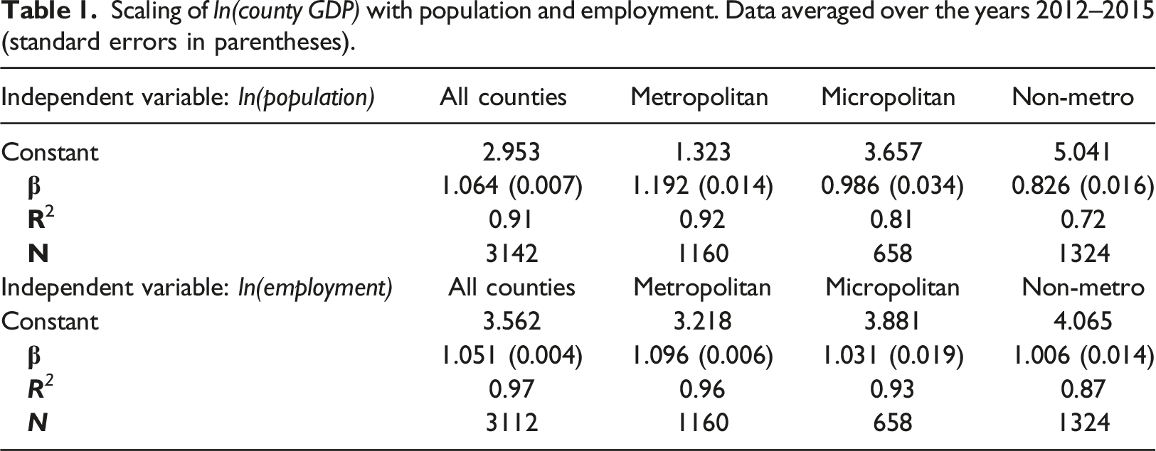
Scaling of ln(county GDP) with population and employment. Data averaged over the years 2012–2015 (standard errors in parentheses).

Independent variable: ln(population)	All counties	Metropolitan	Micropolitan	Non-metro
Constant	2.953	1.323	3.657	5.041
$β$	1.064 (0.007)	1.192 (0.014)	0.986 (0.034)	0.826 (0.016)
R²	0.91	0.92	0.81	0.72
N	3142	1160	658	1324
Independent variable: ln(employment)	All counties	Metropolitan	Micropolitan	Non-metro
Constant	3.562	3.218	3.881	4.065
β	1.051 (0.004)	1.096 (0.006)	1.031 (0.019)	1.006 (0.014)
R ²	0.97	0.96	0.93	0.87
N	3112	1160	658	1324

The BEA’s data on county-level GDP⁶ for the years 2012–2015 was matched with BEA data for county population and total employment.⁷ Table 2 shows the scaling coefficient for GDP against population and employment for the three types of counties classified by the BEA, as well as for all counties. The values for GDP, population, and employment have been averaged over the 4 four years to smooth fluctuations. For all counties, there is a slight superlinear effect (

β > 1

) associated with population size, but the scaling exhibited by “metropolitan counties”—defined using labor markets commuting flows—is as predicted by urban scaling theory (∼1.19), in fact the elasticity is slightly higher. For micropolitan counties, the increase in economic output is nearly linear with increases in population indicative that perhaps a population size threshold must be met before agglomeration effects kick-in. Interestingly, for non-urban counties, the increase in output scales with population akin to how networked infrastructure is predicted to do, sublinearly. This suggests that in non-urban counties, economic output is proportional to infrastructure, which in turn is suggestive of the absence of positive agglomeration effects. We note that identifying metropolitan counties by whether they are “core” or “outlying” does not alter the estimations in a meaningful way. Nor are the estimation results changed when spatial autocorrelation is controlled for.

Table 2.

Scaling of ln(county GDP) with ln(population) using the county classification schema of the Economic Research Service of the U.S. Department of Agriculture. Data averaged over the years 2012–2015 (standard errors in parentheses).

Metro		Constant	β	R²	N
1	in metropolitan areas of 1 million population or more	0.908	1.205 (0.018)	0.95	421
2	in metropolitan areas of 250,000 to 1 million population	1.411	1.182 (0.024)	0.94	434
3	in metropolitan areas of fewer than 250,000 population	1.748	1.161 (0.038)	0.89	346
Non-metro
4	urban population of 20,000 or more, adjacent to a metro area	4.919	0.872 (0.062)	0.58	212
5	urban population of 20,000 or more, not adjacent to a metro area	4.863	0.896 (0.073)	0.52	91
6	urban population of 2,500 to 19,999, adjacent to a metro area	4.357	0.898 (0.030)	0.61	586
7	urban population of 2,500 to 19,999, not adjacent to a metro area	4.997	0.851 (0.038)	0.54	425
8	rural or less than 2,500 urban population, adjacent to a metro area	5.443	0.753 (0.061)	0.56	220
9	rural or less than 2,500 urban population, not adjacent to a metro area	6.138	0.681 (0.033)	0.57	407

For metropolitan counties, superlinear scaling of output is lower with employment than population, mirroring the scaling of MSA level output with employment. For micropolitan and non-metropolitan counties, the scaling of output with employment is nearly linear, reflecting the role of the labor inputs in generating GDP. Table 2 shows the scaling relationships for county-level GDP against employment and population using the county classification schema by the Economic Research Service (ERS) of the US Department of Agriculture. The ERS’s rural–urban classification schema distinguishes metropolitan counties by population size and differentiates metropolitan and non-metropolitan counties by the degree of urbanization and adjacency to metropolitan areas. The scaling coefficients for GDP for the counties classified as metropolitan by the ERS are in line with is predictions by urban scaling theory.

The scaling results between county areal extent (measured in square miles) and residential population or employment indicate no relationship with slopes around 0.09 and R² of 0.05 for all years and types of counties. This result becomes less striking upon remembering that the boundaries of counties are the result of administrative fiat and historical contingency; county boundaries have little, if any, effect on the locational decisions of households or businesses. Moreover, as previously stated, the land area of counties enlarges when going from East to West.

The boundaries of Urbanized Areas deliberately ignore administrative considerations and attempt to encapsulate urban territory through contiguous and dense development, including residential and non-residential structures. Data on GDP is not reported for Urban Areas (nor is data on any other indicators of economic activity), but areal extent is reported.⁸ Table 3 shows the scaling coefficients of area against population for all Urban Areas and Urban Clusters of the U.S. for 2010, the most recent definition available (UAs and UCs are delineated during Population Census years). For urban areas—which capture urban life through population density (at least 386 persons per square kilometer) and built infrastructure—area scales with population as urban scaling theory predicts networked infrastructure should: β = 0.86, in agreement with theory (Bettencourt 2013). In the case of Urban Clusters, the scaling coefficient is nearly linear, so no density effects are apparent. Recall that urban clusters are urbanized areas with less than 50,000 inhabitants, so the linear scaling result suggests the presence of a size threshold before the benefits of shared network infrastructure come into play. Quantitatively, this result may be a consequence of population density inside urban clusters being similar to the threshold used to define them, so that the overall population density of urban clusters is a common number set by this threshold and area is proportional to population.

Table 3.

Scaling of area with population for Urbanized Areas (UAs) and Urban Clusters (UCs). Data for the year 2010 (both area and population are expressed in natural logarithm; standard errors in parentheses).

	UAs 2010	UCs 2010
Constant	−6.021	−6.892
$β$	0.861 (0.014)	0.948 (0.009)
R ²	0.89	0.81
N	497	3166

Discussion

In urban science, just as in physics or biology, definitions of meaningful units of analysis and measurement must follow from theory. Conversely, evaluating a theory presupposes observational units, and phenomenon are chosen to match what the theory prescribes must exist or occur. This empirical challenge has long been recognized in the study of cities since the richness of theoretical or modeling precepts are often not reflected in the definitions or data that scholars of cities have access to. Nevertheless, there is a common thread of agreement across economics, transportation studies, geography, and complex systems that functional cities are fundamentally networks of sustained socioeconomic interactions, and the delineation of urban space is emergent as a consequence of tradeoffs between net incomes derived from these exchanges and mobility costs, which vary with mode and technology.

The research reported here utilized new data for output (GDP) at different spatial scales to test the consequences of alternative definitions of functional cities to ascertain if the magnitude of agglomeration effects is consistent with predictions by Urban Scaling Theory. Urban scaling theory builds on over a century of urban models in geography, economics, and complex systems in advancing the central claim that urban areas result from self-consistently balancing incomes and costs thus defining functional urban areas implicitly through this budget constraint. There is no presumption in the classical models for urban agglomeration that just any concentration of humans, regardless of size, should exhibit the tell-signs of humans learning from, collaborating with, and coordinating among themselves, thereby increasing productivity and innovation. At the same time, agglomeration effects need not be spatially confined to metropolitan areas or even modern cities. The specific predictions made by urban scaling theory apply to spaces of intense social mixing and such spaces match some of the functional properties of cities, but the specific consequences of spatially embedded social mixing may or not be detectable in all spatial units for which data is collected. Measurable economic activity in U.S. counties, whose boundaries are the result of administrative and political path dependence, do reflect the presence of agglomeration economies (scaling effects), notwithstanding the arbitrariness.

A primary focus of the urban scaling has been the generative processes that underly the superlinearity associated with metropolitan areas. These generative processes obviously must exist in the spatial subcomponents of cities, as we show here. What may be surprising is how spatially concentrated the activities are in the urbanized components of metropolitan areas. The high scaling coefficients of particularly large metropolitan areas may be the result of more uniform urbanization across the entirety of the metropolitan area, which is not typical of smaller units. This unpacking of the interaction structure of cities over populations, space, and time is a very fertile ground for future studies, as data continues to improve in precision and scope.

Similar investigations are possible in other nations as well and should be the focus of a parallel investigation to the work described here. For example, in European Union nations, there are data reported for GDP at the NUTS3 level (similar to counties, but somewhat variable between nations) and at the metropolitan area level (Bettencourt and Lobo, 2016). In China, there are data for districts and counties and for Prefectural level cities (Zuend and Bettencourt, 2019), a similar situation to Japan where metropolitan definitions are also more advanced. Urban agglomerations in India display some of the scaling properties of metropolitan areas, results which should be examined at a finer grained resolution (Sahasranaman and Bettencourt, 2019). More challenging, but arguably even more important, is the development of a rich empirical basis and analyses of fast growing, developing urban areas, especially in Africa and Asia, where networks of economic activity, civic institutions, and infrastructure are still forming, opening up rich windows into the nature of dynamical processes whereby large urban areas come together and develop.

Footnotes

Acknowledgments

We would like to thank the reviewers for their thoughtful comments and efforts towards improving our manuscript.

Author contributions

D.S., L.M.A.B., and J.L. designed research; D.S., L.M.A.B., and J.L. performed research; and D.S. and J.L. wrote the article.

Declaration of conflicting interests

The author(s) declared no potential conflicts of interest with respect to the research, authorship, and/or publication of this article.

Funding

The author(s) received no financial support for the research, authorship, and/or publication of this article.

Ethical approval

No human subjects were involved in the research reported here.

Notes

Author biographies

Deborah Strumsky, trained as a Regional Scientists, is a Faculty at the Centre for Entrepreneurship and Spatial Economics, Jönköping International Business School, Jönköping University (Sweden). Her primary research focus in on invention and technological change with a special interest in the creation of technological novelty in urban areas.

Luis Bettencourt is a Professor of Ecology and Evolution and Associate Faculty in Sociology, and the Inaugural Director of the Mansueto Institute for Urban Innovation at the University of Chicago (USA). His research investigates fundamental processes of biological and social organization and evolution in complex systems, with an emphasis on urban environments.

José Lobo a faculty at the School of Sustainability, College of Global Futures, Arizona State Univerisyt (USA) is an urban economist interested in the fundamantal social processes underpinning cities and urbanization.

References

Alonso

(1964) Location and Land Use. Cambridge (MA): Harvard University Press.

Angel

(2012) Planet of Cities. Cambridge, MA: Lincoln Institute of Land Policy.

Barabasi

(2016) Network Science. Cambridge: Cambridge University Press.

Bartheley

(2017) The Structure and Dynamics of Cities: Urban Data Analysis and Theoretical Modeling. Cambridge: Cambridge University Press.

Batty

(2013) The New Science of Cities. Cambridge (MA): The MIT Press.

Batty

Ferguson

(2011) Defining city size. Environment and Planning B: Planning and Design 38: 753–756.

Berry

BJL

(1967) Generalization of the Metropolitan Area concept. Proceedings of the Social Statistics Section of the American Statistical Association: 86–91.

Berry

BJL

Goheen

Goldstein

(1969) Metropolitan Area Definition; a Re-evaluation of Concept and Statistical Practice. Washington, D.C.: United States Bureau of the Census.

Bertaud

(2018) Order without Design: How Markets Shape Cities. Canbridge (MA): The MIT Press.

10.

Bettencourt

LMA

(2013) The origins of scaling in cities. Science 340: 1438–1441.

11.

Bettencourt

LMA

(2014) Impact of changing technology on the evolution of complex informational networks. Proceedings of the IEEE 102: 1878–1891.

12.

Bettencourt

LMA

Lobo

(2016) Urban scaling in Europe. Journal of the Royal Society Interface 13: 20160005.

13.

Bloom

Canning

Fink

(2008) Urbanization and the wealth of nations. Science 319: 772–775.

14.

Bretagnolle

Pumain

Vacchiani-Marcuzzo

(2009) The organisation of urban systems. In: Lane

Pumain

Van der Leeuw

, et al. (eds), Complexity Perspectives in Innovation and Social Change. New York: Springer, pp. 197–220.

15.

Bretagnolle

Delisle

Mathian

, et al. (2015) Urbanization of the United States over two centuries: an approach based on a long-term database (1790-2010). International Journal of Geographical Information Science 29: 850–857.

16.

Brueckner

(2011) Lectures in Urban Economics. Cambridge (MA): The MIT Press.

17.

Bureau of Economic Analysis (2015) Measuring the Economy: A Primer on GDP and the National Income and Product Accounts. Washington, D.C.: U.S. Department of Commerce. https://www.bea.gov/sites/default/files/methodologies/nipa_primer.pdf

18.

Carneiro

(2000) The transition from quantity to quality: A neglected causal mechanism in accounting for social evolution. Proceedings of the National Acadey of Sciences of the USA 97: 12926–12931.

19.

Cesaretti

Lobo

Bettencourt

LMA

, et al. (2016) Population-Area Relationship for Medieval European Cities. Plos One. 11: e0162678. DOI: 10.1371/journal.pone.0162678.

20.

Colby

(1933) Centrifugal and centripetal forces in urban geography. Annals of the Association of American Geographers 23: 1–20.

21.

Cromartie

(2019) Rural Classifications. Economic Research ServiceU.S. Department of Agriculture. https://www.ers.usda.gov/topics/rural-economy-population/rural-classifications/

22.

Duranton

Puga

(2004) Micro-foundations of urban agglomeration economies. In: Henderson

Thisse

J-F

(eds), Handbook of regional and urban economics 2063–2117. Amsterdam, The Netherlands: Elsevier.

23.

Easley

Kleinberg

(2010) Networks, Crowds, and Markets: Reasoning about a Highly Connected World. New York: Cambridge University Press.

24.

Federal Register (2011) Urban Area Criteria for the 2010 Census: Notice. Washington, D.C.: U.S. Census Bureau, Department of Commerce, 76. No. 164.

25.

Fox

(1968) Functional economic areas and consolidated urban regions of the United States. Statistical Reporter 68: 145–148.

26.

Fox

Kumar

(1965) The functional economic area: Delineation and implications for economic analysis and policy. Papers of the Regional Science Association 15: 57–85.

27.

Fujita

Krugman

Venables

(1999) The Spatial Economy: Cities, Regions, and International Trade. Cambridge (MA): The MIT Press.

28.

Gehlke

Biehl

(1934) Certain Effects of Grouping Upon the Size of the Correlation Coefficient in Census Tract Material. Journal of the American Statistical Association. Online ahead of print.

29.

Glaeser

(2011) Triumph of the City: How Our Greatest Invention Makes Us Richer, Smarter, Greener, Healthier, and Happier. New York: Penguin Press.

30.

Glaeser

Sacerdote

Scheinkman

(2003) The social multiplier. Journal of the European Economic Association, 1: 345–353.

31.

Golob

Beckmann

Zahavi

(1981) A utility-theory demand model incorporating travel budgets. Transportation Research Part B: Methodological 15: 375–389.

32.

Gomez-leviano

Youn

Bettencourt

LMA

(2012) The Statistics of Urban Scaling and Their Connection to Zipf’s Law. Plos One. DOI: 10.1371/journal.pone.0040393.

33.

Granovetter

(1973) The strength of weak ties. American Journal of Sociology 78: 1360–1380.

34.

Guci

Mead

Panek

(2016) A Research Agenda For Measuring GDP at the County Level. Washington, D.C.: Bureau of Economic AnalysisU.S. Departmen of Commerce. https://www.bea.gov/index.php/system/files/papers/WP2016-4.pdf

35.

Hayward

(1846) The New England Gazetteer. Boston: John Hayward.

36.

Henderson

(1988) Urban Development: Theory, Fact and Illusion. New York: Oxford University Press.

37.

Isard

(1956) Location and Space-Economy: A General Theory Relating to Industrial Location, Market Areas, Land Use, and Urban Structure. Cambridge (MA): The MIT Press.

38.

Jackson

(2008) Social and Economic Networks. Princeton: Princeton University Press.

39.

Jiao

Zhao

Liu

Wang

(2020) Assessment of urban land use efficiency in China: A perspective of scaling law. Habitat International 99. https://doi.org/10.1016/j.habitatint.2020.102172

40.

Johnson

Earle

(2000) The Evolution of Human Societies: From Foraging Group to Agrarian State. Stanford: Stanford University Press.

41.

Jones

Romer

(2010) The New Kaldor Facts: Ideas, Institutions, Population, and Human Capital. AMERICAN ECONOMIC JOURNAL: MACROECONOMICS 2(1): 224–245.

42.

Katz

(2006) Indicators for complex innovation systems. Research Policy 35: 893–909.

43.

Kostof

(1991) The City Shaped: Urban Patterns and Meanings through History. Boston, MA: Bullfinch.

44.

Krugman

(1991) Increasing returns and economic geography. Journal of Political Economy 99: 483–499.

45.

Lobo

Bettencourt

LMA

Smith

, et al. (2020) Settlement scaling theory: Bridging the study of ancient and contemporary urban systems. Urban Studies 57: 731–747.

46.

Louf

Barthelemy

(2014) A typology of street patterns. Journal of the Royal Society Interface 11(101): 1–7.

47.

Marchetti

(1994) Anthropological invariants in travel behavior. Technological Forecasting and Social Change 47: 75–88.

48.

Meier

(1962) A Communications Theory of Urban Growth. Cambridge (MA): The MIT Press.

49.

National Association of County Governments (2013) History of County Governments. https://web.archive.org/web/20130411042056/http://www.naco.org/Counties/Pages/HistoryofCountyGovernmentPartI.aspx

50.

Nordbeck

(1971) Urban allometric growth. Geografiska Annaler. Series B, Human Geography 53: 54–67.

51.

Openshaw

(1983) The Modifiable Areal Unit Problem. Norwick: Geo Books.

52.

Ortman

Cabaniss

AHF

Sturm

, et al. (2015) Settlement scaling and increasing returns in an ancient society. Science Advances 1: e1400066.

53.

O’Sullivan

(2011) Urban Economics. New York: McGraw-Hill.

54.

Pumain

(2000) Settlement systems in the evolution. Geografiska Annaler. Series B, Human Geography 82: 73–87.

55.

Ratcliffe

(2015) A Century of Delineating a Changing Landscape: The Census Bureau’s Urban and Rural Classification, 1910 to 2010. Washington, D.C.: Geography Division, U.S. Census BureauU.S. Department of Commerce. https://www2.census.gov/geo/pdfs/reference/ua/Century_of_Defining_Urban.pdf

56.

Ratcliffe

Burd

Holder

, et al. (2016) Defining Rural at the U.S. Census Bureau. In ACSGEO-1. Washington, D.C.: Geography Division, U.S. Census BureauU.S. Department of Commerce. https://www2.census.gov/geo/pdfs/reference/ua/Defining_Rural.pdf

57.

Rosenthal

Strange

(2001) The determinants of agglomeration. Journal of Urban Economics 50: 377–393.

58.

Sahasranaman

Bettencourt

LMA

(2019) Urban geography and scaling of contemporary Indian cities. Journal of the Royal Society Interface 16. DOI: 10.1098/rsif.2018.0758.

59.

Segal

(1976) Are there Returns to Scale in City Size? Review of Economics and Statistics 58: 339–350.

60.

Sennett

(1977) The Fall of Public Man. New York: Knopf.

61.

Smith

(2019) Energized crowding and the generative role of settlement aggregation and urbanization. In: Gyucha

(ed), Coming Together: Comparative Approaches to Population Aggregation and Early Urbanization. Albany, NY: State University of New York Press, pp. 37–58.

62.

Southall

(1998) The City in Time and Space. Cambridge: Cambridge University Press.

63.

Speare

William

(1991) Metropolitan Areas of the Future: Issues and Definitions. Proceedings of the Government Statistics Section of the American Statistical Association.

64.

Storper

(2013) Keys to the City: How Economics, Institutions, Social Interaction, and Politics Shape Development. Princeton: Princeton University Press.

65.

Strange

(2008) Strange W.C. (2008) Urban Agglomeration. In: Durlauf

Blume

(eds), The New Palgrave Dictionary of Economics. London: Palgrave Macmillan.

66.

Strumsky

Lobo

Mellander

(2019) As different as night and day: Scaling analysis of Swedish urban areas and regional labor markets. Environment and Planning B: Urban Analytics and City Science. DOI: 10.1177/2399808319861974.

67.

Sveikauskas

(1975) The Productivity of Cities. Quarterly Journal of Economics 89: 393–413.

68.

Truesdell

(1949) The Development of the Urban-Rural Classification in the United States: 1874-1949. U.S. Department of Commerce, Current Population Reports, Series P-23, No. 1.

69.

United States Census Bureau (1994) Geographic Areas Reference Manual. Washington, DC: Geography DivisionU.S. Department of Commerce.

70.

Uslaner

(1976) The pitfalls of per capita. American Journal of Political Science 20: 125–133.

71.

von Thünen

(1966) The Isolated State. Oxford: Pergamon Press.

72.

Wilson

(2020) Metropolis: A History of the City, Humankind's Greatest Invention. New York: Doubleday.

73.

Wirth

(1938) Urbanism as a way of life. American Journal of Sociology 44: 1–24.

74.

Wong

DWS

(2009) The modifiable areal unit problem (MAUP). In: Fotheringham

Rogerson

(eds), The SAGE handbook of spatial analysis. Los Angeles: Sage, pp. 105–124.

75.

Zahavi

(1974) Traveltime Budgets and Mobility in Urban Areas. Federal Highway Administration Report FHWA PL-8183. Washington, D.C.: U.S. Department of Transportation.

76.

Zünd

Bettencourt

LMA

(2019) Growth and development in prefecture-level cities in China. Pls One 14(9). https://doi.org/10.1371/journal.pone.0221017