
Abstract
Comparing transit operations and performance over time is often challenging due to changes in route identifiers and service patterns. It is particularly difficult if the analysis period spans a major network design change where bus routes are realigned and renamed. This paper presents a new open-source software package that simplifies longitudinal transit performance analysis by decomposing a bus network into block-length segments that remain stable over time. The package then matches transit networks across time periods using segment geometry rather than potentially unstable route or stop identifiers. This package provides an efficient method for transit planners, advocacy groups, policy makers and urban scientists to analyze changes in transit performance over time without any prior knowledge of network design changes.
Introduction
Transit planners, analysts and external stakeholders often seek to understand how the supply and quality of bus transit service changes over time. In most applications, the supply and quality of service is quantified through performance metrics such as reliability and crowding, which are measured and reported at the route or stop level and tabulated by route or stop identifiers (Kittelson and Associates 2003). Bus networks are not stable over time, however; the patterns of stops that constitute a bus route are revised periodically and arbitrary stop numbers are reassigned to entirely different locations (Weckström et al., 2021). Such changes make it difficult to conduct a comprehensive performance comparison based only on route or stop identifiers (Weckström et al., 2019). In order to review the performance of a redesigned network, an analyst would need to have knowledge of each service change. Extending the analysis to include the entire network across many years or decades would require a tremendous amount of manual effort and the results would be difficult to validate.
A systematic method of comparing bus service and performance that is based on stable reference geographies, rather than identification numbers, can be used for consistent representation over time. However, shifting toward a geographic representation for the transit network presents challenges in terms of scope and interpretation. If the city block is taken as the unit of measurement, there would be more than ten thousand data points for large transit networks. Spatial visualization can mitigate these issues, however, by representing large sets of disaggregate transit data in a familiar setting (Batty 2007). Visualization allows for identification of spatial trends, such as neighborhoods with declining quality of service, and provides additional geographic context that is difficult to elicit from a tabular representation.
In this paper, a new map matching-based method is proposed for decomposing a bus transit network into city block-length segments using a standardized machine-readable transit schedule and open road network data. These segments are identified based on geography rather than route or stop numbers, allowing them to be compared over long periods of time. Then, performance metrics are assigned to each geographic measurement unit and aggregated to enable long-term comparison of service quality along each block.
Prior studies have established methods for matching a transit schedule represented in the General Transit Feed Specification (GTFS) format to a representation of the road network, although not for longitudinal comparison (Li 2012; Dimond et al., 2016; Ordóñez Medina 2016; Wessel et al., 2017; Bhagat-Conway 2018). The concept of splitting routes at road intersections and stops was inspired by a similar project intended for aggregating transit performance within shared segments (Brown 2021). None of these studies proposes a geographically based representation system for public transit that can be used for longitudinal comparison.
There are surprisingly limited comprehensive efforts to analyze the temporal evolution of bus transit service. The studies that have reviewed the performance of individual bus routes or entire networks before and after service changes tend to focus on highly aggregate measures such as changes in accessibility or total travel time (Wu and Hine 2003; Grengs 2004; El-Geneidy and Levinson 2007; Kim et al., 2018; Bertolaccini 2018; Handley et al., 2019). Another study reviews the travel time changes that arise from a large scale network redesign of the bus network in Helsinki, Finland (Weckström et al., 2019). The authors note that one issue in comparing schedules before and after the network changes is the differing stop identifiers, which must be manually corrected.
To the authors’ knowledge, this is the first effort to develop a widely generalizable method for evaluating temporal changes in transit performance measured at a disaggregate level. The open-source code package used to implement the methods described herein is available at https://github.com/jtl-transit/busdecomp. Two empirical case studies are included in the supplemental materials to demonstrate the strength of these methods relative to identifier-based comparisons in real transit planning and policy analysis applications.
Description of the software package
A flowchart representing the overall process is presented in Figure 1, and each subprocess is described in detail below. Flowchart representing the process for decomposing and comparing a bus network over time.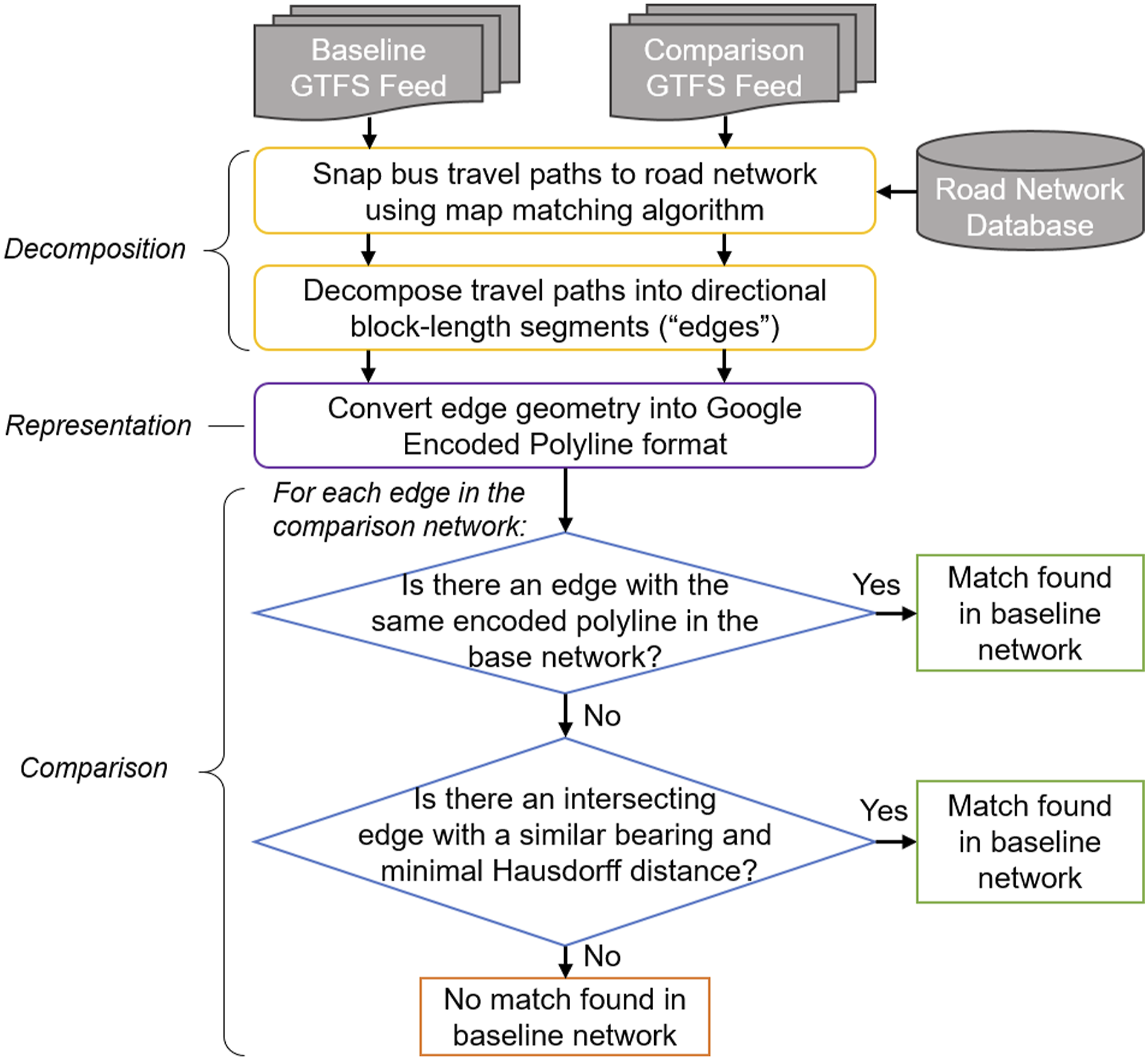
Block-level decomposition
An appropriate unit of analysis must be chosen to enable consistent representation of a bus transit network over time. The goal is to select the largest possible unit such that aggregate transit service is consistent across the entire length. The distance between two intersections is therefore used, with additional boundaries at mid-block bus stops. This unit of analysis, which will now be referred to as an “edge,” is a stable geographic unit across which bus service and performance can be measured.
The decomposition method uses a machine-readable transit schedule that includes information related to the transit network geometry and schedules. The standard GTFS feed contains the stop_times.txt table, from which the unique stop sequences (or “patterns”) that constitute a bus trip can be extracted. The latitude and longitude coordinates of each stop are collected from the GTFS stops.txt table. Patterns are then converted to a sequence of coordinates that represent the path of the bus. These sequences of coordinates are used as inputs for a map matching process, which snaps the path of the bus to the road network. The optional shapes.txt file in a GTFS feed can be used if available to improve map matching accuracy by adding coordinates between bus stops. The code package linked in this paper uses the open-source Valhalla map matching library (Valhalla 2020).
The minimum inputs required for map matching are the coordinates of each bus stop and a standard representation the road network. Multi-lane streets must be represented as a single edge in the road network. Road network files can be downloaded from OpenStreetMap (OSM) (OpenStreetMap contributors 2020), an open data source. The map matching service builds a graph representation of the road network from the OSM input data, where the nodes of the graph represent intersections and the edges of the graph represent the street between two intersections. The graph is directed, meaning that there is a separate edge for each direction of travel on a two-way street.
Given a pair of input coordinates for routing, the map matching algorithm identifies the nearest edges within the road network, then computes the shortest path between the input coordinates. Li (2012) shows that a shortest-path map matching algorithm is accurate for 98% of transit segments. The output includes the set of edges traversed by the shortest path between the input coordinates. The output also includes a sequence of coordinates that creates a line segment representation of the shortest path.
These output coordinates are then converted into polylines. An additional step is required to generate block-level edges. First, the polylines are split at street intersections to create directional edges that are approximately equivalent to a city block. Then the lines are split at mid-block bus stops, which allows differentiation of performance metrics like crowding and passenger load before and after a stop event. A distance threshold can be used for determining which stops are considered to be mid-block. The threshold improves visualization by avoiding the creation of small edges between bus stops and nearby intersections. An illustration of the edge decomposition is shown in Figure 2, where a bi-directional bus route is split into 14 edges. The diagram on the right demonstrates the output when a 75 foot intersection distance is applied. Example of bus network discretization into geographic edges, with and without an intersection distance threshold applied.
The geometry of each edge is stored as a sequence of coordinates. The geometry can be straight or curved depending on the underlying road network geography, allowing the method to be applied in cities with irregular or winding roads; the average edge in the Massachusetts Bay Transportation Authority (MBTA) bus network in the Boston, Massachusetts area is represented by more than seven coordinate pairs. For each period, the stop pairs corresponding to each edge are stored to allow route or stop-level performance metrics to be assigned to the edges. In the case that multiple routes serve a single edge, the performance metrics are aggregated across routes to generate an edge-average or edge-sum measure. Certain passenger and infrastructure-based metrics such as passenger flow and travel speed could also be aggregated directly across routes serving the same edge because edges are defined such that transit service is consistent across the entire edge.
Geographic representation
The edges generated in the previous step are more stable than route or stop IDs over time and are therefore used as the basis for longitudinal comparison. The edges are initially stored as the set of coordinates representing the geography of the edge. The comparison between edges could be conducted directly by checking geometric equivalence, but such operations are typically too computationally intensive to be used at the network scale. To enable a more efficient method of comparison, the edge geometries are encoded as a text string using the Google Encoded Polyline compression algorithm (Google Developers 2021). Text encoding improves the computation time for comparison between two time periods by two orders of magnitude. The algorithm implements rounding after the fifth decimal place of the latitude and longitude decimal degrees, which produces a maximum error of approximately 0.5 m. The compression loss is inconsequential for this application given that the edges are typically dozens of meters in length.
Longitudinal comparison
To match edges across two time periods, the first step is to screen for exact matches between the encoded text strings described in the previous section. The rate of matching depends on the number of changes to the bus network between the two comparison periods. An edge match indicates that a block with bus transit service in the earlier period is also served in the later period. If an edge from the earlier period does not have a match, that indicates that the edge is no longer served in the later period. If an edge from the later period does not have a match, then a new service has been launched along the edge that did not exist during the first period.
If the comparison is conducted for the same service area across two time periods, the vast majority of edges in both periods would be expected to have a match. For example, a comparison of the MBTA bus network found that 84% of the 42,796 edges in the January 2011 network were also included in the January 2021 network. The remaining 16% (7,129 edges) were no longer being served, but an additional 5,162 new edges were included in the January 2021 network.
In some cases, the encoded polylines of two segments may not match exactly, but the segments could be considered equivalent for the purpose of this analysis. One example is a segment that begins at a bus depot with multiple bays, where the bays are distinct stops with distinct coordinates in GTFS. Another scenario where this issue could arise is when an agency revises the coordinates of a bus stop in GTFS between successive feeds for greater accuracy. A third scenario can occur when multiple agencies serve the same physical bus stop and they report slightly different coordinates for the same bus stop. In each of these scenarios, the encoded polylines may not match, yet the edges should be matched for comparison. Simple methods such as matching stops using buffers can create errors by creating false matches between nearby (but not identical bus stops), therefore a more accurate method is used.
First, assume there are two periods with different service patterns, Periods A and B. When comparing edges from Period A to Period B, any edges from Period A that are not matched during the first screening are stored in a list. Then, spatial intersections between the unmatched Period A edges and the full set of Period B edges are identified. The complexity of the intersection operation is linear with respect to the number of edges in the network; checking for intersection between one edge and full set of edges in the January 2021 MBTA network takes less than 0.2 s using the Shapely package for Python 3.9. The Hausdorff distance between the intersecting edges is computed and must be below a maximum threshold for matching. Finally, to confirm a match based on the intersection of two segments, it is necessary to check that the edges have the same bearing, as one segment could intersect another segment traveling in the opposite direction. The bearing is approximated by the angle of a vector between the first and last coordinates of the segment. If the two angles are within a certain tolerance, the segments are considered a match. Comparing trajectories based on Hausdorff distance and bearing is a common approach used in map matching literature (Hashemi and Karimi 2016; Jiang et al., 2022).
There is a final consideration specific to longitudinal comparison. Over time, new bus stops may be introduced and old ones may be removed. This has the effect of creating two different edges along the same block for the two comparison periods. To avoid this scenario, the individual edges for each network should be created by splitting at any mid-block bus stop that exists in either bus network.
Due to the geographic decomposition method and the encoded polyline representation, comparing a bus transit network across two time periods is computationally efficient, taking 2 min on a dual-core Intel i7-6600U CPU with 16 GB of RAM.
Discussion
The software package presented in this paper lowers the barrier to conducting comprehensive reviews of service changes over the course of several years. Any changes to route or stop IDs across the study period are automatically incorporated into the results. This approach also retains the original geographic structure of the network, unlike graph-based representations of public transit network changes (e.g. Feng et al., 2019). This software package can be used for comparative policy analysis without any a priori knowledge of the bus networks or service changes. It could be adopted by agency staff and external stakeholders to compare local service quality against other peer agencies and to create helpful visualizations for communication with the public.
There are limitations to this method. First, the software package uses a static GTFS feed as the source of network and timetable data, but many transit agencies do not maintain GTFS feeds. However, the decomposition method could easily be adapted for compatibility with other similar machine-readable transit data standards. Second, if no additional information is available, the map matching process assumes that the shortest path between two stops is followed. In most cases this assumption is valid, but it may not hold for all paths, especially when stops are spaced farther apart (Li 2012; Ordóñez Medina 2016). These methods also assume a road network that is stable over time, which may not be true, especially in rapidly developing regions. Lastly, OSM is proposed as the source of road network information to ensure that the method remains open source and generalizable. Research has found OSM to be reasonably accurate (Brovelli et al., 2016), but it is populated and maintained by volunteer contributors, so its accuracy cannot be guaranteed.
The methods described in this paper can be used to facilitate many new research projects that would otherwise require a prohibitive level of effort. Future applications of this research include studying the growth of bus transit networks over time. Transit network data could be combined with socioeconomic indicators to examine how service changes have affected different groups. Statistical analysis of the bus network growth patterns combined with ridership data across different urban areas could also be used to identify causal relationships between network evolution and ridership.
Supplemental Material
Supplemental Material - An open-source program for spatial decomposition of bus transit networks
Supplemental Material for An open-source program for spatial decomposition of bus transit networks by Nicholas S Caros, Anson F Stewart and John Attanucci in Environment and Planning B: Urban Analytics and City Science.
Footnotes
Acknowledgements
The authors would like to thank Alissa Zimmer and Anna Gartsman of the Massachusetts Bay Transportation Authority (MBTA) for encouraging this research and providing early feedback. The authors would also like to thank the MBTA and the Chicago Transit Authority for their generous funding of this research project.
Declaration of Conflicting Interests
The author(s) declared no potential conflicts of interest with respect to the research, authorship, and/or publication of this article.
Funding
The author(s) disclosed receipt of the following financial support for the research, authorship, and/or publication of this article: This work was supported by the Chicago Transit Authority and Massachusetts Bay Transportation Authority.
Supplemental Material
Supplemental material for this article is available online.
References
Supplementary Material
Please find the following supplemental material available below.
For Open Access articles published under a Creative Commons License, all supplemental material carries the same license as the article it is associated with.
For non-Open Access articles published, all supplemental material carries a non-exclusive license, and permission requests for re-use of supplemental material or any part of supplemental material shall be sent directly to the copyright owner as specified in the copyright notice associated with the article.