
Abstract
Racial residential segregation is a longstanding topic of focus across the disciplines of urban social science. Classically, segregation indices are calculated based on areal groupings (e.g., counties or census tracts), with more recent research exploring ways that spatial relationships can enter the equation. Spatial segregation measures embody the notion that proximity to one’s neighbors is a better specification of residential segregation than simply who resides together inside the same arbitrarily drawn polygon. Thus, they expand the notion of “who is nearby” to include those who are geographically close to each polygon rather than a binary inside/outside distinction. Yet spatial segregation indices often resort to crude measurements of proximity, such as the Euclidean distance between observations, given the complexity and data requirements of calculating more theoretically appropriate measures, such as distance along the pedestrian travel network. In this paper, we examine the ramifications of such decisions. For each metropolitan region in the U.S., we compute both Euclidean and network-based spatial segregation indices. We use a novel inferential framework to examine the statistical significance of the difference between the two measures and following, we use features of the network topology (e.g., connectivity, circuity, throughput) to explain this difference using a series of regression models. We show that there is often a large difference between segregation indices when measured by these two strategies (which is frequently significant). Further, we explain which topology measures reduce the observed gap and discuss implications for urban planning and design paradigms.
Introduction
An exceedingly common abstraction in applied spatial analysis is the use of Euclidean distance as a proxy measure for geographic proximity (which is, itself, often a proxy for the frequency of social interaction). It is the geographical scientist’s equivalent to the physicist’s spherical cow, 1 or the economist’s perfect market: a useful abstraction that helps partially explain a much more complex underlying process, however imperfectly. A major difference in spatial analysis, however, is that scientists from many disciplines often fail to realize how simplified the assumption of Euclidean distance is when traversing the built or natural environment. While, in general, simple proximity is a reasonable heuristic for understanding Tobler’s Law (Tobler, 1970), the behavioral realities of movement and social interaction in complex urban environments often require a more thoughtful model.
More directly, cities, regions, and neighborhoods are not featureless planes in which agents have perfect freedom of mobility. Rather, they are multifaceted environments populated by highways, canyons, rivers, mountains, railroad tracks, alleyways, and power plants. To facilitate movement in this environment, an interleaved transportation system provides passageways through discrete locations, and conditions how easy it is to move throughout the region and interact with individuals in other parts of the region. Although pure Euclidean distance can proxy this system, the urban design decisions that govern how and where networks are located, as well as the natural features like elevation or water features play an important, albeit underexamined, role in mediating social interactions.
One particular topic where a full understanding of space would provide significant benefits is segregation analysis, a longstanding topic of focus across the disciplines of urban social science. Classically, segregation indices are calculated based on areal groupings (e.g., counties or census tracts), with more recent research exploring ways that spatial relationships can enter the equation. Spatial segregation measures embody the notion that proximity to one’s neighbors is a better specification of residential segregation than simply who resides together inside the same arbitrarily drawn polygon. Thus, they expand the notion of “who is nearby” to include those who are geographically close to each polygon rather than a binary inside/outside distinction. Yet spatial segregation measures often resort to crude measurements of proximity, such as the Euclidean distance between observations, given the complexity and data requirements of calculating more theoretically appropriate measures, such as distance along the pedestrian travel network.
In this paper, we examine the relationship between pedestrian network characteristics and the measurement of metropolitan segregation. In doing so, we examine three research questions in turn: first, how much does the operationalization of space matter for segregation measurement? More specifically, how large is the difference between Euclidean-based and network-based measures of spatial segregation? Second, if differences exist between Euclidean and network measures, are they large enough that they cannot be attributed to chance? Third, what characteristics of the travel network are related to the observed difference in measurement? If there is a large and/or systematic difference between traditional spatial measurements and those leveraging more realistic measurements of distance, then there may be much to learn about the contribution of network structure and design when seeking to maximize urban integration.
Urban infrastructure and social interactions
Since the inception of city planning, the relationship between social interactions and the built environment has been a topic of intense focus for both social scientists and urban designers (Talen, 2017). The normative concepts of urban utopias prescribed by architects like Ebeneezer Howard, Frank Lloyd Wright, and Le Corbusier included distinct visions for how densely populated and separated/integrated land uses could facilitate the ideal level of interaction between a resident and (a) her neighbors, and (b) her natural surroundings (Campbell and Fainstein, 1996; Corbusier, 1986; Howard and Osborn, 2001). Combining these visions with ideas from Wirth (1938) and the famous “neighborhood unit plan” articulated by Perry (1929), large-scale developers like James Rouse developed concepts for New Towns like Columbia, Maryland that were based largely on the design of insular street networks (Olsen, 2003).
At their best, these designs were intended to foster community for the residents that live within them, and ensure that amenities like school, shopping, employment, and leisure are all within a walkable distance from the neighborhood’s core. From a more cynical perspective, the cul-de-sac patterns and interspersed greenways of the ‘neighborhood unit plan’ helped codify the American ideal of white flight and the picturesque upper-middle class neighborhood, using both urban design and land-use policy as informal mechanisms of residential sorting. Thus, although the arrangement of people in space has been a focus of urban thought for more than a century, it remains an open question how well features of the real urban fabric are represented in quantitative models of social interaction, such as segregation indices—and whether urban design characteristics shape our perception of these patterns.
Now we have both the tools and the logic to test these assumptions and understand the role of abstractions such as Euclidean distance-based measures in our assessment of critical social processes such as residential segregation. Fast graph algorithms allow us to construct more realistic concepts of spatial weights matrices, and computational statistics allow us to construct and test realistic null hypotheses about the allocation of urban population groups. Here, we examine the role of street network topology in the appropriate measurement of urban segregation. Our goals are twofold.
First, we aim to understand the implications of simple Euclidean distance-based abstractions when conducting formal spatial analyses; that is, do we find substantive differences in results when more realistic concepts of spatial relationships (e.g., network connectivity) are considered? Second, we aim to explore the elements of urban design (particularly the street network configuration) in widening the gap between analytical abstraction and empirical reality. More simply, we aim to understand whether certain elements of the street network are associated with a greater difference in measured segregation. With this knowledge, urban designers and planners can begin with more inclusive communities from the beginning.
Measuring segregation in space
Incorporating distance into segregation indices
In a foundational contribution, White (1983) conceives of segregation in terms of spatial interaction and formulates a spatial dissimilarity index using an exponential decay function to weight the proximity between observed census units. Despite the importance of the contribution, the application of White’s technique has never become widespread, perhaps in part because of the difficulty in operationalizing the index prior to modern GIS. Through the 1990s, a surge of research on spatial segregation indices examined different methods for incorporating space, leveraging the growing GIS capacity of the era. An important critique of the time is given by Wong (1993) who shows that spatial segregation indices based on contiguity between adjacent units provide poor definitions of the local neighborhood. This criticism is based in part because geographic units are heterogenously sized and also because polygon adjacency may be a poor measurement of “nearness.” Additional work has explored the sensitivity of segregation measures to the modifiable areal unit problem (MAUP) (Openshaw, 1984), and by extension, the importance of spatial scale (Wong, 1997, 2004). Some authors have also developed spatial extensions or decompositions of popular indices such as the Gini index (Dawkins, 2004; Rey and Folch, 2011).
In a canonical contribution to the segregation literature, Reardon and O’Sullivan (2004) develop a generalized framework for creating spatial segregation indices using a generic formulation of the neighborhood. They also show that the spatial information theory index
A variety of authors have also begun to examine the role of spatial scale. In an important advance in segregation methods, Reardon et al. (2008) develop a method for understanding the implications of multiscalar segregation by varying the distance parameter used to compute the local environment in a spatial segregation index. Following, Reardon et al. (2009) and Lee et al. (2008) apply the framework to a large set of metropolitan regions in the U.S., demonstrating a wide variety of macro versus micro-scaled patterns, and other work has explored the role of multiscalar change over time (Bailey, 2012; Fowler, 2016). Another prominent body of work builds on this work, exploring the notion of “egohoods,” where each household has its own concept of the neighborhood that extends outward and partially overlaps with others nearby (Hipp and Boessen, 2013; Petrović et al., 2018, 2019). Even more recently, additional measurement techniques have been developed that help summarize multiscalar patterns using a single index (as opposed to an array or a ratio) (Bézenac et al., 2022; Clark et al., 2015; Olteanu et al., 2019; Östh et al., 2015). This research has provided clear evidence not only of the importance of considering spatial relationships in segregation measurement, but also the ways that misspecification of space (such as application of an inappropriate scale) can lead to a skewed concept of the phenomenon under study.
Transportation and social interaction
Elsewhere, scholars have examined the role of physical barriers and built features of the urban environment in facilitating social contact. For example, Grannis (2005) shows social interactions are more frequent inside “T-communities” defined by street networks (Grannis, 2005), and Roberto (2018) uses street networks to measure segregation in a small-scale case study, and shows that segregation in Pittsburgh is higher when measured according to network distance. These contributions emphasize a long-recognized but understudied element of metropolitan segregation patterns, namely, that transport networks, physical barriers, and other factors such as elevation or congestion condition the expected potential for social interaction in space. For example, work in sociology has shown the importance of street network connectivity in fostering social networks inside small urban geographic zones (Grannis, 1998). The natural logic underlying these findings is that street networks can help insulate urban environments and provide greater exposure to residents living inside “the neighborhood” than those who live outside, but this distinction can be masked easily when measuring metropolitan space using Euclidean distances.
A depiction of the difference between network travel distance and “as the crow flies” distance is shown in Figure 1. The figure shows an origin marked with an X in the center and two different polygons representing a one-mile travel distance using different methods in the cities of San Clemente and Chicago. The small polygon depicts the total extent accessible from the origin point when traveling along the pedestrian network, whereas the larger polygon depicts the 1-mile buffer representing unconstrained travel. It is immediately apparent in the figure that network-constrained travel covers a much smaller footprint than Euclidean distance in the depicted location. Furthermore, the pattern appears to be influenced strongly by the street network and urban design features that characterize the largely suburban region of San Clemente. Network distance versus Euclidean distance in urban environments.
Instead of a regular grid that facilitates travel in all directions (like the densely urbanized section of Chicago in Figure 1(b)), the street network in Figure 1(a) includes several insular patterns, cul-de-sacs, and 3-way intersections that help channel traffic in certain directions rather than others. Furthermore, the fact that some subdivisions have only a single entrance makes clear how much further a person would need to travel to reach the homes in certain regions (versus how much easier they appear to be reached via the circular buffer). By contrast, the regular gridded pattern in Chicago in Figure 1(b) allows travel to flow in all directions. Because the origin starts on a street oriented East-West, the polygon covers essentially the entire circular buffer in that direction. The North-South direction is limited, however, for two reasons, first, the traveler needs to reach a cross street before changing direction, and second, the Kennedy expressway provides a man-made physical barrier that impedes travel in the southwestern direction, creating a hard edge in the inner polygon except along a single passageway. A similar phenomenon impedes traffic in the northward direction, as the network does not extend into Saint Luke Cemetery.
Using evidence from a case study in Pittsburgh, Roberto (2018: 28) argues that, “even small positive differences in the city-level results are meaningful and suggest that physical barriers facilitate greater separation between ethnoracial groups and higher levels of segregation.” We agree with the spirit of this assessment, however, we would extend and clarify that physical barriers themselves do not necessarily create greater separation between groups—although action by other parts of the urban system such as inequitable land-use planning or racial steering by lenders or agents can (and does) interact with these barriers to create segregated real estate markets and phenomena such as one group living on the “other side of the tracks” (Roberto, 2018).
Further, as Figure 1 shows, it is not simply the presence of physical barriers, but also the geometric design and topological structure of the travel network that facilitates separation between people in urban space. The curvilinear, meandering streets, and abundance of cul-de-sacs in San Clemente stand in sharp contrast to the dense, regular grid in Chicago, even though the network in Chicago also includes additional barriers like highways. In what follows, we examine the magnitude of differences between network and simple Euclidean measures in detail for every metropolitan region in the United States. Specifically, we expand upon prior work in three different directions. First, we widen the geographic scope by considering every metropolitan region in the United States, rather than a case study of a single city. Second, we adopt a computational inference framework that allows us to assess whether the observed differences between the segregation measures are large enough that they could not happen by chance. Finally, we explore the relationship between differences in observed segregation and characteristics of the local travel network.
The role of street networks in social separation
We begin our analysis by computing two sets of segregation indices, adopting the spatial information theory index
Computing spatial segregation indices
Following Reardon and O’Sullivan (2004), we consider a spatial region populated by M racial groups indexed by m, with τ and π as population density and proportion, respectively. Here we diverge from the classical notation in the segregation literature and instead adopt conventions more common in spatial econometrics and geographic analysis. 2 Doing so allows us to strengthen the connection between similar concepts in different disciplines as well as gain finer control over the definition of spatial relationships. Since many spatial segregation measures are implemented in GIS and spatial analysis software designed by geographers, clarifying this connection can help ease interdisciplinary adoption and conversation around spatial segregation measures.
Thus, we index locations as i and j, and we operationalize the concept of spatial relationships using a spatial weights matrix W (Cliff and Ord, 1970). By focusing on W, we are forced “to specify [our] underlying assumptions about socio-spatial proximity,” following the call by Reardon and O’Sullivan (2004: 154) for analysis that “compares segregation levels based on different theoretical bases for defining spatial proximity.” Conceptually, the spatial weights matrix W reflects the connectivity graph for the spatial relationship between nodes i and j, and the values w
ij
encode the intensity of the association


The density at location i is

The entropy of the local environment at each location


We perform all calculations using the open-source Python package segregation (Cortes et al., 2020), distributed as part of the Python Spatial Analysis Library (PySAL) (Rey et al., 2021a).
Assessing difference between distance metrics
To understand the implications of different parameterizations of space, we use block group-level data from the US Census American Community Survey (ACS) 5-year sample (2013–2017) with four mutually exclusive racial groups (non-Hispanic white, non-Hispanic Black, Hispanic, and Asian). Our sample contains data for 380 metropolitan Core-Based Statistical Areas (CBSAs) in the United States. Block groups are the smallest geographic unit for which racial and ethnic data are available in the ACS. To compute Euclidean-based spatial segregation measures, our distances are measured between block group centroids; to compute network-based spatial segregation measures, we first attach the block group centroids to the nearest intersection in the travel network, then compute the shortest network-based path between each pair of observations.
Our data on street networks is collected from OpenStreetMap and the shortest network path is computed using the Python package pandana (Foti et al., 2012). To operate efficiently on metropolitan-scale street networks, the pandana package relies on a graph pre-processing technique known as contraction hierarchies that simplifies the computation by removing inconsequential nodes from consideration during the routing algorithm (Geisberger et al., 2012). Adopting this heuristic provides a massive computational boost, allowing the shortest-path algorithm to perform quickly, even with metropolitan-scale networks. This technique allows us to examine all metropolitan CBSAs in the country, comprising an analysis that includes tens of millions of street intersections.
Constructing comparable indices
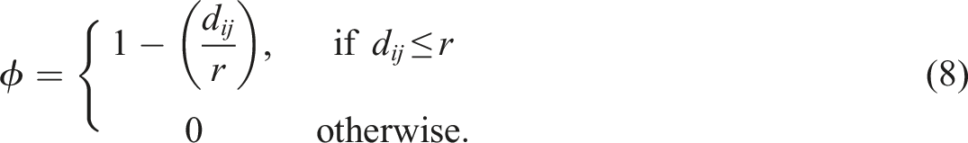
In each metropolitan region, we proceed by creating two different spatial weights matrices by varying the way distance is measured between observations. In both matrices, the proximity-weighting function ϕ is a simple linear decay (triangular kernel) encoding a spatial weight that decreases with distance up to a threshold of 2 km, outside of which observations no longer have an effect, (that is, r = 2000)
Between the two W matrices, however, we vary the input distance matrix D, between two concepts, Euclidean distance (W
euc
) and network distance (W
net
), where network distance is defined as the shortest path along the pedestrian transportation network. In both matrices, the diagonal is set to one, indicating that there is no spatial discount for the value located at observation i. Using these weights matrices W
net
and W
euc
to build local environments for each metropolitan region, equation (1) propagates the two constructs through equations (2)–(6), yielding two segregation measures
Inferential framework
We assess the importance of considering network distance in segregation measurement by adopting the inferential framework outlined in Rey et al. (2021b) and Cortes et al. (2020). The framework leverages a computational approach to statistical inference using random labeling to compare the observed difference between the two segregation measures (network vs Euclidean) to a counterfactual distribution of differences generated from the same data. More specifically, the measures
We then create two synthetic datasets by pooling the input units from both original datasets and reassigning them at random. For each block group, we randomly reassign the labels (net, euc) to the observed spatial lags from equation (2). Once all units have been assigned to a group, the segregation measures are re-computed and their difference taken. This process is repeated 10,000 iterations. By comparing the observed difference in the two segregation measures against a distribution of differences generated via synthetic datasets, we are able to develop inferential statistics using a conventional t-test. Our test, in this case, adopts the null hypothesis that distances come from a common distribution and thus the expected difference in the segregation measures is 0. The p values represent the probability that, under the null, a simulated difference is greater than the observed difference
Network distance is an important consideration
Although the Pearson correlation between planar and network-based segregation measures is ρ = 0.987, our results provide clear evidence that the choice of appropriate distance metric plays an important role in the computation of a spatial segregation index. We highlight this result using the fact that applied segregation research often uses ordinal rankings to describe and compare the magnitude of segregation across a set of places. While still high, the rank correlation between the two measures is considerably lower at τ = 0.90. Substantively, this means that an analysis of segregated metropolitan regions will result in different conclusions regarding the “most segregated” places, depending on which distance measure is employed. A visual comparison of the top 15 most segregated metros is provided in Figure 2, demonstrating how different places exchange ranks, and Figure S3 in the supplementary material portrays the relationship between segregation measured using the two different distance metrics for the sample CBSAs. Planar versus network segregation rankings.
Descriptive statistics for segregation differences.

The distributions of both
Network characteristics and segregation differences
Metropolitan travel infrastructure as a network graph
The travel infrastructure in a metropolitan region serves as its skeleton for both urban development and social interactions. For decades, scholars have worked to quantify the aspects of urban form that help explain behaviors such as travel mode choice (Crane, 2000; Clifton et al., 2008; Ewing and Handy, 2009; Ewing and Cervero, 2010). A recent evolution of this work is the conception of a travel network as a formal graph structure (Araldi and Fusco, 2019; Boeing, 2018a, 2018b; Dibble et al., 2019; Fleischmann, 2018; Fleischmann et al., 2021) and a set of software tools that facilitate its analysis as such (Boeing, 2016; Fleischmann, 2019). Understanding the travel network as a topological graph provides a different picture of its accessibility structure and the way it facilitates interaction among residents (Levinson et al., 2017). Here our goal is to use these graph topology metrics to explain the variation we observe in
Measuring graph structure
Network topology metrics.
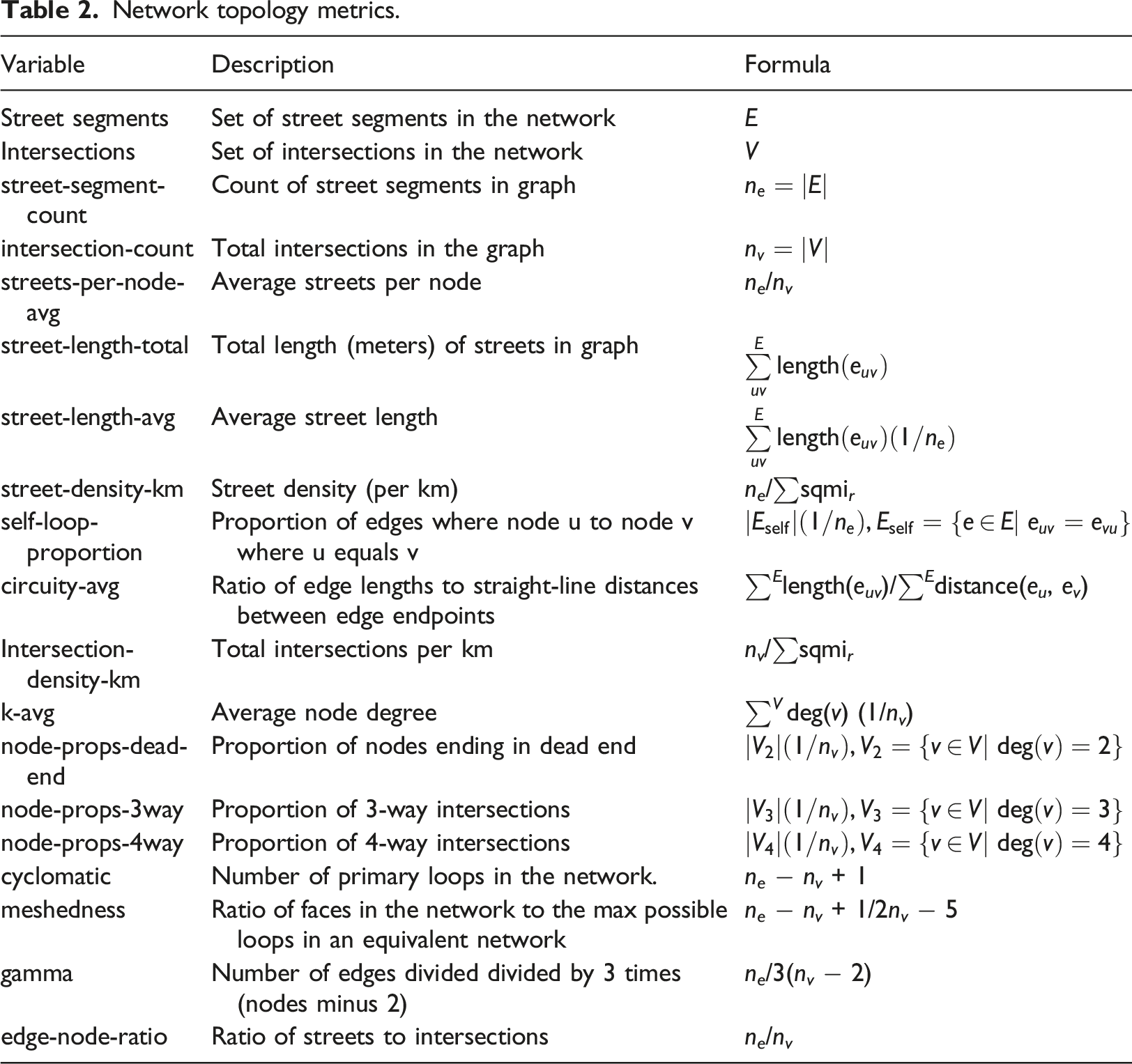
Cyclomatic complexity can be viewed as a measure of the network’s redundancy and its ability to provide alternative passages when a given route is blocked. According to Bourdic et al. (2012: 599), “the cyclomatic number represents the number of primary loops in the network. The greater the number of loops, the greater the number of possible routes in the city… it is more efficient to propose a multiplicity of smaller roads so users can choose and spread over these paths, which are ultimately better suited to the variety of their destinations. The cyclomatic number refers to this multiplicity of loops that increase the number of possible paths. In a public transport network with a high cyclomatic number, a failure in one station will not freeze an entire zone.” As such, we would expect that an increase in cyclomatic complexity would reduce
The meshedness coefficient is “based on the notion of circuits (or faces), network regions enclosed by loops of linked edges and nodes (analogous to an urban block surrounded by streets) that provide alternate movement routes” (Feliciotti, 2018). Meshedness is the “ratio of the number of faces in the network to the maximum possible number of loops in an equivalent network with the same number nodes” (Fleischmann et al., 2022). Buhl et al. (2006) use the meshedness coefficient to assess the connectedness of a graph, and whether its configuration is closer to a tree-like network or to a maximally connected grid. As Feliciotti (2018) describes, “in strictly tree-like networks, origins and destinations are only linked via a single path, which means that users have only one choice of movement and any point failure in that route would cause major disruption on performance. In turn, grid-like networks provide many ways to get to a same place, greater choice for the user and reduced impact of point failure.”
In the example of Figure 1, the network in San Clemente Figure 1(a) is more tree-like than the gridded network in Chicago Figure 1(b), indicating that meshedness is higher for Chicago than San Clemente. This distinction is shown similarly in the stylized depiction of meshedness created by Feliciotti (2018) in Figure 3, with the lefthand diagram having a more tree-like structure and thus a lower meshedness coefficient than the diagram on the right. Given the clear difference between Figure 1(a) and (b), we would expect that greater meshedness would result in lower Stylized depiction of meshedness by Feliciotti (2018).
Circuity is a measure of the “windingness” of a city’s streets. It is a ratio of an edge’s network distance to the Euclidean distance between its starting and ending nodes. In stylized terms, it represents the difference between walking between any two intersections and flying between them. For example, a mountain switchback trail would have a higher circuity measure than a flight of stairs that connected the same two origins and destinations. The former would be easier to traverse because of its lesser slope, but the path would sacrifice greater distance traveled as a result. Here, our measure of circuity is the average taken over all edges in the network. All else equal, we would expect that a lower circuity measure would result in a lower
Graph topology and segregation differences
We begin with an exploration of correlation among different variables that characterize the graph topological structure, as well as the correlation between Clustermap of correlation structure in network metrics.
A second group of variables includes population, street length, cyclomatic number, and measures of street and intersection density. This component appears to measure the transportation graph’s complexity and size. The component may also reveal something about agglomeration and self-scaling, as the density measures appear to grow in tandem with size. A final third apparent grouping of variables includes circuity, and the proportion of self-loops, as well as three-way and dead-end intersections. This component is strongly negatively correlated with the first and appears to indicate network clogging or stoppages. It is interesting to note that circuity is positively correlated with the proportion of dead-end end streets. Notably each of the three measures under study (cyclomatic complexity, meshedness, and circuity) each belong to a different component, suggesting that our chosen variables each represent a distinct part of the network structure.
Figure S3 in the supplementary material portrays the pairwise correlations between the percentage difference in the two segregation measures and different properties of the networks in each of the CBSAs. The strongest correlation is between the percentage difference and the size of the difference in segregation. This indicates that the percentage differences are not an artifact of a small denominator problem, whereby low levels of planar segregation would result in even small differences between network and planar-based segregation to appear to be large. Focusing on the network properties, as the proportion of 4-way intersections increases, the difference between segregation measured using network and planar distances grows. Segregation differences also grow with the average node incidence, street length, edge length, and circuity of the network. In general, as the size of the network increases, the difference in the segregation measures decreases. The relative differences in segregation measures are negatively associated with the level of segregation in the city.
Modeling the difference between metrics

Segregation difference.
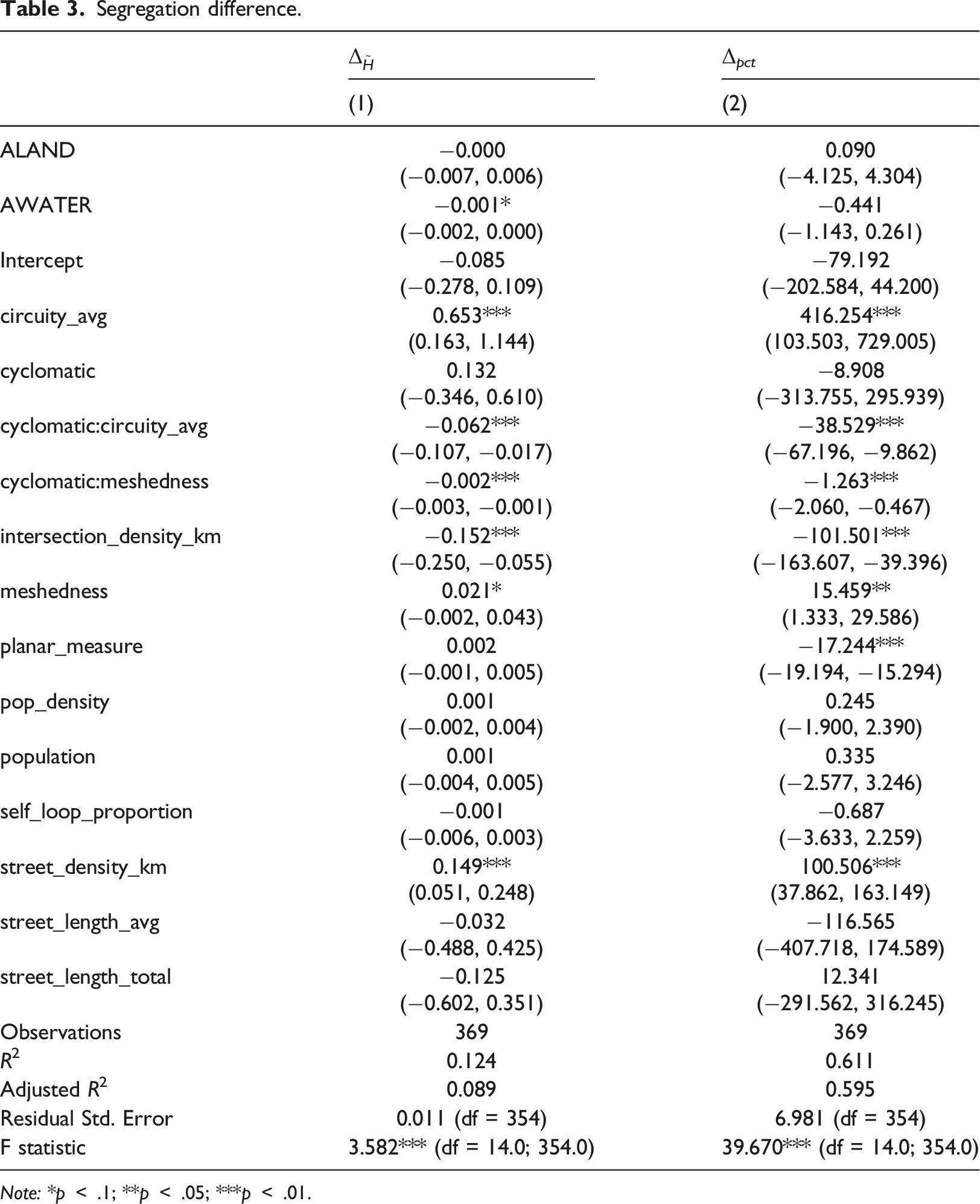
Note: *p
After removing collinear variables such as the share of proportions in different connectivity levels and other constructs well-captured by other variables (see Figure 4), our preferred models include a subset of network topology measures and interactions between cyclomatic complexity and (1) meshedness (2) circuity. In all specifications, these interactions significantly improved model fit. Moreover, the relationships between variables are generally consistent regardless which dependent variable is used. Right-hand side variables following a normal distribution are z-transformed and those following a power distribution are transformed via natural logarithm.
Regardless of the chosen dependent variable, the models display similar results, most of which are intuitive. Significant variables include the density of streets and street intersections, network circuity, and the two interaction terms. As expected, the coefficient for intersection density is negative, suggesting that as the number of intersections per kilometer increases, the gap between Euclidean and network-based segregation indices falls. This comports with intuition as greater intersection density leads to a network with greater ability to change direction, and thus a better approximation of unconstrained travel. Circuity is also positive and significant, suggesting that as streets get more winding and curvilinear, the distance between segregation indices grows. However, the interaction between cyclomatic complexity (a measure of redundancy in the network) and circuity is negative, which suggests that as the network offers more possible routes between an origin and destination, the effect of circuity falls. Again, this result is intuitive, as increased cyclomatic complexity offers more opportunities for short-cutting through a circuitous network.
One counterintuitive result is the weakly significant and positive coefficient for network meshedness. Taken at face value, this would suggest that networks with a regular grid pattern increase the distance between segregation measured on the network versus the same data measured on a plane. One possible explanation for this result is an inability of this relatively simple model to account for multiple interactions between meshedness, density, and complexity. While it is possible for a street network to have high intersection density, high street density, and low meshedness (such as a dense but highly dendritic subdivision), such networks are likely comparatively rare in major cities (or are difficult to capture at a metropolitan scale). In such a situation, some variation attributable to meshedness may instead be consumed by the competing coefficients for street density and network density. Exploring the complexity of these relationships is an important avenue for further work.
Discussion
There are two additional parameters worth exploring: the distance-decay function ϕ and the radius that defines the extent of the local environment r. In this paper, we adopt a simple linear decay function, but others such as Gaussian and exponential decay functions are applied regularly in both the segregation and spatial interaction literature. Our initial explorations suggest that our findings are robust to the choice of decay function, but future work could explore this issue in greater detail. Further work could also explore the choice of neighborhood radius r. Here we adopt the one-mile radius as a reasonable specification of the neighborhood, but we may obtain different results by choosing a different threshold, particularly when analyzing large heterogeneous networks.
Notably, by varying the r parameter and recalculating the segregation indices presented here, it is possible to generate a network-based version of the “multiscalar segregation profile” introduced by Reardon et al. (2008), which would provide additional insight into the way that networks may affect multiple scales. In Figure S4 in the supplementary material, we recreate a graph by Roberto (2018) showing the network-based multiscalar profile for Pittsburgh, PA using our data and methodology. After the critical distance of about 1 km (which provides travel outside a given blockgroup) the difference between network and Euclidean profiles is roughly constant. Again, this initial exploration suggests our results are likely robust to choice of r, but this finding should be subject to further scrutiny.
There are also other ways researchers could partition or conceptualize the street network graph for further study. In this example, we include a simple set of graph-wide summary measures, for example, meshedness, average degree, and circuity. These metrics could also be measured for different “spatial scales” of the network, that is, different subgraphs (e.g., using the same distance threshold used to define r). Summarizing these measures and using them as input to the regression model would provide a different picture of the relationships; it would also facilitate the inclusion of other commonly used graph metrics, such as closeness centrality or betweenness centrality. The significant interaction effects we uncover between meshedness and cyclomatic complexity and circuity and complexity also suggest that this is a ripe avenue for further research. In these cases, the significant interaction effects are likely created by heterogeneity in large travel networks, and more refined measures of subgraphs (rather than aggregate summaries of the entire network) may help uncover important localized patterns.
There is also a second issue of spatial scale, which is that here we examine all relationships at a metropolitan scale. Because housing and labor markets are regional in scope, segregation analysis is natural at the metropolitan-level, but adopting such a large scope may obscure important intra-metropolitan variation. For example, metropolitan regions have typically been developed over several distinct time periods, each of which may reflect a particular urban design paradigm or growth management strategy. Since the network measures computed here are averaged over the entire metro region, there may be utility in examining how suburban networks differ from urban ones. Decomposing the urban areas or adopting a multilevel modeling framework could help examine these nested structures.
Conclusion
In the segregation literature, the importance of space has long been recognized, but a full grasp of its implications still eludes researchers. In this paper, we show that when considering the role of transportation infrastructure in segregation measurement, we obtain substantially different results than classic spatial approaches that adopt Euclidean measurements. More specifically, we show that when ignoring the connectivity of local travel networks, the spatial information theory index
Put differently, we show strong evidence that this bias is prevalent in a large share of cases. When examining all metropolitan CBSAs in the United States, between 14% and 25% of the areas show a statistically significant difference. This result provides new insight into the importance of considering the built environment when conducting spatial analysis in general, and measuring segregation, in particular. By leveraging advances in both network routing algorithms and statistical methods, we analyze metropolitan regions in the United States at a massive scale, finding the shortest routes through millions of street intersections to provide concrete evidence of a widespread phenomenon first suggested by Roberto (2018).
After demonstrating the importance of considering travel infrastructure in segregation measurement, we proceed by measuring the topological characteristics of the pedestrian travel network in each metro region, and assessing their relationships with the observed differences in segregation. We show that many measures of the graph structure are highly intercorrelated, and only a few metrics are necessary for capturing a reasonable picture of the large-scale graph structure. Following, we find that the most important characteristics in the network are intersection density, which reduces the difference between network and Euclidean measurements, and the circuity of the street network, which increases the difference. Together these findings suggest that network design decisions like ensuring dense and interconnected street grids that adopt straight edges and avoid circuitous patterns can help reduce the segregation measured in metro regions. Nevertheless, the significant interaction effects in the models also suggest more research is necessary to fully understand the effects of heterogeneous network patterns.
In future work, this research could be extended in several directions. One promising avenue is the consideration of alternative impedance measures when calculating shortest-path distances along the travel network. In the present study, we assume a constant rate of travel consistent with the average walking pace, and that impedance is reflected by graph distance alone. Alternative constructs could include elevation along with distance to get a more complete measure of the effort required to traverse by foot or bicycle. Future work could also examine the impacts of other ways to conceive of the “pedestrian” network structure, such as including parks, paths, and trails rather than sidewalks and footpaths included in OSM. Similarly, the travel network could also be extended to include public transportation or (potentially congested) automobile travel. These considerations would require extensive additional data, which may limit the capacity for cross-sectional comparisons, but would also provide insight into alternative concepts of space and distance. They would also provide additional robustness checks against the results here to understand whether the same relationships hold for transit and automobile network, which have considerably different graph properties (Boeing, 2018b).
Another important avenue for further work is the blending of multiple graphs for a more complete understanding of multi-contextual segregation. For example, children who live in a given neighborhood are simultaneously embedded in local neighborhood contexts, school catchment boundaries, and other local institutions such as religious and community organizations. Each of these contexts have partially overlapping, occasionally nested, and often imperfectly defined geographic boundaries, a full synthesis of which requires the development of new methods that integrate across these contexts (Galster, 2001, 2019). As one example, Wolf (2021) provides a technique for blending multiple graphs together, one spatial and one aspatial, and similar methods could be possibly used to integrate multiple contexts. Work along these lines would also help address the call by Reardon and O’Sullivan (2004: 156) for metrics that help understand bridges across social networks.
An understated but important contribution of this work is its attempt to bridge the gap between spatial segregation measurement and other areas of spatial analysis. By formulating a spatial segregation index in terms of a spatial lag operator common in spatial econometrics, we hope to foster a greater dialog among researchers in urban social science regarding the most satisfactory ways to encode spatial relationships from both theoretical and methodological perspectives. Given the results presented here, we believe the appropriate operationalization of space remains a clear hurdle for understanding social interaction and urban inequality. Thus, we close with a classic reminder from a legendary scholar in spatial analysis, that “it remains for spatial analysts to carefully specify spatial weights matrices so that they truly represent the phenomena being analyzed” (Getis, 2009: 409). In the context of segregation measurement, it is clear that ignoring intentionally designed aspects of the built-environment skews our concept of social interaction.
Supplemental Material
Supplemental Material - Segregated by design? Street network topological structure and the measurement of urban segregation
Supplemental material for segregated by design? Street network topological structure and the measurement of urban segregation by Elijah Knaap and Sergio Rey in Environment and Planning B: Urban Analytics and City Science
Footnotes
Declaration of conflicting interests
The author(s) declared no potential conflicts of interest with respect to the research, authorship, and/or publication of this article.
Funding
The author(s) disclosed receipt of the following financial support for the research, authorship, and/or publication of this article: This work was supported by the Division of Social and Economic Sciences (1831615).
Data availability statement
Supplemental Material
Supplemental material for this article is available online.
Notes
References
Supplementary Material
Please find the following supplemental material available below.
For Open Access articles published under a Creative Commons License, all supplemental material carries the same license as the article it is associated with.
For non-Open Access articles published, all supplemental material carries a non-exclusive license, and permission requests for re-use of supplemental material or any part of supplemental material shall be sent directly to the copyright owner as specified in the copyright notice associated with the article.