Explainable spatially explicit geospatial artificial intelligence in urban analytics

Abstract

Geospatial artificial intelligence (GeoAI) is proliferating in urban analytics, where graph neural networks (GNNs) have become one of the most popular methods in recent years. However, along with the success of GNNs, the black box nature of AI models has led to various concerns (e.g. algorithmic bias and model misuse) regarding their adoption in urban analytics, particularly when studying socio-economics where high transparency is a crucial component of social justice. Therefore, the desire for increased model explainability and interpretability has attracted increasing research interest. This article proposes an explainable spatially explicit GeoAI-based analytical method that combines a graph convolutional network (GCN) and a graph-based explainable AI (XAI) method, called GNNExplainer. Here, we showcase the ability of our proposed method in two studies within urban analytics: traffic volume prediction and population estimation in the tasks of a node classification and a graph classification, respectively. For these tasks, we used Street View Imagery (SVI), a trending data source in urban analytics. We extracted semantic information from the images and assigned them as features of urban roads. The GCN first provided reasonable predictions related to these tasks by encoding roads as nodes and their connectivities and networks as graphs. The GNNExplainer then offered insights into how certain predictions are made. Through such a process, practical insights and conclusions can be derived from the urban phenomena studied here. In this paper we also set out a path for developing XAI in future urban studies.

Keywords

Urban analytics graph neural networks explainable AI geospatial artificial intelligence road networks

Introduction

The increasing awareness of open data initiatives for building smarter cities (Neves et al., 2020) has brought about a ‘digital turn’ into urban studies (Ash et al., 2018). Thanks to the abundant data now available, modern urban analytics seeks advanced technologies, and dedicated models and algorithms, to support better city governance with detailed analysis to aid urban planning processes that tackle socio-economic and environmental problems (Lei et al., 2023b; Wang and Biljecki, 2022; Liu and Biljecki, 2022; Song et al., 2022; Yossef Ravid and Aharon-Gutman, 2022; Kang et al., 2019; Carra and Barthelemy, 2019; Yeh, 1988).

Graph neural networks (GNNs) are an example of a type of geospatial artificial intelligence (GeoAI) method that has proliferated in urban analytics (Zhu et al., 2018; Li, 2020; Janowicz et al., 2020; Liu and Biljecki, 2022; Mai et al., 2022b, 2022a). Given their ability to intuitively encode spatial locations, dependence and heterogeneity from spatial and spatio-temporal data, GNNs are often interpreted and employed as a spatially explicit GeoAI approach to address the question of ‘what is special in spatial?’ (Mai et al., 2022b; Liu and Biljecki, 2022). In urban studies, GNNs have been shown to outperform conventional models in many tasks, for example, in urban place understanding (Zhu et al., 2020), urban social sensing (Liu and De Sabbata, 2021), traffic analysis (Zhao et al., 2022; Xiao et al., 2021), and urban dynamics (Zhang and Cheng, 2020; Pagani et al., 2021).

However, along with the success of developing advanced spatially explicit GeoAI methods, the interpretability and explainability of deep learning methods in general, and GNNs for urban studies in particular, have become imperative issues that need to be addressed (Krishnan, 2020; Liu and Biljecki, 2022). Why does the model deliver spatial analysis results in a specific manner? If the model produces expected and good results, do we know why and how to leverage them further? In the context of urban studies, the spatial process of socio-economic activities, for example, gentrification, urban growth or even everyday urban population flows, is often a result of joint actions. Whereby one area may go through specific changes or dynamics, neighbouring areas can be affected by that process independently or in conjunction with other factors (Reades et al., 2019). While GNNs have proven to be useful by leveraging the interactive nature of spatial processes, the internal mechanism of how a spatial process has impacted the model performance, as well as how to utilise the model interpretability to gain further insights into urban phenomena, remain underexplored.

This paper aims to exploit the explainability of AI models to better support urban analytics. Explainable AI (XAI) is a set of methods that seeks to enable humans to understand the decisions or predictions conducted by the AI, which serves as a potential tool to address the questions mentioned above (Liu and Biljecki, 2022; Shi et al., 2022). However, there are only a handful of urban research studies that are working in this direction. Many of them fall in the domain of Transportation for traffic management and engineering-oriented purposes (Li, 2023; Wagner et al., 2022; Nascita et al., 2021a, 2021b), or there are other studies that have conducted XAI research with street view images (SVI) to study the street environment (Liu et al., 2023; Xie et al., 2022; Lee et al., 2022; Thakker et al., 2020) or worked with satellite images to improve the understanding of urban environments (Abdollahi and Pradhan, 2021; Vinuesa and Sirmacek, 2021) but the methods adopted have been non-spatial. To the best of our knowledge, despite the recent trends in spatially explicit GeoAI development, no research has been conducted using XAI that can encode spatial information in its computation process to understand urban phenomena better. This may be because the development of spatially-explicit GeoAI in urban analytics is still in an early phase (Liu and Biljecki, 2022); thus, previous research has focused more on the usability of the models rather than the explainability. Moreover, XAI is regarded as a new research theme that is still underdeveloped. For example, much of the current XAI development has contributed to the field of computer vision, where convolutional neural networks have played a vital role (Ahmed et al., 2022) while very few efforts have been devoted to GNNs.

The need for studies of XAI in urban analytics represents both a challenge and an opportunity for investigating such a line of research. Here, we propose an urban analytical method using a well-developed GNN-based XAI method called GNNExplainer (for a detailed explanation, see Section Background) (Ying et al., 2019) to understand urban geographical phenomena better. Given the nature of GNN-based methods that explicitly encode spatial locations as graphs for their computational process, we consider GNNExplainer to be a spatially explicit XAI. We propose two case studies that focus on urban traffic analysis and population research combining SVI, a trending data source in urban analytics (Biljecki and Ito, 2021), and GNNs to exploit the potential of the XAI.

In this paper,

• we propose an analytical method that combines GCNs and GNNExplainer, offering both predictive power and explainability regarding the urban questions under investigation;

• we explore the use of GNNExplainer in urban analytics, and we open up a new path of employing spatially explicit XAI methods to study urban-related questions;

• we discovered that XAI methods can provide not only explanations of the GeoAI models adopted but also help to gain insights into how certain urban phenomena occur.

We hope this paper will promote the use of XAI in urban analytics and inspire further studies and innovations in this field.

Background

Graph neural networks in urban analytics

GNNs are a genre of deep learning methods that infer graph-structured data in the form of an adjacency matrix (where 1 denotes a connection and 0 represents non-adjacency). The key idea behind GNNs is the local convolution process that leverages information from the neighbourhood of each node in the graph to update its own representation. As such, information can flow across the graph, enabling nodes to learn from their local connectivity patterns and the overall graph structure. This creates a solid connection to geography because the use of various measures to define the geographical units (e.g. neighbourhood, points/areas of interest) and its conceptualisation as a graph network (i.e. using spatial weights) has long been one of the core approaches in geographical information analysis (O’Sullivan and Unwin, 2010). Therefore, the use of GNNs is proliferating in spatial data analysis. Given their ability to encode locations as graphs, GNNs and many of their variants have been widely considered as one of the most successful spatially explicit GeoAI applications used for spatial analysis (Mai et al., 2022a, 2022b; Liu and Biljecki, 2022; Li, 2020; Janowicz et al., 2020). Among GNNs, Graph Convolutional neural Networks (GCNs) (Welling and Kipf, 2016) are widely adopted for urban analytics (Liu and Biljecki, 2022). As shown in Figure 1, GCNs contain filters that perform graph-level convolutions over the graph to aggregate node information and produce meaningful embeddings (i.e. numerical representations of the data) through the learning process, which can be employed for downstream tasks, such as classification, regression, etc. In our study, the GCN node-level and graph-level classification abilities are the main focus.

Figure 1.

An example of a Graph Neural Network (GNN) in urban analytics, adapted from Liu and Biljecki (2022). The urban spatial objects, events or phenomena under study need to be conceptualised as a graph structure. The GNN model will take advantage of the constructed graph by using a convolution approach (different ways can be adopted subject to the model architecture) to pass, aggregate, and adapt information among nodes based on their adjacency to other neighbouring nodes. Hence, each node in the graph learns locally. Through such a learning process, the GNN learns meaningful vector representations (i.e. embeddings) via the nodes, which can be used for downstream tasks, such as classification and regression.

GCNs have been used for a wide range of applications in urban analytics, from socio-economic studies to urban sustainability (Zhang et al., 2022; Liu and Biljecki, 2022; Zhu et al., 2022; Gao, 2021). This article is not intended to provide a detailed literature review of GCN-based applications in urban studies. Instead, we highlight only a few studies to present the broad usability of GCNs and thereby lay down the foundation for our showcase studies (see Section 4).

Studies of traffic forecasting may be among the first beneficiaries of advanced GCN development in urban studies. The intricate nature of urban road networks can be easily modelled through graph structures and fed into a GCN model. Fan et al. (2020) and Jiang and Luo (2022) surveyed an exhaustive list of literature for recent traffic-related research and identified that GCNs are at the frontier of deep learning-based traffic prediction research. Most of the literature in this domain has focused on analysing road-level traffic flow, primarily traffic volumes (e.g. Chen et al. (2020); Cao et al. (2020); Xu et al. (2020); Zhao et al. (2022)). GCNs and their variants have been shown to provide accurate predictions by capturing the spatial and spatio-temporal dependency of the road networks; however, as mentioned in Section 1, studies are currently focused more on the usability of the model instead of offering interpretability and explainability regarding how the GCN made the prediction.

Another interesting topic yet one with less involvement of GNNs is urban population studies. Unlike traffic analysis, which is often conducted at the road level, urban population focuses on the region or neighbourhood level. Existing research has identified a strong correlation between the urban population distribution and various road networks (Wang, 1998). A high density of urban road networks correlates with higher urban population density and vice versa. However, as the use of spatially-explicit GeoAI for such a socio-economic-oriented research objective is still in an early research phase (Liu and Biljecki, 2022), only a few studies have estimated urban population using GCNs (Xu et al., 2021; Yang et al., 2021). In this study, although we are not thoroughly investigating the use of, or developing specific, GCNs in urban population estimation, we aim to shed light on this topic (see Section 5.2).

Road networks and street view images

To explore the use of spatially explicit XAI in urban analytics, we define the unit in this study to be road networks in the city area. We conceptualised the road networks as a graph representation, fed the data into a GCN, and used GNNExplainer (see Section 3.2) to interpret the model performance and the results.

Thanks to the rapid development of computer vision techniques, image segmentation using SVI is now one of the predominant applications used to gather visual understanding of the urban environment, solve urban issues and support quantitative computational analysis of urban phenomena (Hou and Biljecki, 2022). Image segmentation aims to locate objects (buildings, roads, greenery, etc.) and detect their boundaries (lines, curves, etc.) to provide a semantic understanding of all objects included in an image. Such an objective is crucial in the quantitative characterization of the urban environment, particularly where traditional qualitative observation is not feasible. Image segmentation has been extensively used to support a wide range of analyses, such as urban traffic forecasting (Yin et al., 2015; Den Braver et al., 2020; Yao et al., 2018) and socio-demographic analyses (e.g. of population) (Goel et al., 2018; Deng et al., 2020). A typical example of image segmentation used in urban analytics is Cityscapes (Cordts et al., 2016), which is a benchmark data set that provides 30 categories of road objects (trees, roads, buildings, pedestrians, etc.) captured in the SVI. In our study, a deep learning model trained on the Cityscapes data set plays a vital role in supporting the comprehensive understanding of road networks; a detailed introduction is elaborated in Section 4.

Methodology

Figure 2 shows the proposed analytical method, which contains two components: a GCN for inference and GNNExplainer for the interpretation of the model and the results. Note that in this paper, our aim is not to deliver novel methods for urban studies. Instead, we combined two state-of-the-art methods to investigate how to semantically interpret the machine-oriented explanations provided by GNNExplainer on the predictive model GCN in an urban context. More details are provided in the following subsections.

Figure 2.

Proposed analytical method. The urban map has been downloaded from https://free-vectors.net/(creator: Ilya Sedykh), under license CC BY 4.0.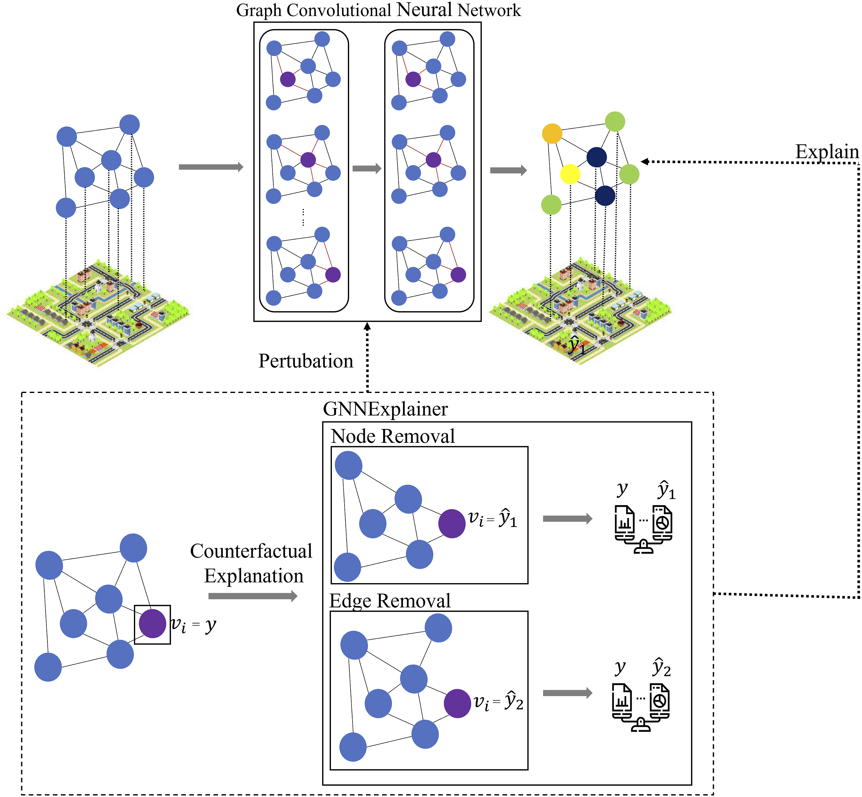

Graph convolutional neural network

Our method employs the two-layer GCN model developed by Kipf and Welling (2016) for the traffic and population (see Section 4) inference tasks. This GCN is also one of the most successful AI models, and has been adopted in a wide range of tasks solving urban issues, such as urban social sensing (Liu and De Sabbata, 2021; Zhu et al., 2020), travel demand forecasting (Zhao et al., 2022; Xu et al., 2020), and urban population flow studies (Li et al., 2021). The primary objective of the GCN is to generate a node representation by aggregating information from its own features and the features of its neighbours. Such a process is conducted through spectral-based convolutions over nodes in a graph that is defined as

g_{Θ} * x = U g_{Θ} U^{T} x

(1)

where g_Θ represents the convolution kernel parameterised by

Θ \in R^{N \times N}

in the Fourier domain. The kernel is randomly initialised from a Gaussian distribution and is then adjusted through the process of forward-and-back propagation in the GCN’s training phase. In other words, a kernel is a matrix that goes through the nodes in the graph (i.e. street networks in our paper), and extracts and aggregates information from the SVI-based urban features x. U is the eigenvector matrix of the normalized Laplacian matrix L = I_N − D^−1/2AD^−1/2, where A denotes the adjacent matrix of the graph (i.e. street network), I_N is the identity matrix and D is a diagonal matrix composed of node degrees.

The node representation generated through the graph convolution process can be used for both node- and graph-level classification. Node classification is defined as a set of tasks that predict the classes of unlabelled nodes based on other nodes, which are widely used in urban studies (Liu and Biljecki, 2022; Mai et al., 2022b; Janowicz et al., 2020). Graph classification as a task to predict graph labels based on graph structures and node features is less commonly seen in the existing urban analytics literature. While classification is not necessarily the primary focus of this paper, our study will explore the use of graph classification in urban population estimation (see Section 4).

GNNExplainer

GNNExplainer was developed by Ying et al. (2019) as the first XAI method for GNNs. It is a perturbation-based method that studies the output variations of different input perturbations on the model (Yuan et al., 2022). An intuitive understanding of the GNNExplainer is a network that explains a GNN by reducing redundant information in a graph without direct impact on its decisions. To achieve such a goal, using node classification as an example, the GNNExplainer generates a minimal graph that explains the decision for a node v and minimises the difference in the prediction using the entire graph and the minimal graph by maximising the mutual information (MI) through

\underset{G_{s}}{Max} M I (Y, (G_{s}, X_{s})) = H (Y) - H (Y | G = G_{s}, X = X_{s})

(2)

where G_s is the subgraph of graph G_original with associated features X_s. MI is the quantified changes in the prediction probabilities

\hat{y} = G N N (G_{o r i g i n a l}, X_{original})

, and H(Y) is the entropy term for the GNN predicted label distribution Y. Thus, to maximise equation (1), the network of GNNExplainer seeks to minimise the conditional entropy H(Y|G = G_s, X = X_s).

Figure 2 shows a simple example of how the GNNExplainer works. A GNN will first make predictions over the nodes of a given graph. GNNExplainer will then be applied to the GNN, seeking to explain why certain predictions were made. As shown in the figure, for a given node v_i with a predicted label y by the GNN, GNNExplainer will produce counterfactual explanations, that is, perturbations on the graph by removing other nodes or edges and generate subgraphs accordingly. Then, the GNNExplainer compares the new prediction $\hat{y}$ produced using the new subgraph with the original prediction y. If the changes in the nodes or edges significantly impact the original prediction, the counterfactual explanations are then valid and useful. Thus, the nodes or edges removed are essential for explaining the prediction of the targeted node. Through an iterative process, the GNNExplainer finds meaningful explanations for all nodes in the graph. Such explanations are different from conventional statistical approaches, which seek to investigate patterns (usually linear relationships). The explanation offered by GNNExplainer focuses specifically on the predictive model of the GCN used in this paper. In the rest of the paper, we will demonstrate that as long as the predictive model is robust, feature importance, together with other spatial interactions on the road network, can provide meaningful and interpretable insights into urban phenomena. It is also worth noting that the explanations offered by the GNNExplainer are the explanations of the GCN predictions, that is, machine-oriented outputs, rather than explanations coming from underlying urban theories. In Section 5, we will demonstrate how such explanations can be used for understanding urban contexts in a meaningful way with semantic-rich interpretations.

Study area

Our case study area is Wuhan, a metropolitan city in central China with a population of over 11 million. We collected four types of data that are used in this study: road networks derived from OpenStreetMap (OSM), one-day taxi travel data (collected on 3 July 2021), 2021 population statistics from the Wuhan Municipal Public Security Bureau, and panoramic SVI from Tencent Maps.

Data preparation

Figure 3 (left) shows 5075 roads collected from OSM. The GCN requires a graph representation of the data as input; thus, the road network in Wuhan was converted into a graph structure. Each road was considered a node, and its interconnection with other roads was formalised as the adjacency of the nodes in the graph. For example, if road A and B are connected in the road network, the nodes in the graph A′ and B′ will have an edge connecting each other. Figure 3 (right) illustrates the conceptualised graph, where such a graph is undirected (where all the edges are bidirectional).

Figure 3.

The road network and its conversion to a graph representation. Map sources: Esri, HERE, Garmin, INCREMENT P, © OpenStreetMap contributors, and the GIS user community.

As indicated in Section 2.2, SVI is now a vital data source for studying road networks and addressing urban issues. We collected 56,560 panoramic SVI taken from these roads in Wuhan from Tencent Maps. To study the road features, we used a pre-trained (with the Cityscapes data set as mentioned in Section 2.2) convolutional neural network (CNN) model DeepLabV3 (Chen et al., 2017) to semantically segment objects in each image into the following categories: Road, Sidewalk, Building, Wall, Fence, Pole, Lights, Traffic Signs, Trees, Grass, Sky Pedestrians, Cyclist, Cars, Trucks, Bus, Trains, Motocycle, and Bikes. The segmented results contained the proportions of each object in an image. Note that one road may have multiple SVI taken; therefore, we then aggregated the results by taking average values of each road object in all the SVI collected for a given road. Such aggregated results were used as node features in the conceptualised graph for further analysis.

Labelling

To demonstrate the use of XAI in urban analytics, we first employ a GCN on two widely studied areas of research. That is, we apply a GCN as a spatially explicit GeoAI to predict urban traffic volume (as a node classification task) and to estimate regional population (as a graph classification task) in Wuhan.

We added the volume of taxi travel data to the road networks, as shown in Figure 4 (left). We used Jenks Natural Breaks (Jenks, 1967) to classify the data into five categories (ranging from 0 to 4 in the maps), where these categories were employed as labels for the GCN to classify the nodes. Figure 4 (right) shows the Spearman rank correlation between the road features and the taxi traffic volume in Wuhan. The proportion of the roads and the broad field of view contributed by the proportion of sky in the SVI correlates the most with high urban traffic volumes. However, as an exploratory method, correlation gives an overall but limited insight to understanding such relationships further. In Section 5.1, we will demonstrate how XAI will enhance our understanding of how road features are linked to road traffic at a much higher resolution, allowing road-level inspection of the results. It is worth highlighting that the correlation analysis does not explain the GNN predictions nor interpret the results given by the GNNExplainer (i.e. importance scores, see Section 5). The statistical correlation between variables provided in this section is only a preliminary exploration of the variables, while GNNExplainer will be used calculate interpretability scores (i.e. importance scores) to measure the degree of feature influence on the predicted outcome of the model. We argue that such importance scores given by GNNExplainer have meaningful semantic information that helps us to quantitatively understand urban features and their potential impacts on urban phenomena (e.g. traffic and population volumes in this paper).

Figure 4.

Road traffic volume shown on the left and the correlation between traffic volume and different road features on the right. Map sources: Esri, HERE, Garmin, INCREMENT P, © OpenStreetMap contributors, and the GIS user community.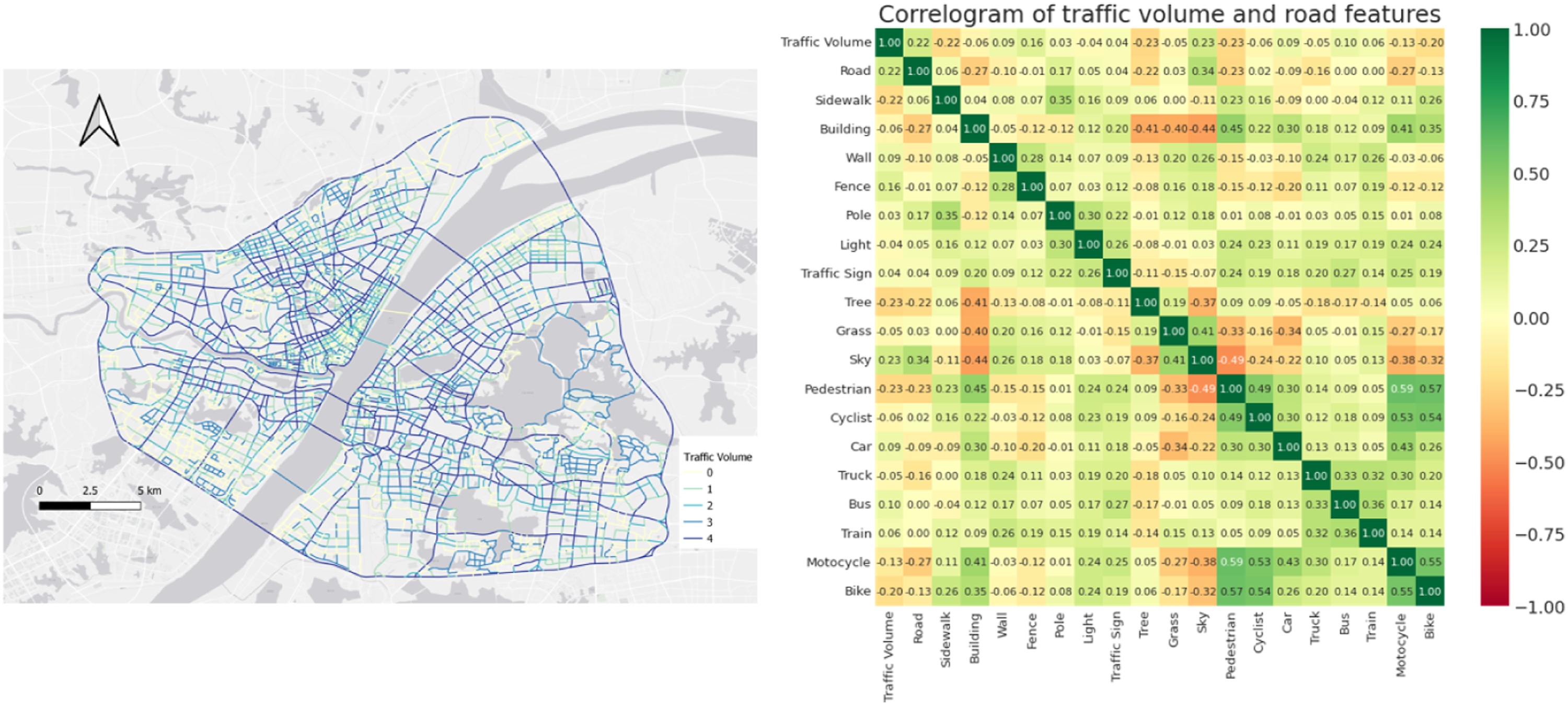

Figure 5 (left) shows population data collected from the census in 2019 for 881 neighbourhood-level sub-districts (so-called Jiedao, in Chinese, which is one of the smaller administrative divisions of urban areas in China) in Wuhan. Data for this task were collected from local authorities in Wuhan, China. The geographical boundaries of these local communities are then overlayed onto the road network to produce a set of graphs. Each graph has its own graph structure based on the connections of the roads inside each boundary, as shown in Figure 5 (right). The population in these local communities was also classified into five classes using the same Jenks Natural Breaks method and adopted as labels for the graph classification task.

Figure 5.

Population distribution in the study area on the left and the graph structure shown on the right. Map sources: Esri, HERE, Garmin, INCREMENT P, © OpenStreetMap contributors, and the GIS user community.

Understanding urban context

Gong et al. (2020) released a Chinese Essential Urban Land Use Categories (EULUC) data set that can be used to understand urban land use and human activities (Zhang et al., 2023). Figure 6 (left) shows the EULUC in Wuhan, which demonstrates identifiable patterns of where commercial and business, educational, industrial and residential land use is clustered and distributed. For example, commercial land use is largely clustered in the city centre next to the Yangzi River. In Section 5.1, we will use this as a base map to semantically understand the insights offered by using GNNExplainer on the road network.

Figure 6.

EULUC 2018, Wuhan (same colour palette used in Gong et al. (2020)) on the left and the 10 most important and dominant OSM road types in Wuhan on the right. Map sources: Esri, HERE, Garmin, INCREMENT P, © OpenStreetMap contributors, and the GIS user community. SVI extracted from Tencent Maps.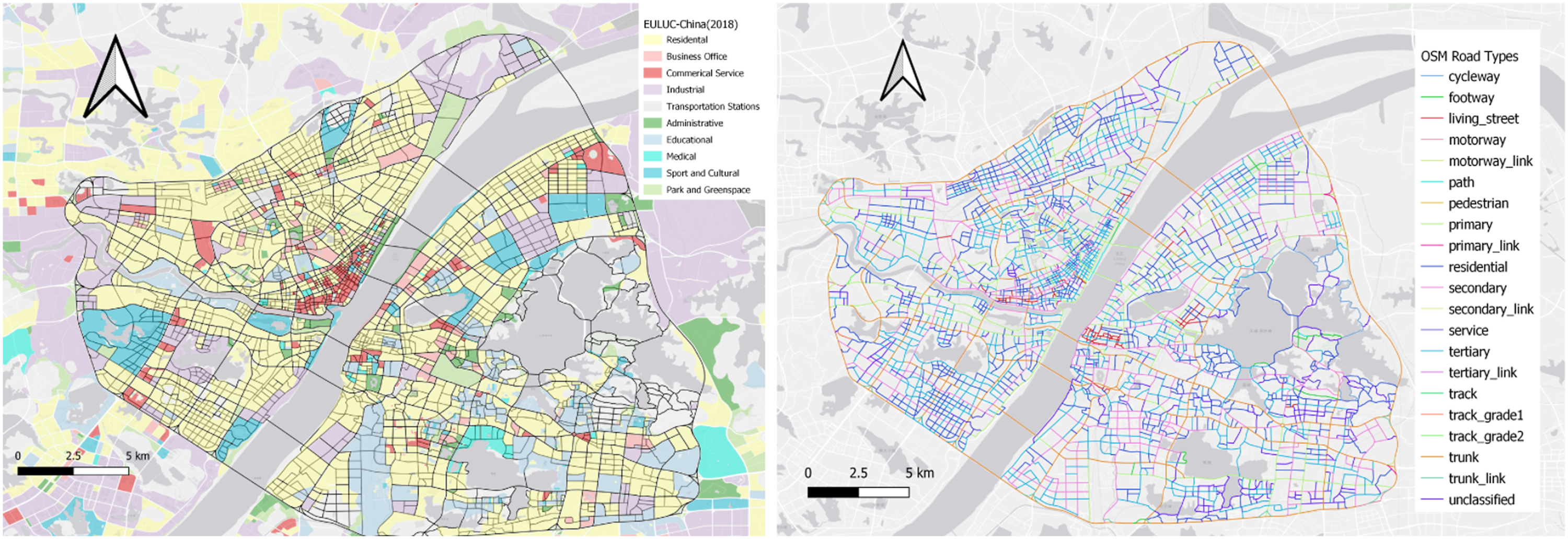

Figure 6 (right) summarises the dominant road types derived from OSM for Wuhan. These road types are defined by the OSM community (OpenStreetMap Wiki, 2022). The most important roads in the city that play a role in connecting inner-urban regions in the city are Motorway, Trunk, Primary, Secondary, Tertiary, Unclassified, and Residential. Other road types are named given their functions in the urban areas; for example, link roads connect roads and streets to the primary roads mentioned above, and Cycleway is for cycling activities. In Section 5.2, we will use such data to investigate how road types impact the population estimates of the local communities.

Experiments and results

The source code of this study was implemented using the Deep Graph Library (DGL) (Wang, 2019; Wang et al., 2019) with PyTorch (Paszke et al., 2019) as the back-end. We have provided our code on GitHub.¹

Explaining traffic volume

We formalised the traffic volume prediction as a semi-supervised node classification task. For the data prepared in Section 4, we randomly split 20% of the nodes from the data collected and processed as a training data set for the GCN model, while 10% were used for the model validation. The remaining 70% comprised the test data set for evaluating the model performance.

The GCN achieved an accuracy of 77.54% (averaged accuracy after running the model 10 times), which is in line with existing research that GCNs are helpful tools for studying urban traffic (Jiang and Luo, 2022). We then applied GNNExplainer on the GCN, using the model that achieved the best accuracy (78.9%). To explain such a process intuitively, we chose one road in Wuhan as an example. The selected road is part of Jiefang Avenue, one of the city’s primary and busiest roads, as shown in Figure 7 (left). The chosen road has 15 connections with other roads and was labelled by the GCN as four for traffic volume, representing the city’s highest taxi traffic volume level. Such a prediction is marked as correct because it is the same as the assigned label using Jenks Natural Breaks (see Section 4).

Figure 7.

Showcase of the results delivered by GNNExplainer. The road marked red is the selected road to be studied, and roads numbered from 1 to 14 are the interconnected roads. Our study seeks to explain why the selected road has the highest traffic volume by investigating which urban objects contribute to the traffic and how the road is impacted by the interconnected roads. Map sources: Esri, HERE, Garmin, INCREMENT P, © OpenStreetMap contributors, and the GIS user community. SVI extracted from Tencent Maps.

After making a valid prediction, GNNExplainer offered insights into why the chosen road was labelled as 4. GNNExplainer can explain a specific node prediction from two perspectives: first, how a node is impacted by its adjacent nodes (i.e. connected roads) through hops by giving scores to the connections (i.e. edges). Hops for a node are defined as its adjacency to other nodes in a graph; for example, one-hop neighbourhoods mean the direct adjacent nodes to the targeted node, and two-hop neighbourhoods are the nodes that are one hop away from the target node. In this article, we focused on the one-hop explanation of the target nodes. The second is to give importance scores to the node’s features (i.e. SVI-provided road features) to interpret which contributed the most to the prediction.

Figure 7 shows the results from GNNExplainer. The prediction of the selected road can be explained through the two perspectives mentioned above. From the road feature perspective, the Top-5 feature importance shows that the road objects Bus, Truck, Car, Building, and Road contribute the most to why the chosen road has the highest taxi traffic volume. Such a finding echoes existing literature and indicates that road traffic volumes positively correlate to the width of the roads (e.g. number of lanes), dense areas of buildings and easy accessibility to public transportation (Meng et al., 2017; Veloso et al., 2011; Phithakkitnukoon et al., 2010). From the road connection perspective, roads with numbers 13, 8, 14, and 9 contribute the most to the prediction. Mapping these roads onto the EULUC dataset, we can identify that the four roads connect diverse land uses where the residential areas that roads 13 and 8 traverse contribute the most to the high traffic volume of the selected road.

After a qualitative understanding of how GNNExplainer explains one road (i.e. node) in the road network, the next step is to quantify the interpretations of all the nodes in the conceptualised graph to understand the city’s traffic volume holistically. Table 1 summarises the results. The Average Top-5 Feature Importance Scores were calculated using the average scores of road features in each GCN predicted category (i.e. traffic volume). It shows the five features that have the largest impact on the predictions, which vary as the traffic volumes increase. For example, for the roads with the least taxi traffic, features such as pedestrians, cyclists, and walls have higher scores contributing to the predictions. Such a result aligns with the literature that those features commonly pose challenges to car driving (Morency et al., 2012). Meanwhile, wider roads (indicated by the score of Roads) and fields of vision (indicated by the score of Sky), and the appearance of other types of transportation (e.g. buses, trucks) contribute to the model’s understanding of high-traffic volume roads.

Table 1.

Quantitative insights provided by GNNExplainer applied to a model of traffic volume.

Traffic volume label	Average Top-5 feature importance scores	Top-3 EULUC land uses for interconnected roads
0	Pedestrians (0.7331), cyclists (0.7143), wall (0.6921), pole (0.6131), bike (0.5968)	Residential, educational, sport and cultural
1	Building (0.7892), fence (0.7123), pedestrians (0.6499), tree (0.6301), wall (0.5797)	Residential, medical, administrative
2	Grass (0.7481), motorcycle (0.7072), car (0.0.6626), light (0.6343), sidewalk (0.5551)	Residential, park and greenspace, commercial service
3	Car (0.7234), fence (0.6901), tree (0.6765), cyclist (0.6289), bus (0.5901)	Residential, unclassified, educational
4	Bus (0.7742), car (0.7029), road (0.6967), building (0.6813), sky (0.6026)	Residential, commercial service, industrial

The Top-3 EULUC land Uses for Interconnected Roads helps us to understand how the roads with certain traffic volumes are impacted by their connection with other roads by overlaying them on the EULUC map. The table shows that Residential areas contribute to all traffic volume categories. This is mostly because, as shown in Figure 6, residential areas occupy the largest proportion of the land use in Wuhan, considering it is the most populous city in central China. Industrial and Commercial Services contribute to the highest traffic volume, indicating that urban commercial areas attract high traffic demand. At the same time, industries seek roads that can carry high traffic volume to deliver products and raw materials. In contrast, due to the traffic control policies (Huang et al., 2012), roads that connect through educational, sports and cultural, medical and administrative areas contribute to lower traffic volumes. Note that in the cell for category 3, which represents relatively high traffic volume roads in the city, a type of road named Unclassified is shown in the table. Such roads are distributed in the areas that are not covered by EULUC, which contributes to a high traffic volume mostly because they are bridges and tunnels with high traffic volumes.

Through the study of traffic volume prediction, which was formalised as a node classification task, the GNNExplainer provides insights into how a road has a specific labelled traffic volume. We can derive a semantic understanding of traffic conditions by explaining and interpreting the results.

Explaining population in the urban environment

The population estimation was a graph classification task. As introduced in Section 4.1 and Figure 5, the graphs were created based on the 881 local communities and the road networks, resulting in 881 conceptualised graphs. During graph classification, 70% of the graphs were used for training the GCN, and the remaining 30% were used to test the performance. Similar to Section 5.1, we used Accuracy as the evaluation metric.

In such a graph classification task, the GCN achieved 59.2% accuracy (averaged accuracy after running the model 10 times) using the SVI segmented road features with the conceptualised graphs as inputs. Although the accuracy compared to the traffic volume prediction is much lower, we still consider such a model to be valid. Population estimation is a complicated task involving a wide range of factors (Wu et al., 2005), so using SVI features as inputs may only be proxies for some of these factors. However, to demonstrate the use of GNNExplainer, we simplified the task by only taking segmented features from SVI and road networks into account.

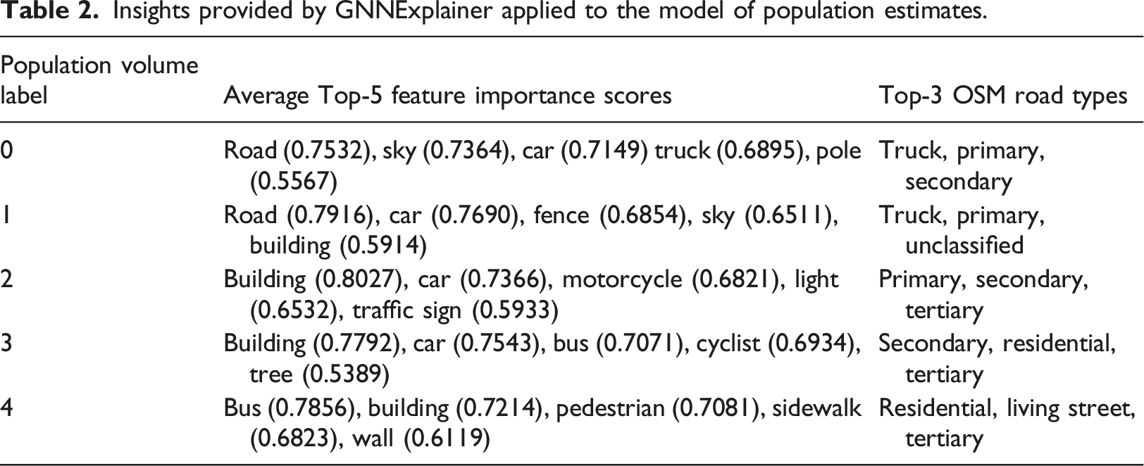
Like the node classification, we used the model that achieved the best accuracy (59.66%). GNNExplainer explains the graph classification from two perspectives: node features and graph structures. GNNExplainer gives importance scores for the node features by summarising all node features in one graph, aggregating the scores, and revealing which features contribute to a prediction for a graph. As in Section 5.1, we used the Top-5 Feature Importance scores to explore which features in SVI contribute the most to the population estimation. GNNExplainer gives importance scores for the graph structure to show which nodes (i.e. roads) contribute to the classification results. As introduced in Section 4.3, OSM organises roads into a hierarchical level of types. We investigated each graph to understand how road types for these dominating nodes contribute to the population estimation.

Table 2 summarises the results produced by GNNExplainer, and it is evident that with an increase in the population, which varies across the local communities, road features that play roles in the GCN estimation are different. For example, in less populated areas, which are located on the city’s outskirts (see Figure 5), roads that carry many cars are more important for the population estimation. At the same time, for comparably populated areas, the appearance of buildings, pedestrians and bus services become the decisive features for the corresponding labelling. Meanwhile, from the perspective of the Top-3 OSM road types, city trunk and primary roads, which function as connections through urban regions (Trunk, Primary, Secondary, and Unclassified), are more commonly present in the less populated areas. Moreover, residential paths and urban roads are in densely populated regions. Figure 8 shows two local communities that have the highest (Hubei University Community) and lowest (Zhuyehai Community) levels of population volume in the city, respectively. It is clear that Hubei University Community, as a populated area, has different road features and road types compared to Zhuyehai Community, which is less populated. It is particularly interesting that for the Hubei University Community, the predominant roads that help the GCN to learn the population level are those categorised as Residential in OSM. Such road types, together with road features of Pedestrian, Car, Sidewalk, and Cyclist in the Top-5 most important road features, help us to better understand the populated nature of such a community. Meanwhile, this qualitative inspection of the results echoes the findings in Table 2 that areas seem to share similar characteristics in each labelled population volume level.

Table 2.

Insights provided by GNNExplainer applied to the model of population estimates.

Population volume label	Average Top-5 feature importance scores	Top-3 OSM road types
0	Road (0.7532), sky (0.7364), car (0.7149) truck (0.6895), pole (0.5567)	Truck, primary, secondary
1	Road (0.7916), car (0.7690), fence (0.6854), sky (0.6511), building (0.5914)	Truck, primary, unclassified
2	Building (0.8027), car (0.7366), motorcycle (0.6821), light (0.6532), traffic sign (0.5933)	Primary, secondary, tertiary
3	Building (0.7792), car (0.7543), bus (0.7071), cyclist (0.6934), tree (0.5389)	Secondary, residential, tertiary
4	Bus (0.7856), building (0.7214), pedestrian (0.7081), sidewalk (0.6823), wall (0.6119)	Residential, living street, tertiary

Figure 8.

Showcase of the insights provided by the GNNExplainer in the population estimation task. The roads marked red represent the most dominating roads that contributed to the population volume. We use the Top-5 feature importance of the roads to investigate which urban objects may have a higher influence on the population volume and OSM dominating road types to understand the primary functions of the roads. Map sources: Esri, HERE, Garmin, INCREMENT P, © OpenStreetMap contributors, and the GIS user community. SVI extracted from Tencent Maps.

Bringing XAI into urban analytics

We have demonstrated that the interpretation and explanation offered by GNNExplainer can help us gain further insights into the urban environment. Here, we discuss how to further use the explanation offered by GNNExplainer and its potential use in urban analytics to support planning practices.

As introduced in Section 3.2, GNNExplainer is a perturbation-based XAI approach that learns which nodes and edges are essential for the predictions. The idea of perturbation is crucial as it facilitates an interactive process between a researcher and the urban phenomena being studied (Yap et al., 2022). Taking the Zhuyehai Community in Figure 8 as a naive example, we assume that the local government has a new agenda to attract more people to reside in this area. Based on our analysis in Section 5.2, two changes to the planning process could be recommended. Based on the results in Table 2, road objects that appeared more frequently in populated areas are Bus, Building, Pedestrian, Sidewalk, and Wall. Hence, we can increase the proportion of these road features within the community by 20% as well as decreasing other dominant features (Road, Sky, Car, Truck, and Light) by 10% as shown in Figure 8. The next step is to adjust the road networks so that they are more residential-friendly. Existing research has identified the importance of connectivity in the urban area to increase the population capacity (Koohsari et al., 2014; Stangl and Guinn, 2011). Thus, we added roads that purposefully connect trunk roads in the community with other roads, as shown in Figure 9. To add road features to these newly added roads, we synthesised the values by assigning the average road feature values of the existing roads (after the first step). Figure 9 demonstrates the process and the corresponding result. By implementing the two recommendations mentioned above, the population volume of Zhuyehai Community can be increased significantly as estimated by the GCN. Also, by using GNNExplainer on the result, we can identify that the newly added roads, which increased the connectivity of the area, contribute the most to the increased population.

Figure 9.

Showcase of the urban planning process using the proposed method.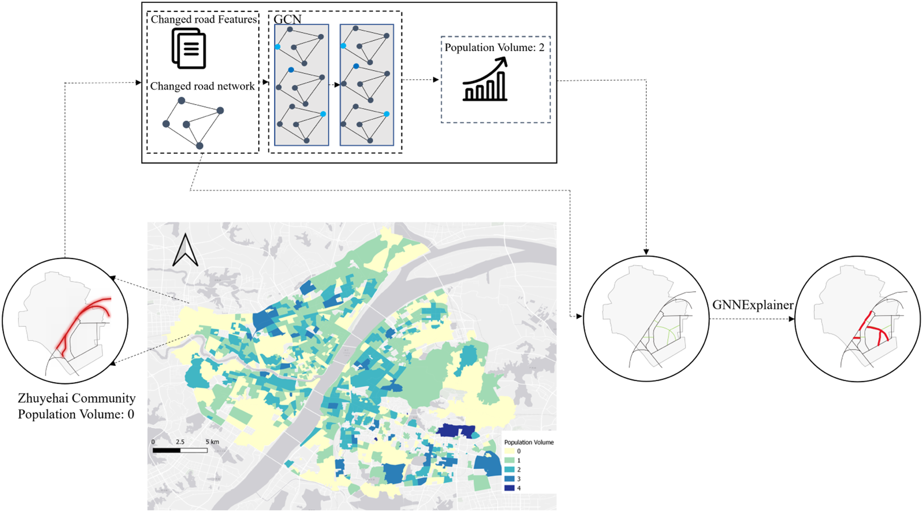

However, it is essential to note that such an example is naive, and is an oversimplified scenario compared to planning practice in real life. Nevertheless, our proposed method offers a preliminary exploration of the targeted planning objective. By leveraging the AI model that is now widely used in urban studies (As et al., 2022; Liu and Biljecki, 2022; Wang and Biljecki, 2022; Grekousis, 2019) and the XAI technology, our method offers both predictive power as well as interpretability of the model to understand the neighbourhood-level urban environment. As such, urban planners can use our method to adjust the features interactively and investigate the corresponding changes in urban phenomena quantitatively. Our model has the potential to be integrated with urban digital twins (Lei et al., 2023a, 2023b), where urban planners have the freedom to alter and simulate 3D-modelled urban objects based on the suggestions provided by our method.

Conclusion

Embracing the current ‘digital turn’ in urban geography, GeoAI-based models are increasingly being used to support a better understanding of the urban environment and aid planning processes. Most studies use the predictive ability of GeoAI models, but the desire to understand the model opens up a research agenda to develop explainable AI (XAI) models (Liu and Biljecki, 2022). Here we proposed an explainable spatially-explicit GeoAI method that offers both predictive power and the explanability of the results to gain further insights into the urban environment. Our method used a GCN to explicitly encode location information as a graph structure, contributing to its powerful predictive ability. Then in combination with the XAI model GNNExplainer to interpret the model’s predictions, we provided a road network and region-level understanding of the environment.

We demonstrated our proposed method in two examples of urban analytics: traffic volume prediction and population estimation in the tasks of a node classification and a graph classification, respectively, supported by SVI and the semantic segmentation of the images. The GCN first provided reasonable predictions by encoding the roads as nodes with segmented SVI as the features and their structures and connectivity as graphs. Such a finding supports the finding that SVI is an increasingly important data source for urban analytics (e.g. traffic and socio-economics) (Biljecki and Ito, 2021). Then, GNNExplainer offered insights into how certain predictions are made. For example, road features such as Road, Sky, and Car mostly dominate in high-traffic roads but less populated communities. Other features such as Pedestrian, Cyclist, and Buildings are primarily found in highly populated communities but in areas with low traffic roads. Furthermore, we provided an example of integrating our XAI method into an interactive urban planning process, demonstrating the potential use of our method in a real-world application.

However, we would like to highlight that GNNExplainer is considered a machine-oriented XAI model like the vast majority of existing XAI methods (Agarwal et al., 2023; Hsu and Li, 2023; Antoniadi et al., 2021). That is, the explanations (i.e. importance scores) given by the model only focus on the model-level predictions. Here, we attempted to give semantic meaning to the importance scores in explaining two urban phenomena. Although this enables the machine-oriented explanation to be human-oriented to a certain extent, it still keeps humans out of the loop in the automated explanation process. Plausible XAI methods, which are now commonly seen in Computer Vision (Kenny and Keane, 2021; Linardatos et al., 2020) where the generated counterfactual can be manipulated by humans, could be a solution towards solving this dilemma; however, it is rare to see such developments in graph-based deep learning methods. In the future, we will extend GNNExplainer to convert the model from a fully model-driven automated explanation process into a plausible human-oriented, interactive XAI model.

In the future, we plan to pursue this research as follows. First, because of the dynamic nature of urban phenomena, an increasing number of studies are adopting modified GNN models to capture the spatial and temporal dependency of the spatial objects (Zhao et al., 2022, 2023; Bui et al., 2021). In the future, we aim to extend the GNNExplainer to interpret spatio-temporal GNN models. Secondly, the road features and graph structure modifications were design choices, overlooking the spatial dependencies among the features and road networks. In the future, we will integrate geographically weighted regression to holistically adjust the road features and road networks by considering the spatial dependencies of the roads. Thirdly, the current graph structures were constructed based on the road connections in the form of undirected graphs. Such graphs neglect many other functional road characteristics that can be encoded in the conceptualised graphs, for example, road types and width, the direction of the roads (one-way or two-way), road conditions (e.g. age) etc. In the future, we will integrate and utilise these types of road characteristics to enrich the semantic information of the graphs.

Footnotes

Acknowledgments

We appreciate the comments by the editor and the reviewers. We thank the members of the NUS Urban Analytics Lab, Building and Urban Data Science (BUDS) Lab, and Integrated Data, Energy Analysis + Simulation (IDEAS) Lab for the discussions. This research is part of the project Multi-scale Digital Twins for the Urban Environment: From Heartbeats to Cities, which is supported by the Singapore Ministry of Education Academic Research Fund Tier 1.

Declaration of conflicting interests

The author(s) declared no potential conflicts of interest with respect to the research, authorship, and/or publication of this article.

Funding

The author(s) disclosed receipt of the following financial support for the research, authorship, and/or publication of this article: This work was supported by the Ministry of Education - Singapore (A-8000139-01-00).

ORCID iDs

Pengyuan Liu

Yan Zhang

Filip Biljecki

Note

Pengyuan Liu is a lecturer (assistant professor level) at Nanjing University of Information Science and Technology. Formerly, he was a postdoctoral researcher at the Urban Analytics Lab, Department of Architecture, National University of Singapore. He holds a MSc and PhD degree from the University of Leicester in the United Kingdom.

Yan Zhang holds a PhD in Geographic Information Systems. He obtained his Bachelor's, Master's, and PhD degrees from the Wuhan University.

Filip Biljecki is an assistant professor at the National University of Singapore and the founder of the NUS Urban Analytics Lab. He holds a MSc and PhD degree from the Delft University of Technology in the Netherlands.

References

Abdollahi

Pradhan

(2021) Urban vegetation mapping from aerial imagery using explainable ai (xai). Sensors 21: 4738.

Agarwal

Queen

Lakkaraju

, et al. (2023) Evaluating explainability for graph neural networks. Scientific Data 10: 144.

Ahmed

Jeon

Piccialli

(2022) From artificial intelligence to explainable artificial intelligence in industry 4.0: a survey on what, how, and where. IEEE Transactions on Industrial Informatics 18: 5031–5042.

Antoniadi

Guendouz

, et al. (2021) Current challenges and future opportunities for xai in machine learning-based clinical decision support systems: a systematic review. Applied Sciences 11: 5088.

Basu

Talwar

(2022) Artificial Intelligence in Urban Planning and Design: Technologies, Implementation, and Impacts. Amsterdam, Netherlands: Elsevier.

Ash

Kitchin

Leszczynski

(2018) Digital turn, digital geographies? Progress in Human Geography 42: 25–43.

Biljecki

Ito

(2021) Street view imagery in urban analytics and gis: a review. Landscape and Urban Planning 215: 104217.

Bui

KHN

Cho

(2021) Spatial-temporal graph neural network for traffic forecasting: an overview and open research issues. Applied Intelligence 52: 2763–2774.

Cao

Wang

Duan

, et al. (2020) Spectral temporal graph neural network for multivariate time-series forecasting. Advances in Neural Information Processing Systems 33: 17766–17778.

10.

Carra

Barthelemy

(2019) A fundamental diagram of urbanization. Environment and Planning B: Urban Analytics and City Science 46: 690–706.

11.

Chen

Papandreou

Schroff

, et al. (2017) Rethinking Atrous Convolution for Semantic Image Segmentation. USA: arXiv preprint. arXiv:1706.05587.

12.

Chen

Han

Yin

, et al. (2020) Gdcrn: global diffusion convolutional residual network for traffic flow prediction. In: International Conference on Knowledge Science, Engineering and Management. Berlin, Germany: Springer, pp. 438–449.

13.

Cordts

Omran

Ramos

, et al. (2016) The cityscapes dataset for semantic urban scene understanding. In: Proceedings of the IEEE Conference on Computer Vision and Pattern Recognition. MD, USA: IEEE Computer Society, pp. 3213–3223.

14.

Den Braver

Kok

Mackenbach

, et al. (2020) Neighbourhood drivability: environmental and individual characteristics associated with car use across europe. International Journal of Behavioral Nutrition and Physical Activity 17: 1–11.

15.

Deng

Liu

Chen

, et al. (2020) Exploring the effects of local environment on population distribution: using imagery segmentation technology and street view. In: 2020 Asia-Pacific Conference on Image Processing, Electronics and Computers (IPEC). USA: IEEE, pp. 310–315.

16.

Fan

Xiang

Gong

, et al. (2020) Deep learning for intelligent traffic sensing and prediction: recent advances and future challenges. CCF Transactions on Pervasive Computing and Interaction 2: 240–260.

17.

Gao

(2021) Geospatial Artificial Intelligence (GeoAI). Oxford, UK: Oxford University Press.

18.

Goel

Garcia

Goodman

, et al. (2018) Estimating city-level travel patterns using street imagery: a case study of using google street view in britain. PLoS One 13: e0196521.

19.

Gong

Chen

, et al. (2020) Mapping Essential Urban Land Use Categories in china (euluc-china): Preliminary Results for 2018. Science Bulletin 65: 182–187

20.

Grekousis

(2019) Artificial neural networks and deep learning in urban geography: a systematic review and meta-analysis. Computers, Environment and Urban Systems 74: 244–256.

21.

Hou

Biljecki

(2022) A comprehensive framework for evaluating the quality of street view imagery. International Journal of Applied Earth Observation and Geoinformation 115: 103094.

22.

Hsu

(2023) Explainable Geoai: can saliency maps help interpret artificial intelligence’s learning process? an empirical study on natural feature detection. International Journal of Geographical Information Science 37: 1–25.

23.

Huang

Xia

Zhang

, et al. (2012) Integration of multi-modal travel in historical campus-the case of wuhan university. In: 2012 6th International Association for China Planning Conference (IACP). USA, IEEE, pp. 1–6.

24.

Janowicz

Gao

McKenzie

, et al. (2020) Geoai: Spatially Explicit Artificial Intelligence Techniques for Geographic Knowledge Discovery and beyond. International Journal of Geographical Information Science 34: 1–13.

25.

Jenks

(1967) The data model concept in statistical mapping. International Yearbook of Cartography 7: 186–190.

26.

Jiang

Luo

(2022) Graph neural network for traffic forecasting: a survey. Expert Systems with Applications 207: 117921.

27.

Kang

Oshan

Wolf

, et al. (2019) A roundtable discussion: defining urban data science. Environment and Planning B: Urban Analytics and City Science 46: 1756–1768.

28.

Kenny

Keane

(2021) On generating plausible counterfactual and semi-factual explanations for deep learning. In: Proceedings of the AAAI Conference on Artificial Intelligence. Washington, DC, USA: AAAI Press, pp. 11575–11585.

29.

Kipf

Welling

(2016) Semi-supervised Classification with Graph Convolutional Networks. USA: arXiv preprint. arXiv:1609.02907.

30.

Koohsari

Sugiyama

Lamb

, et al. (2014) Street connectivity and walking for transport: role of neighborhood destinations. Preventive Medicine 66: 118–122.

31.

Krishnan

(2020) Against interpretability: a critical examination of the interpretability problem in machine learning. Philosophy & Technology 33: 487–502.

32.

Lee

Kim

Park

(2022) A machine learning and computer vision study of the environmental characteristics of streetscapes that affect pedestrian satisfaction. Sustainability 14: 5730.

33.

Lei

Janssen

Stoter

, et al. (2023a) Challenges of urban digital twins: a systematic review and a delphi expert survey. Automation in Construction 147: 104716. DOI: 10.1016/j.autcon.2022.104716.

34.

Lei

Stouffs

Biljecki

(2023b) Assessing and benchmarking 3D city models. International Journal of Geographical Information Science 37: 788–809. DOI: 10.1080/13658816.2022.2140808.

35.

(2020) Geoai: where machine learning and big data converge in giscience. Journal of Spatial Information Science 20: 71–77.

36.

(2023) Leveraging explainable artificial intelligence and big trip data to understand factors influencing willingness to ridesharing. Travel Behaviour and Society 31: 284–294.

37.

Gao

, et al. (2021) Prediction of human activity intensity using the interactions in physical and social spaces through graph convolutional networks. International Journal of Geographical Information Science 35: 2489–2516.

38.

Linardatos

Papastefanopoulos

Kotsiantis

(2020) Explainable ai: a review of machine learning interpretability methods. Entropy 23: 18.

39.

Liu

Biljecki

(2022) A review of spatially-explicit geoai applications in urban geography. International Journal of Applied Earth Observation and Geoinformation 112: 102936.

40.

Liu

De Sabbata

(2021) A graph-based semi-supervised approach to classification learning in digital geographies. Computers, Environment and Urban Systems 86: 101583.

41.

Liu

Chen

Wang

, et al. (2023) An interpretable machine learning framework for measuring urban perceptions from panoramic street view images. iScience 26: 106132.

42.

Mai

Gao

, et al. (2022a) Symbolic and subsymbolic geoai: geospatial knowledge graphs and spatially explicit machine learning. Transactions in GIS 26: 3118–3124. DOI: 10.1111/tgis.13012.

43.

Mai

Janowicz

, et al. (2022b) A review of location encoding for geoai: methods and applications. International Journal of Geographical Information Science 36: 639–673.

44.

Meng

, et al. (2017) City-wide traffic volume inference with loop detector data and taxi trajectories. In: Proceedings of the 25th ACM SIGSPATIAL International Conference on Advances in Geographic Information Systems. CA, USA: ACM, pp. 1–10.

45.

Morency

Gauvin

Plante

, et al. (2012) Neighborhood social inequalities in road traffic injuries: the influence of traffic volume and road design. American Journal of Public Health 102: 1112–1119.

46.

Nascita

Montieri

Aceto

, et al. (2021a) Unveiling mimetic: interpreting deep learning traffic classifiers via xai techniques. In 2021 IEEE International Conference on Cyber Security and Resilience (CSR). USA: IEEE, pp. 455–460.

47.

Nascita

Montieri

Aceto

, et al. (2021b) Xai meets mobile traffic classification: understanding and improving multimodal deep learning architectures. IEEE Transactions on Network and Service Management 18: 4225–4246.

48.

Neves

de Castro Neto

Aparicio

(2020) The impacts of open data initiatives on smart cities: a framework for evaluation and monitoring. Cities 106: 102860.

49.

OpenStreetMap Wiki (2022) Key: highway. United Kingdom: OpenStreetMap Foundation. Available at: https://wiki.openstreetmap.org/wiki/Key:highway.

50.

O’Sullivan

Unwin

(2010) Geographic Information Analysis. USA: John Wiley & Sons.

51.

Pagani

Mehrotra

Musolesi

(2021) Graph input representations for machine learning applications in urban network analysis. Environment and Planning B: Urban Analytics and City Science 48: 741–758.

52.

Paszke

Gross

Massa

, et al. (2019) Pytorch: an imperative style, high-performance deep learning library. In: Advances in Neural Information Processing Systems 32. USA: Curran Associates, Inc., pp. 8024–8035.

53.

Phithakkitnukoon

Veloso

Bento

, et al. (2010) Taxi-aware map: identifying and predicting vacant taxis in the city. In: International Joint Conference on Ambient Intelligence. Berlin, Germany: Springer, pp. 86–95.

54.

Reades

De Souza

Hubbard

(2019) Understanding urban gentrification through machine learning. Urban Studies 56: 922–942.

55.

Shi

Goodchild

Batty

, et al. (2022) Prospective for urban informatics. Urban Informatics 1: 1–14.

56.

Song

Cheong

Lee

, et al. (2022) Home gardening in singapore: A feasibility study on the utilization of the vertical space of retrofitted high-rise public housing apartment buildings to increase urban vegetable self-sufficiency. Urban Forestry and Urban Greening 78: 127755.

57.

Stangl

Guinn

(2011) Neighborhood design, connectivity assessment and obstruction. Urban Design International 16: 285–296.

58.

Thakker

Mishra

Abdullatif

, et al. (2020) Explainable artificial intelligence for developing smart cities solutions. Smart Cities 3: 1353–1382.

59.

Veloso

Phithakkitnukoon

Bento

(2011) Sensing urban mobility with taxi flow. In Proceedings of the 3rd ACM SIGSPATIAL International Workshop on Location-Based Social Networks. USA: ACM, pp. 41–44.

60.

Vinuesa

Sirmacek

(2021) Interpretable deep-learning models to help achieve the sustainable development goals. Nature Machine Intelligence 3: 926–926.

61.

Wagner

Milojevic-Dupont

Franken

, et al. (2022) Using explainable machine learning to understand how urban form shapes sustainable mobility. Transportation Research Part D: Transport and Environment 111: 103442.

62.

Wang

(1998) Urban population distribution with various road networks: a simulation approach. Environment and Planning B: Planning and Design 25: 265–278.

63.

Wang

(2019) Deep graph library: towards efficient and scalable deep learning on graphs. In: ICLR Workshop on Representation Learning on Graphs and Manifolds. USA: National Science Foundation.

64.

Wang

Biljecki

(2022) Unsupervised machine learning in urban studies: a systematic review of applications. Cities 129: 103925.

65.

Wang

Zheng

, et al. (2019) Deep Graph Library: A Graph-Centric, Highly-Performant Package for Graph Neural Networks. USA: arXiv preprint. arXiv:1909.01315.

66.

Welling

Kipf

(2016) Semi-supervised classification with graph convolutional networks. In: J. International Conference on Learning Representations (ICLR 2017). New Delhi: ICLR.

67.

Qiu

Wang

(2005) Population estimation methods in gis and remote sensing: a review. GIScience and Remote Sensing 42: 80–96.

68.

Xiao

Zhou

, et al. (2021) Predicting vibrancy of metro station areas considering spatial relationships through graph convolutional neural networks: the case of shenzhen, China. Environment and Planning B: Urban Analytics and City Science 48: 2363–2384.

69.

Xie

Liu

Yue

(2022) Modeling the effect of streetscape environment on crime using street view images and interpretable machine-learning technique. International Journal of Environmental Research and Public Health 19: 13833.

70.

Zheng

Feng

, et al. (2020) Traffic flow forecasting with spatial-temporal graph convolutional networks in edge-computing systems. In: 2020 International Conference on Wireless Communications and Signal Processing (WCSP). USA: IEEE, pp. 251–256.

71.

, et al. (2021) A prediction method for population density in key areas. In: International Symposium on Artificial Intelligence and Robotics 2021. WA, USA: SPIE, pp. 13–28.

72.

Yang

Zhu

, et al. (2021) Fine-grained predicting urban crowd flows with adaptive spatio-temporal graph convolutional network. Neurocomputing 446: 95–105.

73.

Yao

, et al. (2018) Deep multi-view spatial-temporal network for taxi demand prediction. In: Proceedings of the AAAI Conference on Artificial Intelligence. Washington, DC, USA: AAAI Press.

74.

Yap

Janssen

Biljecki

(2022) Free and open source urbanism: software for urban planning practice. Computers, Environment and Urban Systems 96: 101825.

75.

Yeh

AGO

(1988) Microcomputers in urban planning: applications, constraints, and impacts. Environment and Planning B: Planning and Design 15: 241–254.

76.

Yin

Cheng

Wang

, et al. (2015) ‘big data’for pedestrian volume: exploring the use of google street view images for pedestrian counts. Applied Geography 63: 337–345.

77.

Ying

Bourgeois

You

, et al. (2019) GNNExplainer: Generating Explanations For Graph Neural Networks. USA: arXiv. DOI: 10.48550/ARXIV.1903.03894.

78.

Yossef Ravid

Aharon-Gutman

(2022) The social digital twin: the social turn in the field of smart cities. Environment and Planning B: Urban Analytics and City Science 50: 23998083221137079.

79.

Yuan

Gui

, et al. (2022) Explainability in graph neural networks: a taxonomic survey. IEEE Transactions on Pattern Analysis and Machine Intelligence 45: 5782–5799.

80.

Zhang

Cheng

(2020) Graph deep learning model for network-based predictive hotspot mapping of sparse spatio-temporal events. Computers, Environment and Urban Systems 79: 101403.

81.

Zhang

Zheng

Helbich

, et al. (2022) City2vec: urban knowledge discovery based on population mobile network. Sustainable Cities and Society 85: 104000.

82.

Zhang

Liu

Biljecki

(2023) Knowledge and topology: a two layer spatially dependent graph neural networks to identify urban functions with time-series street view image. ISPRS Journal of Photogrammetry and Remote Sensing 198: 153–168.

83.

Zhao

Huang

, et al. (2022) Coupling graph deep learning and spatial-temporal influence of built environment for short-term bus travel demand prediction. Computers, Environment and Urban Systems 94: 101776.

84.

Zhao

Huang

, et al. (2023) Developing a multiview spatiotemporal model based on deep graph neural networks to predict the travel demand by bus. International Journal of Geographical Information Science 37: 1–27. DOI: 10.1080/13658816.2023.2203218.

85.

Zhu

Liu

, et al. (2018) Spatial prediction based on third law of geography. Annals of GIS 24: 225–240.

86.

Zhu

Zhang

Wang

, et al. (2020) Understanding place characteristics in geographic contexts through graph convolutional neural networks. Annals of the Association of American Geographers 110: 408–420.

87.

Zhu

Xie

Cai

, et al. (2022) A comprehensive review of shared mobility for sustainable transportation systems. International Journal of Sustainable Transportation 17: 527–551.