
Abstract
Google searches have been described as the most important data set on the human psyche ever assembled. Google-search data—accessible through a tool called Google Trends—can provide new insights on topics as varied as stereotypes and prejudices, political attitudes, religious identity and belief, personality, motivations, psychological well-being, mental health, and culture. Google Trends can generate highly customized data sets: Users can compare the popularity of search terms across most of the world or access longitudinal data as far back as 2004, and they can do so with high geographical and temporal granularity. Notwithstanding these opportunities, Google Trends has significant limitations. Without appropriate caution, users can easily rely on data that are not meaningful or draw mistaken conclusions. We provide a comprehensive overview and tutorial covering (a) opportunities of Google Trends for psychological scientists; (b) how Google Trends scores are calculated, how reliable they are, and why some queries might yield low-quality data; (c) instructions with accompanying R code for creating custom data sets beyond what Google Trends provides by default; (d) example analyses for studies that could be done using Google Trends data; (e) an overview of common pitfalls; and (f) recommendations for safeguarding data quality and their interpretation.
Keywords
After the 2008 U.S. presidential election, when Democrat Barack Obama defeated Republican John McCain, most pundits and journalists concluded—largely based on national polls—that race did not play a large role in how Americans voted. However, internet-search data told a different story: U.S. regions that more frequently searched for racist slurs—suggesting racism—voted less for Obama than would be expected based on prior election results. By this estimate, racism cost Obama about 4% of the popular vote (Stephens-Davidowitz, 2014). Although traditional self-report methods largely missed this race penalty, it was revealed not by what people said to pollsters but by their online behavior.
In addition, sometimes search behavior may be the only reliable data source available. Consider public opinion in Russia. After the launch of the invasion of Ukraine in 2022, public-opinion polls in Russia claimed that the populace had rallied behind the war effort, was uniformly supportive of the Kremlin, and had a soaring overall life satisfaction. Such claims would be difficult to refute using traditional surveys given Russian governmental interference and self-censorship by Russian citizens. Using Google-search data, researchers found evidence of widespread political dissent among Russians, increased financial stress, and declining psychological well-being (Foa & Nezi, 2023).
Google—which handles more than 90% of internet searches worldwide 1 —provides a free tool called Google Trends (https://trends.google.com), which allows users to compare the popularities of search terms and explore how popularities fluctuate over time and across geographical regions. Google-search data have massive—and largely untapped—potential for psychologists and social scientists. However, the user-friendly Google Trends interface belies many complexities in how these data are to be interpreted. Without being aware of such complexities and nuances, researchers risk being led astray.
We provide a comprehensive overview and tutorial covering (a) the opportunities afforded by Google Trends data; (b) how Google Trends scores are calculated, how reliable they are, and why some queries might yield low-quality data; (c) instructions with accompanying R code for creating custom data sets beyond what Google Trends provides by default; (d) example analyses of Google Trends data (i.e., potential studies that could be done using Google Trends data); (e) an overview of common pitfalls; and (f) recommendations for best practices.
To be clear, although we view Google Trends as a useful resource for psychological scientists, this tutorial should not be taken as unreserved enthusiasm for using Google Trends to answer any psychological question. Our position is that Google Trends data should be treated with healthy skepticism and supplemented with additional evidence whenever possible.
Why Google-Search Data Are Useful to Psychologists
Google-search data have been described as the most important data set on the human psyche ever assembled (Stephens-Davidowitz, 2017). Of course, Google Trends differs greatly in approach from self-report surveys or psychological experiments, in which researchers have close control over question wordings and stimuli design. Google Trends is similar to other sources of “big data,” such as social media data, that are increasingly popular in psychology (Chen & Wojcik, 2016; Harlow & Oswald, 2016).
When using big data, researchers are rarely able to customize exactly what data are available to them; nonetheless, such data allow researchers to test hypotheses across many cultures and even over large spans of history. For example, researchers can glean information about constructs of interest by examining language usage over time and across space in large corpuses of books or transcriptions of speech (Jackson et al., 2022; Michel et al., 2011; Wang & Inbar, 2021); analyzing posts on social media sites, such as Instagram and Twitter/X (Blake et al., 2018; Brady et al., 2017; Brooks et al., 2022; Kern et al., 2016), and online forums, such as Reddit (Proferes et al., 2021); or examining Wikipedia entries (Baumard et al., 2022).
Google Trends is a particularly promising source of data for psychologists because it allows users to create data sets neatly tailored to their specific research question. In Table 1, we present several previously published and possible uses of Google Trends across several subfields of psychology. We believe that through creative thinking, researchers of all types will be able to find Google Trends useful.
Previously Published and Possible Uses of Google Trends Across Subfields of Psychology

Note: Italics are used to indicate keywords.
Overview
We build on existing resources, most notably the now decade-old guide by Stephens-Davidowitz and Varian (2014), tutorials provided by Google (beginning with Basics of Google Trends, 2024), and key articles and posts overviewing or scrutinizing uses of Google-search data (Arora et al., 2019; Cebrián & Domenech, 2023; Choi & Varian, 2012; Mavragani & Ochoa, 2019; Mellon, 2014; Nuti et al., 2014; Rogers, 2016). For a review of several clever uses of Google Trends data, we recommend Stephens-Davidowitz’s (2017) book Everybody Lies. Our article goes far beyond existing resources, providing new analyses and simulations demonstrating when and why Google Trends yields high-quality data—and when it does not. In addition, we cover many possible pitfalls (and solutions to them) that have not been extensively discussed elsewhere.
The examples used throughout this article can be replicated using the basic R code provided in the main text. All data and code are available on OSF: https://osf.io/74v8p/. Additional information, examples, and figures are available in the Supplemental Material available online. Table 2 defines key terms and outlines conventions used throughout the paper.
Defining Key Terms

Opportunities Afforded by Google Trends
Opportunity 1: Google Trends equalizes access to data
Google Trends is free and easy to use, which equalizes access to data—this particularly benefits early career researchers and researchers from institutions and countries with fewer resources, such as grant funding. Whereas cross-cultural research using traditional methods often requires substantial investments of time and resources, including the building and maintaining of large collaborative networks, Google Trends gives researchers instant access to data from around the globe.
In addition, in contrast to other open-access data sets, Google-search data are highly customizable, meaning that they can be used to investigate a wide range of questions and researchers are not constrained by the choices of other researchers (e.g., the specific wording of a survey item in a publicly accessible data set).
Opportunity 2: Google-search data are available in real time
Traditional systems that track social, economic, or epidemiological trends typically lag by days or weeks; yet for many applications, such as tracking the spread of infectious diseases, the sooner data are available, the better and more effective interventions can be. Google Trends data are made available in real time and therefore hold the promise of identifying what is happening and where much more quickly than traditional tracking systems (Choi & Varian, 2012; Ginsberg et al., 2009).
Perhaps the most famous use of Google-search data, “Google Flu Trends,” was designed to predict influenza outbreaks before traditional trackers (Ginsberg et al., 2009). When people have health problems, they often turn to Google, searching for information about their symptoms. If in a given geographical region searches such as fever, muscle aches, and/or flu symptoms increase, it might mean that the flu or flu-like infections are spreading in that region (perhaps even before many are diagnosed by doctors). (Note that throughout the article, we italicize and use lower case for keywords [e.g., weather], proper nouns excepted, and italicize and capitalize topics [e.g., Weather].)
Ginsberg et al. (2009) used an automated algorithm to build a model, based on 45 Google searches, to predict the spread of influenza from real-time Google Trends data. This model was validated against more traditional national influenza-tracking systems used by the Centers for Disease Control and Prevention, such as weekly reports from U.S. laboratories. Importantly, Google Flu Trends predictions were available much earlier than reports based on traditional tracking systems, thereby allowing medical professionals to take preemptive steps to face influenza outbreaks before they became severe. (However, see Pitfall 3 for important caveats.)
Beyond such epidemiological uses, real-time data have many applications, such as “nowcasting” market behavior (Choi & Varian, 2012; Eichenauer et al., 2022), including tracking the very recent past and predicting the near future (Carrière-Swallow & Labbé, 2013; Nagao et al., 2019) and mapping how thoughts and feelings change in response to real-world events. For example, Google data revealed that searches associated with Islamophobia (e.g., kill Muslims) rose during and soon after a speech by Barack Obama following a 2015 mass shooting in San Bernardino, California (Stephens-Davidowitz, 2017).
In sum, Google Trends can provide real-time and temporally fine-grained insights into potentially consequential changes in internet-search behavior. Although to date this has primarily been used to complement and improve traditional tracking systems of epidemiological, social, and economic shifts, the range of possible applications to psychology is much broader.
Opportunity 3: Google Trends data are not susceptible to socially desirable responding
Many people harbor attitudes or desires that they are reluctant to share with others—even anonymously on surveys. However, some of these attitudes or desires might be revealed through patterns of Google searches.
Stephens-Davidowitz (2017) provided myriad such examples: What people think of their sons versus daughters (by comparing the popularity of searches for son gifted vs. daughter gifted), whether they regret having children (by comparing the popularity of searches for regret having children vs. regret not having children), what stereotypes they hold about different groups (by exploring what words most commonly follow “Why are [African-Americans/Muslims/Jews] . . .”). As discussed earlier, such Google searches are associated with real-world behavior—searches for racial epithets were associated with lower than expected popular-vote shares for Barack Obama in the 2014 U.S. presidential elections (Stephens-Davidowitz, 2014), and searches for kill Muslims were associated with hate crimes toward Muslims (Stephens-Davidowitz, 2017).
In short, Google-search data represent the information people seek, often in the privacy of their own home and when no one else is watching—this is a unique advantage over alternative research tools and data sets, including other sources of big data.
Opportunity 4: Google-search data include many people otherwise inaccessible to research studies
Google Trends data might reach people at times when they are otherwise unlikely to be included in research data. In the United States, 63% of Google searches are now made from mobile phones (Statista, 2023), and this includes searches at all hours of the day. This means that unlike traditional research methods that try to overcome such place-time-situation limitations, such as experience sampling, it is possible to examine Google-search trends at any time of day. For example, Stephens-Davidowitz (2017) found that late at night is when people are more likely to search for information about suicide and meaning in life.
In addition, Google-search data can include people at locations around the globe that would be hard to reach by researchers. In recent years, psychologists have increasingly understood the importance of including more diverse populations in their research. Yet obtaining cross-cultural data typically requires substantial investments of time and resources, leaving such populations out of reach to most. Google Trends includes most countries around the globe, including many cultures that are poorly represented in the psychological literature (i.e., non-“WEIRD” [Western, educated, industrialized, rich, and democratic] cultures; Henrich et al., 2010) or difficult to reach because of governmental censorship (Foa & Nezi, 2023).
Opportunity 5: Google-search data can be used retroactively with natural experiments
After important world events (e.g., the COVID-19 pandemic, the 2022 Russian invasion of Ukraine), researchers often look for data that would allow them to interpret the effects of those events. For example, social scientists might look for survey data serendipitously collected before events to use as a baseline which with to compare data they collect after those events. With Google Trends, social scientists do not have to rely on serendipity—they can access baseline data before any event in the past 2 decades for many locations around the globe, which they can then compare with data after the event, either from Google Trends or collected by more traditional methods. For an introduction to natural experiments and their potential benefits for psychological science, see Grosz et al. (2024).
Basics of Google Trends
Downloading Google Trends data
Users can download Google-search data using the Google Trends explorer (https://trends.google.com/trends/explore?legacy). In this tutorial, all data were accessed via the explorer, and this is what we assume users will do.
Although there are tools to automate downloads—most notably, the Python and R packages pytrends and gtrendsR (Hogue & DeWilde, 2023; Massicotte & Eddelbuettel, 2022)—they are not supported by Google, making them pseudo-applied programming interfaces (APIs). Because of this, we do not discuss them further.
Google does support an official Google Trends API, sometimes called Google Extended Trends for Health (Raubenheimer, 2021). Users must apply for access to this tool (https://support.google.com/trends/contact/trends_api), provide information about their proposed research, and agree to conditions of use (which prohibit sharing of data). If approved, users can use Python to download Google-search data using an API key. Data from this tool are scaled in an easier to interpret way than standard Google Trends data. 2
Because most users will use standard Google Trends data and because the guidelines presented also apply to Google Trends API (except that some of our techniques for creating custom data sets are not necessary), we do not discuss this tool further (for more information on this API, see Raubenheimer, 2021).
Types of data Google Trends provides
Google Trends provides multiple types of data. We focus on longitudinal data (“interest over time” panel in the Google Trends explorer) and cross-sectional data (“interest by region” and in cases in which multiple terms are queries at once, “compared breakdown by region”). We explain how Google Trends calculates these and how to interpret them.
Interest over time
The first panel users will notice when querying Google Trends explorer is “interest over time”—it maps temporal variation in the popularity of a term. Figure 1a displays a query for searches containing searches related to eye pain across 5 years in the United States. Note the large spike that corresponds to the solar eclipse on April 8, 2024.
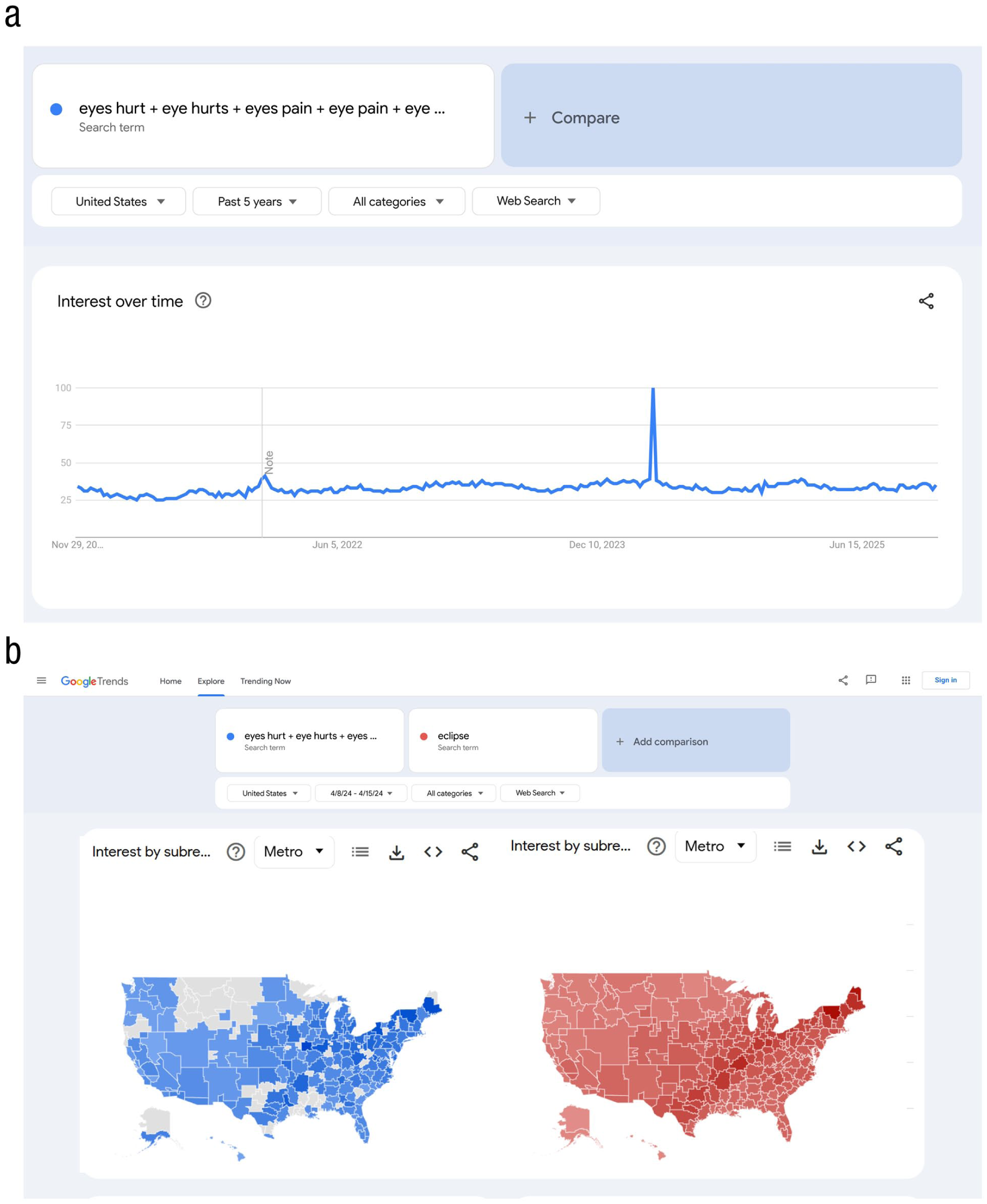
Examples of (a) interest over time and (b) interest by (sub)region on the Google Trends explorer. In Figure 1a, higher scores represent greater volume of searches related to eye pain (eyes hurt + eye hurts + eyes pain + eye pain + eye damage + eyes damage + eye symptoms). The large spike in interest corresponds to the week of the solar eclipse on April 8, 2024, when many people injured their eyes by looking directly at the eclipse (Waisberg et al., 2024). Figure 1b shows metro-level interest in the same searches related to eye pain (blue) and searches including the term eclipse (red) during the week following the eclipse. Note the close correspondence between the eclipse path and search volume related to eye pain. Darker colors represent regions with more search volume. Data are from Google Trends (www.google.com/trends).
The scores along the y-axis in Figure 1 are calculated somewhat unintuitively—they are “scaled proportions” or “proportions of proportions,” not raw counts of searches (i.e., absolute search volumes). The time point scored as 100 in any trend is the time point in the query in which relative interest was the highest—that is, the time point when the queried term was most likely to be searched for as a proportion of all Google searches in that time period. All other scores in a Google Trends query will be proportional to that score. Note that because the total raw number of Google searches varies across days, it is possible for one day to have a lower score for a given term than another even if the raw number of searches for that term is higher on that day.
We flag two cautions with how Google Trends calculates scores, which we return to later: (a) The lowest possible relative interest is represented as < 1, not 0. A time point with a zero means that there were not enough raw searches for that term to pass a prespecified privacy threshold in that time point (FAQ About Google Trends Data, 2024). (b) Scores are rounded to the nearest integer. When there is very large variation in scores, rounding can reduce precision—in the above example, if there was a day in which eyes hurt searches were 1,000 times more frequent than in the remaining 29 days, then those remaining days would all be scored as < 1, losing all the variation therein.
Daily, weekly, and monthly data
Users can specify different date ranges, and these yield different temporal granularities: daily data for queries of up to 270 days, weekly data for queries of up to 5 years, and monthly data for queries of wider time windows.
Real-time data
If users query the past hour or 4 hr, Google Trends provides by-the minute data; past-day queries yield 8-min increments, and past-week queries yield hourly increments. “Real-time” data, as these are called, come from separate cached samples of the Google database of searches than queries of older searches (FAQ About Google Trends Data, 2024). (We explain caching in the section How Reliable Are Google Trends Data?) Real-time data are not stored long-term and can be accessed only by querying the past hour/4 hr/day/week. That is, it is not possible to specify a 7-day period in the past and obtain real-time data for it—such queries will return daily scores.
With real-time data, users must consider time zones. Queries at these temporally granular scales are shown in the time zone of the user rather than those of the region(s) explored. If a user in France wants to know what time Californians are searching for Suicide (Topic), Google Trends will seem to show rises in (relative) popularity in late mornings, between 10 a.m. and 11 a.m. However, when adjusting for the time difference between France and California, it becomes clear that such searches actually rise in popularity late at night.
Linking interest-over-time scores to other data
Researchers wishing to link interest-over-time scores to other data sets must match their temporal granularities. For example, data sets with monthly data should be matched to monthly Google Trends queries. The “sample size” for interest-over-time data is simply one per time point (e.g., for weekly data, there are 52 [or 53] time points per year).
Google Trends allows users to access up to five interest-over-time trends at once—these can be different terms in the same region or the same terms in different regions 3 (or even different terms in different regions, if desired). Thus, a researcher who needs monthly data on suicide rates across states could retrieve trends for up to five states at once. On how to compare trends in more than five states at once, see the Creating Custom Data Sets section.
Cross-sectional scores: interest by region
The Google Trends explorer also displays an “interest by [region/subregion/metro/city]” panel for each term in a query. The geographical scale (and label) of this panel varies depending on the selected region. If the broadest region—“worldwide”—is selected, this panel compares interest at the level of countries; for U.S. queries, it compares all U.S. states; UK queries compare the four member-countries; for France, the subregions will be the (pre-2016) regions of France; and so on.
Interest-by-region scores are scaled in the same way as interest-over-time scores such that the region with the highest relative interest (i.e., the highest likelihood of the keyword or topic being searched across the entire specified time period) is scored as 100 and scores in other regions are proportional to it. Figure 1b displays interest by region (metro) for phrases including keywords related to eye pain (blue) and the keyword eclipse (red) in the United States during the week following the eclipse. Note that regions where the number of searches does not exceed the privacy threshold are shown in gray.
Linking interest-by-region scores to other data
Here, researchers again need to match the granularities of their data sets. The “sample size” of interest-by-region scores differs depending on the location set by the user. Setting the region to “worldwide” will yield a single region score for each country in the data set, setting the region to United States will yield a subregion score for each state (and the District of Columbia), and setting the region to a single U.S. state will yield a single score for each metro area. When searching for a single country, it is also possible to select more granular regions for that country. For example, users can query all metro areas in the United States at once.
Cross-sectional comparisons of multiple terms: compared breakdown by (sub)region
Suppose you want to compare interest in music tastes across U.S. states. Google Trends allows up to five terms at once. For example, one can compare the popularity, over a user-specified time period, of the topics Rock and roll, Hip-hop, Blues, and Pop music (see Fig. S1 in the Supplemental Material). In addition to interest over time and interest by subregion for each genre, you will find a panel titled “compared breakdown by subregion.” Here, you can see the most popular genre in each state (see Fig. 2). Darker colors represent stronger relative interest) and for each state, what percentage of searches was for each genre.

Example of the “compared breakdown by subregion” panel from a query comparing interest in four different music genres (topics)—Rock and roll, Hip-hop, Blues, Pop music—in the United States. Searches for the four genres add up to 100% in each state, as illustrated in the box with scores for Alabama. Data are from Google Trends (www.google.com/trends).
Generating and interpreting data in Google Trends
In this section, we demonstrate how to access Google-search data using Google Trends to specify which searches are included and how to interpret these data. We also evaluate the quality of Google Trends data, showing when and why some queries produce lower-quality data.
Operators in searches
Keyword queries can be customized using operators (queries including topics cannot—see below). We describe them below and summarize in Table 3. For example, a soccer fan exploring interest in the FIFA World Cup might query world cup. A space between words represents an AND command and will return all Google searches that include both the words world and cup in any order (including words in between world and cup). This soccer fan can restrict the order of the words and exclude words between world and cup using quotation marks by querying “world cup”.
Operators for Use With Keywords
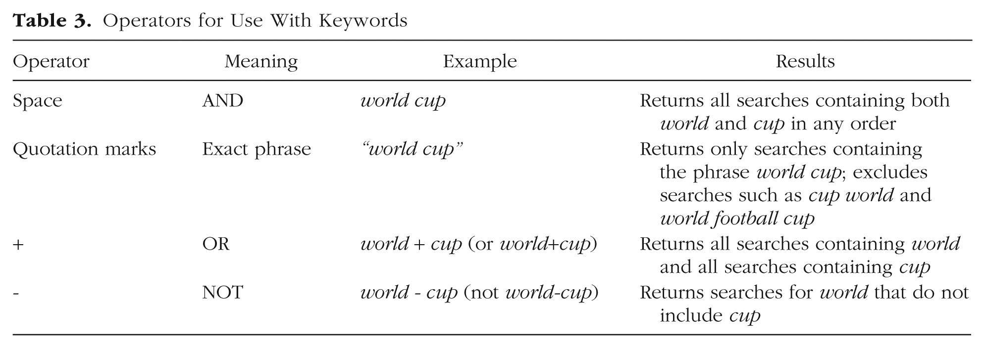
Imagine, instead, someone more interested in cups than in soccer. The popularity of the sporting tournament might make it difficult to keep tabs on cup-related trends. To remedy this, Google Trends users can exclude words using the minus sign (or hyphen): the query cup - world will give this user the desired data. (Be sure to include spaces with this operator or Google Trends will read it as a single hyphenated word.) As one would expect, cup - world does not show a spike around FIFA World Cup events, in contrast to world cup, cup world, and “world cup”.
Finally, for less selective queries, the + operator represents an OR command. Users interested in Google searches for either world or cup can query world + cup (this will include searches for the FIFA World Cup, Disney World, etc.). The + operator is especially useful for users needing to include synonyms (e.g., bunny + rabbit), plurals (e.g., bunny + bunnies), alternative spellings (e.g., color + colour), common misspellings (e.g., calendar + calender), or in applicable languages, versions of words without special characters (e.g., the French word for weather is météo, but in France, the easier to type meteo, without the accent marks, is slightly more popular; Google Trends differentiates the two versions).
Keywords versus topics
When a user types weather into the Google Trends explorer, it will make several suggestions, including weather (Search term) and Weather (Topic). 4 The former, what we call “keywords,” are queries for specific words, exactly as specified by users (including operators). 5 Keywords give the user complete control over which words are included in a query.
A topic, in contrast, is a composite of multiple Google searches related to the concept of interest. “Topics are generally considered to be more reliable for Google Trends data. They pull in the exact phrase as well as misspellings and acronyms, and cover all languages. This is more useful, particularly when looking at world data” (Basics of Google Trends, 2024).
The topics available correspond to the topic codes used in the Freebase database, which is now found in Wikidata (https://www.wikidata.org/). 6 Google Trends does not publish exactly how searches are categorized into topics; some suggest that keywords are categorized into topics by considering the links people click on after making a Google search (Woloszko, 2020). For example, if someone searches for apple and then clicks on the corporation’s website, it could be inferred that the person intended to search for the technology company rather than the fruit. Thus, this search might be categorized under the Apple (Technology Company) topic.
Topics have several benefits: (a) Topics allow users to disambiguate words that can refer to multiple constructs (e.g., apple). Fortunately, there are topics for both Apple (Technology Company) and Apple (Fruit). (b) Topics pick up on synonyms, plurals, alternative spellings, and common misspellings. By looking at the “related keywords” panel in the Google Trends explorer, users can verify that topics are related to (and presumably include) relevant words—the topic Rabbit shows the related keywords rabbit, bunny, rabbits, and bunnies; Color shows the related keywords color and colour; Calendar includes the misspelled calender. (c) Topics are claimed to be language-independent, allowing comparison of constructs globally.
Although these are impressive promises, topics often fall short of them—especially the promise of covering all languages. We review several important concerns with topics in Pitfall 4 and discuss this further in the Recommendations section.
Categories
Google Trends uses natural language processing to organize terms into categories (Arora et al., 2019). On the Google Trends explorer, users can select from a list of 1,200 categories (Woloszko, 2020), which follow a hierarchical nested structure. Users can query categories without specifying a keyword or topic (for an example, see Fig. S2 in the Supplemental Material).
As with topics, categories can be useful for disambiguating keywords that refer to multiple constructs. For example, the keyword bush will return shrub-related searches but also searches related to two former U.S. presidents. When we query for bush in the United States across the past 5 years, we get a largely cyclical pattern; when specifying the category “Politics,” however, we instead see one major spike in November 2020 (potentially because George W. Bush congratulated Joe Biden on winning the presidential election on November 8). Still, like topics, how categories are created is opaque, and it is unlikely that they perfectly filter out unrelated searches. We therefore urge caution when using categories.
Comparing interest of different terms over time
Google Trends allows users to enter up to five terms per query. When downloaded alongside other terms, trendlines are rescaled relative to each other (so except for the term with the highest relative interest, terms will be proportions of their original scores). Thus, whereas when downloaded separately each trend will have a peak of 100, when downloaded concurrently, only the trend(s) with the highest relative interest will have a score of 100. An illustration of this rescaling is shown in Figure S3 in the Supplemental Material.
Does Google Trends yield high-quality data?
In this section, we first explore the implications of “caching” by estimating the reliability of different types of searches across retrieval days. We then discuss the implications of zeros in Google Trends results and show using a simple simulation why researchers should avoid data sets with zeros.
How reliable are Google Trends data?
Google logs billions of searches daily, and many trillions have been made in the years Google has existed (Cebrián & Domenech, 2024; Rogers, 2016; FAQ About Google Trends Data, 2024). Google Trends queries are not made on this entire database of searches—this would be very computationally expensive. Rather, each day, Google Trends pulls a random sample from this database, 7 and all queries that day are made on that sample. This sample is renewed (“cached”) each day, so queries made on different retrieval days use different samples.
If Google Trends data come from new cached samples each day, how consistent (statistically reliable) are queries across retrieval days? As Cebrián and Domenech (2024) noted, previous sources have given conflicting answers: Some have suggested reliability to be high across downloads (D’Amuri & Marcucci, 2017; Stephens-Davidowitz & Varian, 2014), whereas others have reported more modest estimates (Cebrián & Domenech, 2023).
We tested whether three factors influence the reliability of Google Trends data: (a) relative search frequency (the very specific query of searches including the words I’m sad vs. the broader topic Sadness [Topic]), (b) population size (we retrieved data for the entire United States and also data for all U.S. states separately), and (c) granularity of time (daily vs. weekly data). Each of these factors can be thought of as contributing to the effective “sample size”—all else equal, there are fewer searches for unpopular (vs. popular) terms (cf. Cebrián & Domenech, 2024), in highly (vs. sparsely) populated regions (cf. Eichenauer et al., 2022), and in longer (vs. more specific) time periods. For details on this analysis, see the Supplemental Material.
As shown in Figure 3, all three factors—population size, search frequency, and temporal granularity—systematically influenced data reliability across retrieval days: Queries for the specific keywords I’m sad yield less reliable data than the broader Sadness (Topic), daily data yield less reliable data than weekly data, and queries restricted to small populations yield less reliable data than those using large populations.

Reliability estimates (intraclass correlation coefficients) of Google Trends samples across six retrieval days. On each day, we accessed data for a less common (I’m sad) and more common (Sadness [Topic]) search, at a more granular (daily) and less granular (weekly) time period, and for all U.S. states separately and the entire United States. Locally estimated scatterplot smoothing lines show trends across population size.
Are Google Trends data reliable? Yes—as long as there is a large enough search volume. The best heuristic of high reliability in Google Trends data is the lack of zeros—data sets without any zeros had excellent reliability (average intraclass correlation coefficient [ICC] = .95), whereas data sets with even up to 10% zeros had substantially poorer reliability (average ICC = .73). Data sets with more than 50% zeros—such as many of the I’m sad queries in Figure 3—yield essentially useless trends (average ICC = .06). We discuss zeros next.
Zeros are missing data: Google Trend’s privacy threshold
Why do zeros threaten reliability? At first blush, it might seem that data sets with many zeros might be especially reliable as long as those zeros appear consistently across retrieval days. However, zeros do not necessarily represent extremely low interest. Zeros represent missing data—they are displayed when the raw number of searches for a keyword or topic are below an (undisclosed) privacy threshold set by Google Trends (Cebrián & Domenech, 2023; Mavragani & Ochoa, 2019; Stephens-Davidowitz & Varian, 2014; FAQ About Google Trends Data, 2024). Trends with exceptionally low interest (but with enough search volume to exceed the privacy threshold) are displayed as “<1.”
To demonstrate how the privacy threshold functions and its implications for data quality, we simulated 1 year of Google Trends data for two terms differing in popularity (for details on this simulation, see the Supplemental Material). Results of this simulation are shown in Figure 4. These results demonstrate that when the average search interest for a term hovers around the privacy threshold, scores for that trend are often unusable, with many time points coded as zeros across retrieval days. Especially troubling is that zeros are not consistent across retrieval days. A given time point might be coded zero when accessed on one day but have a different score—even a high score—when accessed on a different day.

Results of a simulation to illustrate how the privacy threshold functions and why Google Trends data sets with zeros are unreliable. (Top) The “true” Google Trends scores as they would be calculated from samples of Popular (blue) and Unpopular (orange) searches. Each line represents a Google Trends score calculated from one of five different samples (as happens when users retrieve Google Trends data on different days). (Bottom) Results when a privacy threshold is imposed. When raw searches fall below this threshold, Google Trends returns a zero for that time point rather than the true Google Trends score. As shown in the bottom right, scores can be coded as zero inconsistently across samples (i.e., when looking at data retrieved on different days), and they can be coded as zero even if the true score is not much lower than the scores on other days.
The findings of this simulation are not just a theoretical possibility—Google Trends results often resemble the unusable Unpopular trend (Fig. 4, bottom right) from Figure 4. For example, Franzén (2023) accessed the same Google Trends query across days, reporting data that look much like this the bottom right of Figure 4, and concluded that researchers should refrain from using Google Trends altogether.
In reality, Franzén’s (2023) query—for a relatively uncommon search—simply does not have a sufficiently high search volume to consistently exceed the privacy threshold (cf. Raubenheimer, 2024). Each day Franzén repeated this query, different time points failed to exceed the privacy threshold, yielding zeros. Because the maximum peak-interest score is always coded as 100, this caused the trend to look like it has massive fluctuations when in reality, the variation in interest might have been quite small.
We echo the advice of Stephens-Davidowitz and Varian (2014) to exercise caution with data sets that include zeros. We return to this issue in the Recommendations section.
Creating Custom Data Sets
Here, we describe how to create custom data sets that extend beyond the data sets Google Trends supplies by default. The three types of custom data sets we describe all rely on the same principle: In a given trend, data points are scaled proportional to the most popular data point, so it is possible to extend default data sets by making multiple overlapping queries and harmonizing them.
We cover three types of custom data sets (see Table 4): longitudinal (extending interest over time, thereby allowing for higher temporal granularities), cross-sectional (comparing regional scores across more regions than allowed by default), and panel data (synchronizing many longitudinal trends to be on the same scale). We illustrate each with an example presented with accompanying R code.
Three Types of Custom Data Sets

Recall that Google Trends scores are rounded to the nearest integer. This has implications for users creating custom data sets. Imagine a query that yields five scores: 100, 50, 49, 2, and 1. Although rounding is less consequential for the larger scores 50 and 49 (i.e., which could be as different as 50.4 and 48.6 or as similar as 49.6 and 49.4), it substantially reduces precision for the smaller 1 and 2—the difference between their real values can range from large (0.6 vs. 2.4—the latter representing 3 times the relative interest of the former) to relatively small (1.4 vs. 1.6—in which relative interest is nearly identical).
Longitudinal data sets: interest over time at high temporal granularity
Google Trends provides daily data for interest-over-time queries of up to 270 days and weekly data for queries of up to 5 years. However, by knowing how trends are scaled, it is possible to create custom data sets that go beyond these limits. To demonstrate this, we created a trend of weekly data for Depression (Topic) in Egypt from 2011 to 2023. We downloaded three 5-year data sets of interest in Depression in Egypt, each overlapping with the next by 1 year (Trend 1 = 2011–2015, Trend 2 = 2015–2019, Trend 3 = 2019–2023). If Google Trends data were not rounded to the nearest integer, then it would be sufficient to have only a single overlapping week. We use a full year to obtain a better estimate of the ratio between the trends.
We first load these separate trends into R, calling them

We can visualize the three trends using the ggplot2 package (Wickham, 2016). This code will plot each of the lines (i.e., Trends 1–3) across time in different colors. As shown in Figure 5a, Trends 2 and 3 share a peak (on December 1, 2019), so they are already on the same scale (and thus perfectly overlap on the year they share). However, Trend 1 is on a different scale. Compare Trends 1 and 2 on the year they share—they rise and fall together (i.e., they are perfectly correlated—or would be without rounding), but Trend 1 is shifted upward compared with Trend 2.


Google searches for Depression (Topic) in Egypt, 2011–2023. We downloaded three 5-year data sets (yielding weekly data), each overlapping with the next by 1 year. Trend 1: 2011–2015, Trend 2: 2015–2019, Trend 3: 2019–2023. (a) The three trends unscaled. (b) Three trends with Trend 1 adjusted to be on the same scale as Trends 2 and 3.
Because Trends 1 and 2 are proportional to each other, we can place them on the same scale if we compute the correct scaling factor. To compute this proportion, we first create a data frame that contains only the overlapping periods: The data frame “

Next, we divide the trends by each other (which will yield data only for the weeks with values in the overlapping years) to obtain a scaling factor for each week. We then estimate the scaling factor using the code below. Rather than taking the average ratio for all weeks, we compute a weighted average, which gives more weight to higher numbers. A simulation (provided on our OSF page) shows that this generates more accurate estimates of the true ratio between trends. 8

Using this code reveals that the scaling factor between Trends 1 and 2 is approximately 0.56—that is, Trend 1 needs to be multiplied by 0.56 to be on the same scale as Trend 2. The scaling factor for Trends 2 and 3 is 1 because these two trends were already on the same scale (the overlapping time points between these two trends included the highest score). We can rescale Trend 1 by multiplying the scores in

By multiplying Trend 1 scores by this constant, we shift them downward to the same scale as Trend 2 (and Trend 3). All three trends now match (except for minor error because of rounding), although they remain in separate columns. We have named the new version of Trend 1
To create a single column with our new rescaled trend, we merge the three data frames and then take the average of the three trends, ignoring NA (missing) values. This means that the overlapping periods are the mean of the two trends—that is, 2015 scores are the average of Trend 2 and the rescaled Trend 1. Because these two trends differ only because of rounding, these changes are minimal.
First, we merge the data sets by the Week column (beginning by merging

We then calculate the average, ignoring NAs:
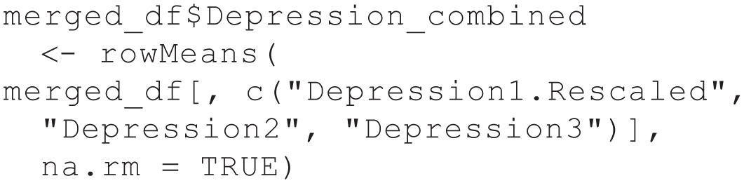
We then calculate the average, ignoring NAs:

This code creates, in the data frame
The same principles can be used to extend other longitudinal trends, such as daily data sets or sets of more than three weekly data sets. As long as researchers include overlapping periods to estimate the scaling factor, they can use these scaling techniques to create their desired data sets.
Extending cross-sectional comparisons: breakdown by (sub)region
Google Trends allows comparisons of up to five different topics/keywords in a single query. The same principles described above—download multiple and partially overlapping queries and adjust to put them on the same scale—can be used to bypass this limit.
One approach is to use the average score for each term across the user-specified time periods (these values appear at the left side of the interest-over-time panel). Holmes et al. (2022) used this approach to compare the popularity of 100 animal species (all topics). First, they found the most popular species through the process of comparison and elimination; in their list of species, this was Lion. Then, they included Lion in every query (so, four unique species plus Lion), meaning the scores for all 100 species in their data set were already set to the same scale, proportional to Lion. Finally, for each query, they saved the average score for each species, which is a rough estimate of how much interest that species garnered over time. We say “rough estimate” because the time points in a date range do not all have the same total search volume, but taking an average gives equal weight to each time point. (As an analogy, this is akin to calculating the average income in the United States by averaging the average income across all U.S. states, thereby giving them all equal weights notwithstanding differences in their population sizes.)
A more precise approach is to use breakdown-by-region scores. As shown earlier in Figure 2, breakdown by region provides percentage scores for each subregion (adding up to 100 rather than the highest interest score being scaled as 100). Because these scores are percentages, rather than the typical Google Trends scores, they require a different rescaling method.
We illustrate this approach by comparing interest in 17 different religious denominations across U.S. states. We queried Google Trends multiple times, in sets of five, for interest in all of 17 denominations. This required four separate queries. We included one denomination (LDS[Latter-day Saints]/Mormon) in every query to ensure all denominations are on the same scale. With the breakdown-by-region data, we obtain percentage scores for each state (adding up to 100) for the five denominations in each query.
The logic of the rescaling process is as follows: Suppose you have two queries (so, each with a set of four unique denominations plus LDS). In a given state, for the first set of five, LDS made up 60% of searches, and Catholic made up 30% of searches (with the other three denominations making up the remaining 10% of searches); for the second query, LDS searches made up 40%, and Baptist searches made up 20% in that state (again, with the other denominations making up the remaining searches). Remember that the number of searches for LDS in this state is equal in both queries (as long as the time frame is the same and the data are accessed on the same day). Because Catholic searches were half as common as LDS searches (60%/30%) and Baptist searches were also half as common as LDS searches (40%/20%), we can conclude that Catholic and Baptist searches were equally common in this state even though they were not downloaded in the same query. By putting them on an equal scale in this way, we can compare relative popularity of all selected denominations within each state.
To conduct this rescaling, we first read in the four separate data sets using the below code (repeat for Sets 2−4):
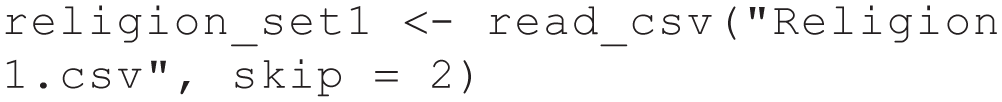
To make them easier to work with, we can also change the names of the columns. For example, we use

For each of these data sets, the set of five religions in that data set add up to 100 within each state. To put each data set on the same scale, we need to compare all religions with the same benchmark—in this case, percentage interest in the LDS Church. By multiplying each row so that interest in the LDS Church is 100, we place all denominations on the same scale across the four data sets. Table 5 shows what this process looks like in the first set before and after rescaling (showing only six of the 50 states).
Sample of Cross-Sectional Interest in Different Religious Denominations (Left) Before and (Right) After Scaling

Note: This table comes from one query of interest in five religious denominations. Only six states in the data set are shown for demonstration. Scores of < 1 were rounded to zero to be included in the analyses. LDS = Latter-day Saints.
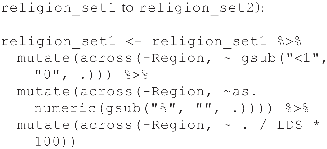
We achieved this rescaling using the below code. This code (a) changes all instances of “<1” to zero, (b) removes “%” and converts all values to numeric, and (c) divides each row by the value of the LDS column and then multiplies by 100, thus making all values proportional to an LDS score of 100 in each state. This code rescales the first data set; for the other data sets, simply substitute in the name of the data set (e.g., change
After rescaling all four data sets with the above code, we merge them:

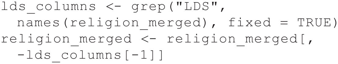
We can now remove the duplicate columns (because there was an LDS column in each data set and the value for every row in each of these columns is 100, all of these columns except one are redundant):
Finally, because of our scaling process, the data no longer represent percentages. We can convert them back to percentages by simply ensuring that the sum of each column is 100. We do this with the following code, which ensures that the sum of all numeric columns is 100:
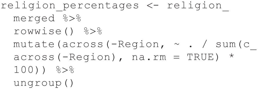
Figure 6 visualizes the relative interest in five religious denominations—Baptist religion, Catholicism, Islam, Judaism, LDS/Mormon Church. These numbers can be interpreted as percentages of all included religion searches that were for each specific denomination. For example, the score of 41 for the Catholic Church in Rhode Island means that out of all searches for all 17 denominations, 41% of the searches in that state were for the Catholic Church.
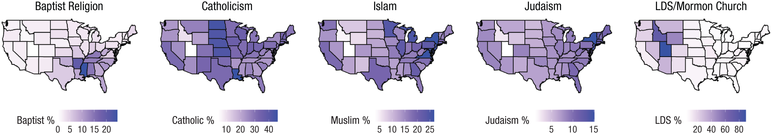
The relative popularity (in percentages) of five of the 17 religious denominations. Each map represents, for each state, the percentage of searches for the given denomination out of all 17 denominations. Darker colors reflect more interest in the denomination. Note that different denominations have different peak interests (and scales differ on the legends).
The resulting data set reflects interest in different religious affiliations across states and in some cases—as highlighted in Figure 6—also nicely tracks the distribution of actual religious affiliations. For a more sophisticated operationalization of religious activity using specific searches such as for places of worship, see Adamczyk et al. (2022).
The above example used breakdown-by-subregion scores in the United States to obtain state-level data. Users can use the same approach to compare subregions in whichever geographic location they choose. If users wish to compare such data at the country level, they can set the location to worldwide (so that the regions are countries). Because percentages add up to 100 within each region (i.e., they are not scaled to other regions), users can simply use data from the regions of interest. Because subregions are required, it is impossible to obtain such percentage data at the worldwide level.
Panel data: harmonizing interest over time across many locations
Panel data sets include longitudinal data across multiple cases (in this case, regions). Users can create panel data sets with Google Trends using the principles of rescaling presented above.
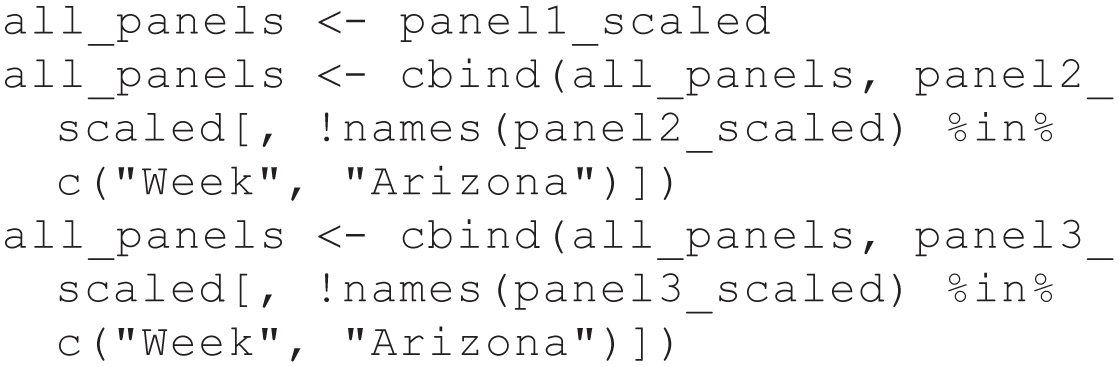
We demonstrate by creating a panel data set with trends for Abortion (Topic) across all 50 U.S. states. This required 13 queries, each with Arizona plus four additional states. By including Arizona in each query and scaling all results within each query such that the maximum score for Arizona is 100, we can create a data set with a time series for each state, all on the same scale (i.e., the Google Trends scores are comparable across states).
To do so, we first load in all 13 data sets using the below code (we provide code for the first data set only; the code for the others differs only in changing

We now have 13 data sets, each with a column called
We can do this with the following code, which multiplies all columns (except

Next, we can merge all the data frames, including only one of the Arizona columns. The below code does this by (a) creating a data frame called
We now have all of the scores on the same scale—except they are not on the original Google Trends scale, for which the maximum value is 100. To convert scores back to the original scale, we can use the following code, which finds the global maximum, computes the scaling factor to convert the maximum to 100, and then multiplies all values by that scaling factor:
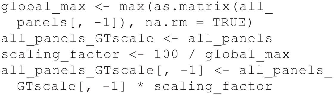
We now have a panel data set with longitudinal scores for each U.S. state’s interest in Abortion, and these scores are on the original Google Trends scale. The resulting data are visualized as a heat map in Figure 7. We have also marked several key events, and spikes in interest in abortion can be seen in response to these events: A spike in interest in Alabama during May 2019 corresponds to a bill banning abortion in Alabama. A spike across all states occurs in May 2022, and then an even larger spike occurs in August 2022. The former corresponds to the Dobbs vs. Jackson Women’s Health Organization case, which overturned the constitutional right to abortion. The decision, which was made official in June 2022, was leaked in May 2022. The latter (which was also the largest—it was scored as 100) was in Kansas in August 2022 and corresponds to a Kansas referendum on abortion legality.

Interest in Abortion (Topic) in all 50 U.S. states across time, displayed as a heat map. Tick marks along the x-axis denote key events related to abortion laws in the United States.
Note that if Arizona had the highest peak of all states (i.e., had the score of 100 been the same data point in every set of queries) or if we had instead included Kansas in every query, then no rescaling would have been necessary—all queries would have been scaled relative to the peak interest. Researchers who prefer not to rescale could first ascertain which region has the highest peak-interest score and simply include that region in every query.
Study Examples
In this section, we walk through a full analysis that could be done by linking Google Trends data to external data sets. We provide three examples: one in the main text and two in the Supplemental Material. These examples were chosen to demonstrate how different types of hypotheses can be tested using Google Trends data. In Example 1, we test the effect of a recurrent yearly event on Google-search patterns. In Example 2, we estimate the relationship between a monthly trend of Google Trends data with monthly data for unemployment in U.S. states. In Example 3, we estimate the effect of nonrecurring events on Google-search patterns.
In all three examples, we use the
One possible use of Google Trends is to estimate the effects of events, whether unique or recurring. In ongoing work, we are investigating the effects of religious fasts on well-being (Moon et al., 2026). Following Foa et al. (2022), we created composite measures of mental health and well-being using topics related to negative emotions (such that lower search volume for negative emotions indicates greater well-being). Using a small subset of this analysis, we demonstrate by examining whether searches related to Depression (Topic) are lower during Ramadan fasting periods in Egypt.
Above, we created a 13-year trend of weekly Google Trends data for Depression in Egypt. Egypt has a strong Muslim majority (about 90%), so it can be assumed that most of its inhabitants fast during the Islamic month of Ramadan. We can code which weeks of the year include Ramadan and test whether depression-related searches decline in Egypt during those weeks.
First, we create a vector with weeks coded as Ramadan. We selected weeks with at least 4 days of Ramadan (i.e., majority-Ramadan weeks):

Next, we create a dummy-coded Ramadan variable for the 13-year weekly trend we created earlier (

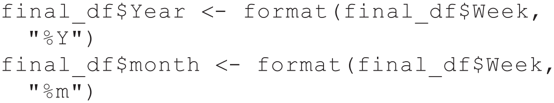
Next, we create variables indicating the year and month (to control for year-by-year and seasonal fluctuations in depression-related searches):
Finally, we run a fixed-effects model using the fixest package. This fixed-effects regression controls for year-to-year differences in searches and accounts for normal seasonal variation in searches (by controlling for month). We also cluster standard errors by year because weekly observations within the same year are likely correlated:

We found that depression-related searches are significantly lower during Ramadan (vs. non-Ramadan periods) in Egypt, b = −4.53, SE = 1.08, t = −4.19, p = .001.
This basic analysis can be scaled up. In the full study (Moon et al., 2026), we included all countries that (a) had sufficient data (i.e., data sets without zeros—see Recommendations) and (b) have populations that are at least 75% Muslim. We also used a wider range of topics (Depression, Sadness, Antidepressant, Psychological Stress, Apathy) to create composite measures of well-being and test robustness of the effects.
Potential Pitfalls in Google Trends Data
As with any tool, researchers need to understand how to use Google Trends responsibly. We overview common pitfalls researchers should be aware of.
Pitfall 1: data quality is not guaranteed
Google’s search algorithms are constantly being updated to improve service to clients and users, and these changes likely influence Google Trends data in ways unpredictable to users (Lazer et al., 2014). Some major changes that might influence Google Trends data are marked in the Google Trends explorer (e.g., at the start of 2011, 2016, 2017, and 2022). However, the specifics of these changes are not publicized.
This means that the data quality can change over time—some changes might improve the quality of data along the availability within the range of dates offered by Google Trends (e.g., the data seem to have improved after some of the above algorithm shifts). Some changes might also affect prior data. For example, Algan et al. (2019) found large jumps in several searches (e.g., pregnancy) at the beginning of 2011 (following a major, marked algorithm change); however, when we tried to replicate those queries, we no longer saw those jumps, suggesting that more recent algorithm changes have altered previous data.
In addition, we have occasionally noticed patterns that seemed highly implausible. For example, on November 6, 2023, we noticed that on October 30, 2023, there were worldwide anomalies on nearly every term we examined—some spiked, and others dipped to near < 1 (see Fig. S4 in the Supplemental Material). When we repeated these queries on subsequent days, these anomalies disappeared, suggesting that they represented a quirk in Google Trends rather than drastic and hard-to-explain shifts in worldwide internet-search behavior. Our advice for researchers noticing such aberrant patterns is to check whether they disappear when the data are accessed on subsequent days and if they do not, to avoid using data with such patterns.
In sum, researchers using Google Trends cannot audit the specific ways in which Google Trends data are collected, aggregated, or geographically assigned. For example, assignment of searches to topics and geographic assignment (e.g., for individuals near borders or those using VPN services) may be imperfect. Google Trends was not created specifically for researchers and does not make guarantees about data quality. Although we suspect and hope that the quality of Google Trends data will improve over time, this is not a certainty.
Pitfall 2: Google-search data are highly representative but not fully
In many countries, an examination of Google-search data seems to suggest that interest in science has declined over the last 20 years. However, as Stephens-Davidowitz and Varian (2014) suggested, an alternative possibility is that the demographics of Google users—in the United States and likely elsewhere—has changed: Early adopters tended to be more computer-literate and more interested in science and technology than the average person (Mellon, 2013). Thus, it might not be that general interest in science declined but that people who are less interested in science have gained more access to the internet. (It is also the case that the menu of offerings available on the internet has increased over time.)
Although nowadays nearly the entire U.S. population uses Google, this is not the case for developing countries (or countries where Google is not the search engine of choice, such as China and Russia, where Baidu and Yanex, respectively, are more popular). Thus, researchers should be aware that Google-search data may not be representative of the entire world population across both time and geographical regions.
Another reason Google-search data may not be representative stems from what people use Google for. There may be different rates of technology use by cultural background or socioeconomic status (Pew Research Center, 2021). In addition, different populations might vary in how they use Google—it could be the case that search behavior is a valid indicator of some underlying psychological train in one population but not in another.
In sum, although Google handles most of the world’s internet searches, it is not a random and fully representative sample of the world’s population (although it is likely more representative than traditional research methods, such as surveys on university undergraduates or samples recruited through crowdsourcing platforms, such as Amazon’s Mechanical Turk and Prolific Academic). Around the globe, there are still wide swaths of people without stable internet access, and even among internet users, not all people use Google in the same way.
Pitfall 3: construct validity can be difficult to establish
Google Flu Trends showed much early promise, as we described above, but it has become a cautionary tale about using big data for prediction (Lazer et al., 2014). The accuracy of the predictive model declined over time, especially during the H1B1 (swine flu) outbreak in 2013. In part, this decline in accuracy stemmed from one potential pitfall with Google-search data: People might make the same Google search but for very different reasons. During the H1B1 outbreak, news of the flu spread fast; many people became worried and curious about this new flu variant and searched for H1B1 symptoms without being sick (see Milinovich et al., 2014). 9
The case of Google Flu Trends underscores the fact that construct validity—whether Google Trends scores are an appropriate proxy for the construct of interest—can be difficult to establish and might even change over time. The link between a search and a construct is more straightforward the fewer inferential steps a researcher takes—it seems reasonable to infer that people searching for wordle answer and today wordle want to know the daily answer to the popular New York Times brainteaser (Wormley & Cohen, 2023). However, it is less clear whether such searches are indicators of constructs that are multiple inferential steps away, such as being more likely to be a cheater in general. The more inferentially removed a construct is from the search(es) that proxies it, the more caution is required.
Thus, researchers must consider trade-offs between query specificity and construct validity. In many cases, it is possible to construct queries with very high face validity for some variable of interest. For example, searches for anti-Black epithets work especially well as a proxy for racism because they are so taboo that it is difficult to imagine using them without harboring some level of prejudice. Likewise, comparing frequencies of son gifted versus daughter gifted seems like a straightforward way to assess how readily people look for talents in boys versus girls (Stephens-Davidowitz, 2017). However, such specific queries may not yield sufficient data. For example, there are fewer people who search “I want to kill myself” than there are that search for suicide. Although the former has higher face validity, the latter is more likely to yield usable data (especially with more temporal or geographical granularity). (See Fig. 3, where we show this with queries for I’m sad vs. Sadness [Topic].)
Furthermore, as mentioned under Pitfall 2, people likely use Google in different ways. Thus, even if a query serves as a valid proxy in one geographical location or at one point in time, this may not generalize. (See also our discussion of topics in Pitfall 4.)
Exogenous factors and fluctuations in construct validity
Foa et al. (2022) found that in the UK, Boredom (Topic) searches closely tracked reported boredom from YouGov surveys (r = .85). When attempting to replicate these analyses with more recent dates, we noticed a spike—more than 10 SD above the mean—in relative interest in Boredom (Topic) on June 5, 2023 (see Fig. S5 in the Supplemental Material). Upon closer inspection, the top related search on that day was “ennui,” and more revealing, the related search showing the highest rise in popularity on that day was ennui wordle—it was the answer to The New York Times Wordle puzzle that day. That is, this spike in Google searches was simply due to an exogenous influence rather than a real increase in boredom.
In contrast, there was another large (but less extreme) spike in the popularity of Boredom (Topic) in March 2020. This spike corresponded to the first UK COVID-19 lockdown, and related searches in this period include bored during lockdown; this spike, therefore, seems to represent an actual increase in boredom.
Although both events represent spikes and both can be attributed to exogenous factors (either the Worldle answer of the day or a government-imposed lockdown), we would consider only the latter to represent a genuine shift in felt boredom. (Consistent with this, YouGov data also show a spike in self-reported boredom during this time.) Without YouGov survey data for comparison, one tool to determine which spikes are “genuine” are the related keywords/topics—for large spikes, these can provide clues to alternative reasons why a keyword or topic are being searched. Users will need to use their best judgment to determine which patterns they treat as genuine.
Google trends data are not individual-level data
Google Trends data are society-level data. That is, they represent the search behavior of the population specified in the query. Note that correlations between variables at the individual level are not always the same as correlations at the society level—a phenomenon known as “ecological correlations” (Robinson, 1950), or the “ecological fallacy.”
For example, consider the example we began this article with, whereby more racist counties in the United States (i.e., counties where people made more searches for anti-Black racial slurs) had lower vote shares for Barrack Obama in the 2008 U.S. presidential election than expected relative to previous elections (Stephens-Davidowitz, 2014). Although it is tempting to conclude that racist individuals were less likely to vote for Obama, one cannot conclude this with absolute certainty, only that racist counties were less likely to vote for Obama. In addition, aggregate-level correlations obscure important within-groups variability—for instance, a county-level correlation between search terms and voting patterns does not necessarily tell much about the distribution of these behaviors within counties.
What does this mean for users? First, users should use precise language about the levels of analysis in their claims (e.g., “counties with more racist searches” or even “racist counties” rather than “racist people”). Second, when possible, users can triangulate Google Trends findings with additional evidence. A study that establishes an effect using individual-level data and then conceptually replicates that effect (perhaps in different regions or across time) using Google Trends would be especially compelling. When such triangulation is not possible, it is important to acknowledge this limitation explicitly.
Finally, it is important to consider potential confounding factors that might create spurious society-level correlations. For instance, shared demographic, economic, or other cultural factors might influence both search behavior and the outcome (or predictor) of interest.
Effect-size considerations
We have suggested several threats to construct validity above; however, whereas some of these threats (e.g., large spikes) are easily detected and accounted for, there are subtler threats that are less easy to detect: small or gradual changes in the demographic composition of a region, evolution in how words are used, or shifts in how Google Trends calculates topics. These subtle factors can add up, making Google Trends data noisy.
In our view, one implication of this is that users should be particularly cautious with research questions that deal with small effect sizes. Even in the best-case scenario, Google Trends proxies are not precise indicators of psychological constructs but include measurement error. Because of the possibility of substantial noise, researchers likely need a relatively large signal (or effect size) to cut through it.
Pitfall 4: issues with topics
Topics have some impressive benefits. Yet there are several reasons to use them with caution. First, Google Trends does not report how they are created. Although related keywords/topics can be useful checks of the constructs that are associated with (and potentially included in) a topic, users cannot uncover the full list of constructs that make up a topic or the precise manner in which they are combined. Thus, both quality control and making specific inferences are more difficult with topics than keywords.
Second, although they supposedly “cover all languages” (Basics of Google Trends, 2024), topics do not include terms from all languages equally (Arora et al., 2019; Woloszko, 2020). Consider Weather (Topic). In the United States, when we compare queries for Weather (Topic) and the weather keyword, they return nearly identical relative search volumes (suggesting that in English-speaking countries this topic is almost exclusively based on the keyword weather). Elsewhere, as expected, Weather (Topic) tracks the words people use in local languages to search for the weather forecast—météo in France, ריווא גזמ in Israel, and so on.
However, at the time of this writing, Weather (Topic) does not seem to include the Spanish words for weather (tiempo or clima). When we queried Weather (Topic) worldwide, interest-by-region scores were missing (i.e., zeros) for all Spanish-speaking countries except for Spain. Looking at the related keywords within Spanish-speaking countries, the Spanish words for weather were not listed; Spain’s present but low score seemed to be driven by sufficient search volume for the English and Catalan terms.
Thus, queries for Weather (Topic) might erroneously lead one to conclude that Spanish-speaking countries are not interested in the weather. Other topics lack coverage in other languages (Woloszko, 2020). Thus, when using topics, users should explore the associated topics and keywords in each of the languages of their regions of interest to make sure that the topic is valid in that language and region and across the entire selected date range.
Third, although topics are supposed to isolate constructs of interest (e.g., differentiating Apple [Fruit] from Apple [Technology Company]), they sometimes fall short. Consider the example of Holmes et al. (2022), discussed above, who compared interest in 100 animal species. Holmes and colleagues concluded that Lion was the most popular animal topic. However, when replicating their analysis, we noticed a spike for Lion on July 21, 2011 (Fig. S6 in the Supplemental Material). Upon closer inspection, the top related search keywords (after lion itself) on that day were os lion and lion mac—the new operating system for Mac computers released the day before.
When we limit the Lion (Animal) query to the range of dates before the new Mac operating system was released (2004–June 2011, in contrast to Holmes et al., 2022, who looked at 2004–2020), we find that it was Tiger (Animal), not Lion (Animal), that was most popular. 10
Fourth, we have sometimes observed inexplicable shifts in some topic scores. For example, the topic Psychological Stress (Illness) is a decent proxy for self-reported stress (Foa et al., 2022). However, this topic inexplicably dips around the end of 2016, recovering toward the end of 2018, worldwide. The query stress + stressed does not show a similar dip, suggesting this dip might be a quirk of the topic rather than a broad mental-health shift during this time period (see Fig. S8 in the Supplemental Material). The cause of this dip is not obvious to us, and we can only recommend that Psychological Stress (Illness) be used with caution during this time period.
Recommendations
We close with recommendations for the responsible use of Google Trends, including choosing appropriate data, best practices to safeguard data quality, and recommendations for open science and transparent reporting.
Recommendation 1: creating proxies for psychological variables
Perhaps the most straightforward use of Google Trends—in terms of face validity, or the small inferential gap between Google-search data and constructs—is to explore how much information people seek about different constructs, including because of how salient different constructs are (what political scientists term “issue salience”). For example, political scientists have explored interest in corruption, world trade, or human rights (Ajzenman, 2021; Dancy & Fariss, 2024; Mellon, 2013, 2014; Pelc, 2013). With such uses, it does not require a large inferential leap to conclude that people in countries with, for example, high search volumes for human rights are currently thinking more about human rights.
However, psychologists often want to go beyond such simple (and face valid) uses, to explore constructs such as thoughts, feelings, and behaviors. Google-search data are more valuable to the extent that they can be used as proxies for such constructs. As noted earlier, it is possible to create proxies for many psychological constructs (see the examples in Table 1), but doing so takes some additional care—and creativity. We have four recommendations for researchers building proxy variables.
Do not overlook face-valid terms
In our opinion, some of the most interesting uses of Google-search data rely on face-valid queries—it stands to reason that people who search for taboo racist slurs or phrases containing the words how to suicide harbor at least some racism or have at least some suicidal ideations, respectively. If you can find a face-valid keyword(s) or topic with a sufficiently high search volume, that is likely an excellent choice.
Consider the point of view of Google users
People often turn to Google to solve problems. Considering the types of problems or needs people have and the searches they are likely to type into Google to solve these problems or fulfill those needs can suggest reasonable proxies. For instance, social and clinical psychologists might want proxies for constructs related to mental health and well-being, such as happiness. Google Trends has a Happiness topic. However, it is not clear that people who are happy are more likely to search for happiness-related words (indeed, Happiness [Topic] seems to be more closely related to Birthday [Topic] and happy birthday).
A more valid proxy might be the inverse of happiness—Sadness (Topic) or even Depression (Mood) or the concrete solutions people who are sad might seek, such as antidepressants or therapists near me. In contrast to happiness, when people have issues, such as a lack of happiness, it does seem that they are more likely to turn to Google for information or advice.
Consistent with this notion, previous research has found that searches for negative—not positive—emotions are more predictive of well-being. Foa et al. (2022) showed that searches for most negative-emotion topics (e.g., Sadness, Boredom) are adequate proxies for these emotions (i.e., Google Trends scores for these negative-emotion topics closely tracked these self-reported emotions in YouGov surveys); none of the positive-emotion topics (e.g., Happiness or Optimism) were adequate proxies. Likewise, Greyling and Rossouw (2025) used machine learning to test which Google Trends searches are most closely related to survey data on subjective well-being and found that “sad,” “headache,” and “depressed” were the three most important queries.
To summarize, when constructing a proxy, it is helpful to think not about the topics/keywords that describe the construct of interest but about what kind of information this construct will prompt people to seek. In many cases, it might also be useful to consider the opposite of the construct of interest: What information do people seek when severely lacking the construct of interest?
Consider creating composite indices
Many of the uses of Google Trends shown in Table 1 incorporate several keywords or topics to create composite scores or indices of a given construct. For example, Foa et al. (2022) created a measure of well-being that incorporated several negative-emotion topics. Adamczyk et al. (2022) created cross-cultural religiosity scores by using several queries related to religiosity.
One strength of these indices is that they apply appropriate weighting to multiple keywords or topics. This means that these indices are less susceptible to idiosyncratic shifts in a single variable. For example, an exogenous influence that causes a large spike in a single keyword will be less consequential if that keyword is one of several in a composite measure.
Validate proxies when possible
Ideally, users will be able to validate their proxies by showing that they correlate with more standard indices of the underlying construct. For example, Foa et al. (2022) created a measure of well-being using negative-emotion topics such as Sadness and showed that in the UK, weekly searches for these negative emotions correlate highly with weekly YouGov survey data. The correlations between temporal fluctuations in the self-reported emotions and Google searches related to these emotions suggested that searches are at least somewhat indicative of the actual experience of these emotions. To avoid overfitting, Foa et al. also ensured that their measure was similarly predictive in an “out-of-sample” period.
When such validation data are not available, researchers might validate their proxies by checking whether they correlate with variables that are known to strongly vary with the underlying construct. For example, happiness—and its proxies—might rise on holidays such as Christmas in countries that celebrate it (one of the happiest days of the year; Stephens-Davidowitz, 2017), and proxies for religiosity should predict outcomes typically associated with religiosity (Adamczyk et al., 2022).
Recommendation 2: safeguarding data quality
Aim for data sets without zeros
We recommend avoiding data sets with zeros whenever possible. As shown above, data sets without zeros typically have high reliability across downloads (average ICC = .95, minimum ICC = .82). Although the minimum ICC of .82 represents good reliability, researchers who conduct analyses in which even modest measurement error is problematic (e.g., testing small effect sizes) may wish to download the relevant data multiple times to verify that the ICC is higher than this minimum or if it is not, to average scores across downloads. (However, we reiterate our caution that Google Trends is inherently a noisy data source and thus not likely well suited to detect small effects.) In general, for most applications, a single download of a data set will be sufficient as long as it does not contain zeros.
What to do if there are zeros
Option 1: adjust your query
If your data have zeros, the most ideal solution is to adjust the query so that scores more consistently rise above the privacy threshold. We describe adjustments that can help.
Find keywords or topics with higher search volume
One way to increase the search volume of a query is to find more popular keywords or topics, such as a synonym or a related term. With keywords, you could use the + operator to make the query broader (e.g., if rabbit is too rare a search, one could change the query to rabbit + rabbits + bunny + bunnies, which might more reliably surpass the privacy threshold). As mentioned above, there is a trade-off between the specificity of a query and the likelihood that it will yield consistent data.
Reconsider your temporal and geographical granularities
As shown earlier, more granular queries yield less consistent results (and are more likely to yield zeros). If an interest-over-time trend includes zeros, consider using weekly (instead of daily) or monthly (instead of weekly) data (do this simply by making the query cover a longer period even if the entire period is not needed); if subregions yield inconsistent data, consider zooming out to the country level.
Consider your time period
Older Google Trends data (2004–2008) tend to be more variable and are also likelier to contain zeroes (Raubenheimer, 2024). In part, this may be due to fewer people using Google during that period (i.e., a smaller sample size). When older data are not necessary, we suggest 2011 as a sensible starting point for collecting higher-quality data. If earlier data are necessary, be aware that those periods may be somewhat more variable.
Option 2: consider accessing the data across multiple retrieval days
If changing the search terms or reducing the query granularity does not eliminate zeros or is not feasible for your research question, consider downloading the data multiple times and combining the downloads.
If there are a few zeros throughout a trend on one retrieval day, it is possible that those periods will have nonzero data on subsequent retrieval days. After accessing the data on multiple retrieval days, you can average together all of the nonzero scores (or take the median; Raubenheimer, 2024). The amount of downloads needed will vary depending on the nature of the data—if there are a small amount of zeros, only a few downloads will likely suffice.
Note that if your query contains many zeroes, it is likely not possible to obtain quality data (cf. Raubenheimer, 2024).
What to do if you need to deal with zeros
If you cannot avoid using data sets with zeros, we recommend coding zeros as missing because they do not necessarily represent extremely low interest. We recommend extreme caution when using data sets with zeros. Furthermore, even with zeros coded as missing, the rest of the data are likely to have greater measurement error than data sets without zeros.
Other threats to data quality
Rounding
As noted earlier, Google Trends rounds scores to the nearest integer. Although this is not a problem with large numbers, it can drastically reduce precision when working with small numbers. As an extreme example, imagine a trend such as Depression that has a small fraction (e.g., < 1%) of as much research volume as a trend such as Weather. In such cases, if the two trends are downloaded together, then all (or nearly all) of the less popular trend scores will be rounded to 1 (or “< 1”). To avoid removing all variation in the less popular trend scores, it would be necessary to download the two trends separately.
However, rounding can also reduce precision within a single trend if one time point has exponentially more search volume than other time points. In this case, one solution would be to download data for the desired time periods around the large spike. For example, suppose a trend is composed of weekly scores below 10 with only a single large spike at 100. To obtain greater precision within the non-100 weeks, you could download weekly data spanning up until just before the week coded as 100 and again for all the weeks following that week. Although this would put the before and after weeks on different scales, it would make rounding less consequential; researchers could then harmonize the two sets using the principles discussed in the Creating Custom Data Sets section.
Outliers
We suggest checking for outliers by both visually examining the trendline and mathematically searching for values high above or below the mean (we avoid making specific recommendations about outlier cutoffs). This is particularly important if your analysis relies on a single trend (rather than a composite, in which a single aberration would be less influential).
Outliers can threaten the quality of the data in at least two ways. First, they might represent threats to construct validity. As discussed above, one example of this was searches for Boredom (Topic) peaking because the Wordle puzzle of the day was ennui. To inspect spikes, we recommend zooming in on the affected period (e.g., the week when the spike occurs) and examining related keywords and topics (both top and rising). In this case, we found related keywords that included wordle, leading us to verify the Wordle answer for that day and to conclude that this spike does not represent a genuine increase in boredom.
Researchers must then decide what to do with spikes that seem to stem from unrelated events—in some cases, this spike is short-lived and could be reasonably coded as missing or imputed using standard approaches to missing data. In other cases, such as the Lion case discussed earlier, there seemed to be sustained interest in lion os—considering this, there is perhaps no straightforward way to salvage these search periods.
Second, even “true” outliers can pose a problem by making the data less precise—see the discussion of rounding above.
Algorithm updates
As described above (Pitfall 1), Google Trends notes several improvements to its algorithm (e.g., to its geographical assignment in 2011 and to its data-collection system in 2016, 2017, and 2022). In some cases, there might be some shifts in the data quality following these periods.
If researchers spot such anomalies following improvement time points, they might consider correcting for them by either adjusting the data (Algan et al., 2019) or adding a dummy code for before/after the time points. Whether an adjustment is necessary (and what the correct adjustment should be) will depend on the nature of the data set and the intended analyses.
Recommendation 3: best practices in open science and reporting
Preregistration
Preregistration with Google Trends is less straightforward than with most studies using primary data. Unless researchers make predictions about future events (e.g., a hypothesis about how an upcoming holiday will alter search behavior), then preregistration will not precede the creation of the data.
Nevertheless, it can still be useful to preregister secondary data analysis (Weston et al., 2019). We recommend preregistering a research plan, including (a) the exact keywords or topics to be used, (b) the geographic scope, (c) the temporal scope (e.g., whether daily or weekly data will be used and across what range), and (d) the full analysis plan.
Of course, researchers who preregister their plan before accessing the data cannot be sure that the data they plan to use will be high quality. Thus, we recommend preregistering decision rules, such as what you will do if a data set has zeros and how you will treat outliers. For example, you might preregister an analysis using daily data but specify that if these data sets include zeros, then you will use weekly data instead. You might also specify contingency plans in the search terms or keywords you will use (e.g., “We will examine whether searches for ‘I’m sad’ decline over time, but if this trend includes zeros, then we will instead examine the topic Sadness.”)
Reporting
To minimize ambiguity, always specify the exact queries used. When described, it should be clear whether a query used keywords or topics and with keywords, whether any operators (e.g., quotation marks) were used. We introduced and followed throughout this article several conventions described in Table 2 (e.g., italicizing queries).
Always specify the exact range of dates, temporal granularity, and geographical regions queried. When reporting cross-sectional (interest by region) scores, it may seem that the date range is unimportant, but terms that are more popular during one time period are not necessarily popular during all time periods.
We recommend including Google Trends links (for downloads from the explorer) or code (if downloaded using the API or a pseudo-API) showing exact downloads (which would include the exact range of dates and geographical region). Results will not replicate exactly (because of daily cached samples), but for downloads of trends with high enough search volume, these differences will be negligible.
Conclusion
Google-search data are a potential gold mine, holding promise for tackling many psychological and social scientific research questions. Google Trends is a free, easy-to-use, and highly adaptable tool; it makes available both longitudinal and cross-regional data across much of the internet-using world; data are available nearly immediately and can range from real-time (by-the-minute) data to monthly data going back years; it circumvents many of the shortcomings of traditional research methods (e.g., desirability biases); it reaches people at times and places for which traditional methods are unlikely to reach them; and it is highly amenable to taking advantage of natural experiments and sophisticated research designs that are underused in psychology.
Nevertheless, Google Trends data can be messy. Without proper care, it is easy to download data sets full of low-quality data; researchers are unable to audit the algorithms that generate the scores they download, and these data may sometimes be unreliable or invalid; Google Trends relies on users of Google’s search engine, which may not be representative of the entire population; it is sometimes difficult to establish construct validity, and construct validity can be compromised by changes across time or by exogenous events; and topics—which are offered as a language-independent alternative to keywords—frequently fall short of their promised function. We hope this tutorial will provide the knowledge necessary to exercise sufficient caution to understand and make use of this tool.
Supplemental Material
sj-docx-1-amp-10.1177_25152459251409146 – Supplemental material for Google-Search Data for Psychological Scientists: A Tutorial and Best Practices
Supplemental material, sj-docx-1-amp-10.1177_25152459251409146 for Google-Search Data for Psychological Scientists: A Tutorial and Best Practices by Jordan W. Moon and Michael Barlev in Advances in Methods and Practices in Psychological Science
Footnotes
Acknowledgements
This article does not involve human participants, personal data, or experimental procedures requiring ethical approval. All data included are publicly available, and no identifiable individual information is used.
Transparency
Action Editor: Pamela Davis-Kean
Editor: David A. Sbarra
Author Contributions