
Abstract

The use of survival methods
Imagine we are studying a population of individuals undergoing a particular type of surgery and we wish to estimate the average survival time. If we can follow all study participants until their date of death, then we could use a standard approach (i.e. mean or median) to calculate this average. Furthermore, if we wished to compare average survival times for different surgical methods, we could use hypothesis tests such as t-tests or their non-parametric equivalents. However, several situations exist in which we do not observe the death of all study participants; we only know they were still alive a certain time after their surgery (e.g. date of loss to follow-up or study end). We say that individuals were censored on this date. 1
How do we account for these censored individuals? One possible approach would be to calculate the average survival time among those who died. Here we are likely to be underestimating the average survival time; individuals who survived for a shorter time period are more likely to be included in the calculation. 1
Similarly, we may wish to calculate the percentage of our study participants who are still alive at a certain point in time (say 5 years post-surgery). If we know whether all individuals are alive or dead at five years, then we can easily calculate this percentage. However, if some individuals do not have five years' follow-up available (i.e. they are censored before 5 years) then this is not so straightforward. We must use survival analysis techniques that take account of this censoring in both situations described here.
Kaplan–Meier methods
A commonly used approach to account for censored data was developed by Kaplan and Meier. 2 Lets look at how this method is applied using a hypothetical example. We have studied 100 individuals following a particular type of surgery and are interested in the median time to death and the percentage still alive at five years. As individuals were recruited to the study at different times, not all individuals have a full five years' follow-up available. However, we have recorded the time from surgery to date of death of all individuals who died and also the length of available follow-up for those who were alive at the end of the study period. This is sufficient information to enable us to use Kaplan–Meier analysis techniques, available in most computing statistical packages. The results of this hypothetical study are shown in a Kaplan–Meier plot in Figure 1.
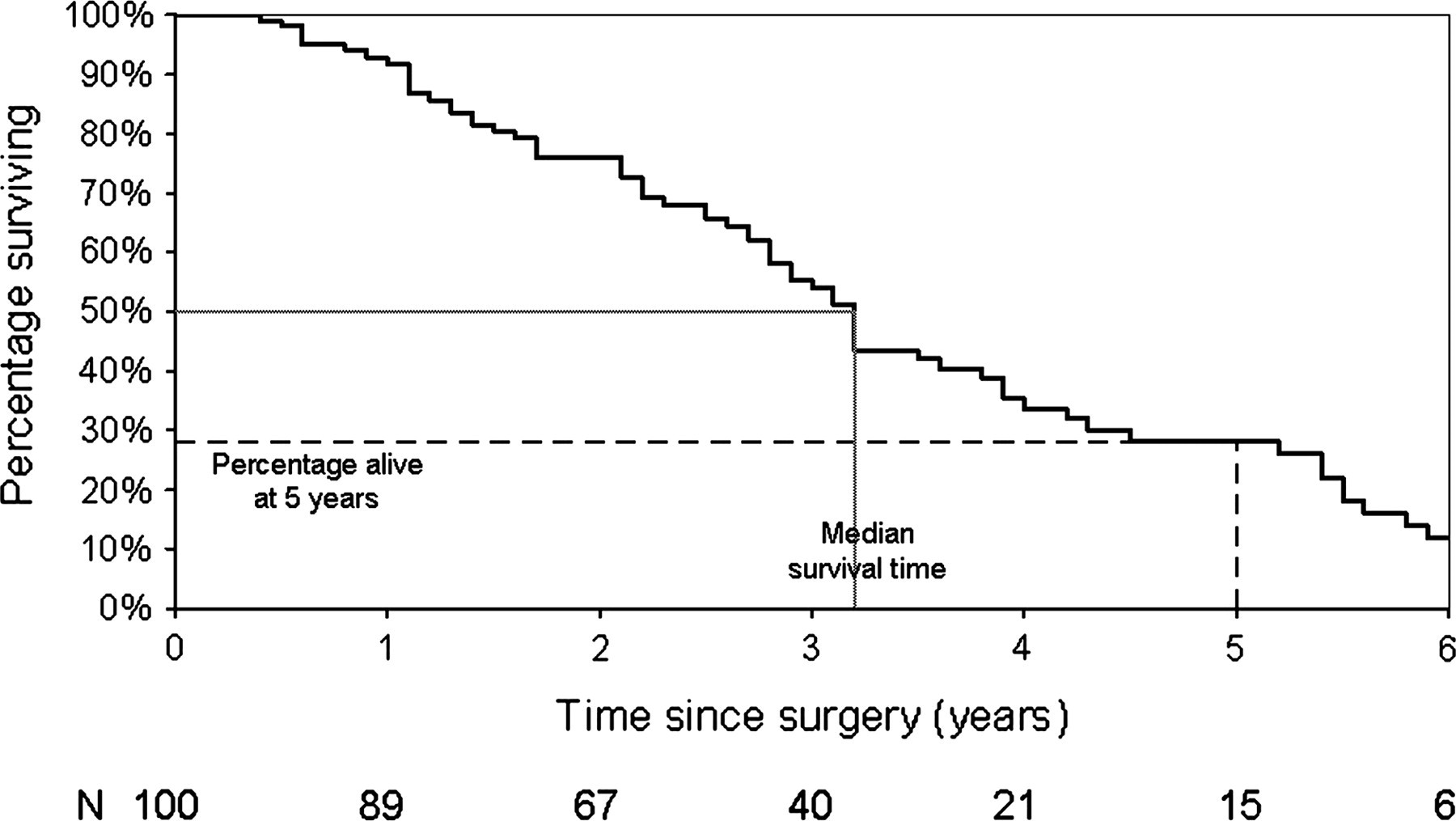
Kaplan–Meier plot of time to death among individuals receiving a particular type of surgery. Hypothetical data-set of 100 individuals
This plot shows the proportion still alive over the study follow-up period, after accounting for censoring. Kaplan–Meier plots have a ‘stepped’ appearance, with each step representing a time at which a death occurred. 3 Note that we can equivalently plot the percentage that died over the follow-up period (so the graph would start at 0% and ‘goes up’ rather than starting at 100% and ‘going down’).
Using this plot, we can calculate the median survival time (i.e. the time at which 50% of the cohort are still alive). This is marked in Figure 1 by a dotted line. We can see that a value of 50% on the y-axis corresponds to a value of 3.2 years on the x-axis. Therefore, we estimate that the median (average) survival time post-surgery is 3.2 years. This Kaplan–Meier approach also enables us to calculate a 95% confidence interval (CI) for this value, which again can be calculated using most computing statistical packages using Greenwood's method. 3 In our example, the 95% CI is 2.8–3.8 years. Note that this is not the same value as if we calculated the median survival time among those who died, which is 2.7 years.
Similarly, we can use the Kaplan–Meier plot to calculate the percentage of individuals who survive to five years postsurgery. This is marked in Figure 1 by a dashed line. We can see that a value of five years on the x-axis corresponds to a value of 28% years on the y-axis. Therefore, we estimate that 28.1% of individuals will survive to five years post-surgery. A statistical package tells us that the corresponding 95% CI is 17.3–39.0%.
Bland and Altman 3 list three assumptions that are made when carrying out a Kaplan Meier analysis such as this. Firstly, those who are censored had the same probability of death as those who remained in the study. Secondly, we assume that the probability of surviving is the same for all individuals recruited to the study, regardless of whether this was at an early or late point in the recruitment period. Thirdly we assume that we know the exact date at which death occurred.
There is insufficient space here to provide detailed advice on presenting Kaplan–Meier plots and there are already several good references that fulfil this role. 3–7 However, it is worth noting two factors in particular. Firstly, it is helpful to provide the number still at risk (i.e. the number still under follow-up) at various time points as a footnote to a Kaplan–Meier plot, as in Figure 1. Secondly, the y-axis should be scaled from 0% to 100% so that readers are not misled as to the frequency of the event being studied.
Example
We have until now been considering time to death as our outcome. Despite being commonly known as survival analyses, these methods can clearly be used for outcomes other than death. In the June 2010 issue of Phlebology, van Groenendael and colleagues compared conventional surgery and endovenous laser ablation of recurrent varicose veins of the small sapphenous vein in a retrospective study. 8 One outcome of the study considered was time to recurrence. The authors used a Kaplan–Meier approach to assess this and found similar recurrence rates under the two interventions.
Summary and further survival method techniques
In situations in which censored data are present, the Kaplan–Meier method is a useful technique. Formal methods for comparing two or more curves can be performed using the log-rank test. 9 Furthermore, multivariable analyses can be performed using Cox Proportional Hazards models. 10