
Abstract

Introduction
In the previous issue of Phlebology, we considered how the accuracy of a diagnostic test can be assessed by calculating its sensitivity and specificity. 1 We also noted that, although sensitivity and specificity are very useful to define the accuracy of a test, they may not provide us with all the information that we require in a clinical situation. When a patient obtains a test result, we most likely wish to understand the implications for that particular patient; i.e. how likely is it that they have the disease in question. If we only know the sensitivity and specificity of a test, we are unable to directly answer this question without further calculation.
Calculation of positive predictive value and negative predictive value for hypothetical example
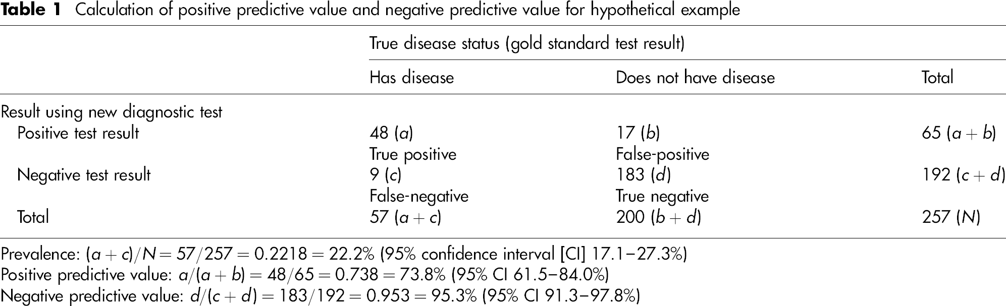
Prevalence: (a + c)/N = 57/257 = 0.2218 = 22.2% (95% confidence interval [CI] 17.1–27.3%)
Positive predictive value: a/(a + b) = 48/65 = 0.738 = 73.8% (95% CI 61.5–84.0%)
Negative predictive value: d/(c + d) = 183/192 = 0.953 = 95.3% (95% CI 91.3–97.8%)
Positive predictive value
The positive predictive value (PPV) of a test is defined as the proportion of those with a positive test result who truly had the disease (i.e. were correctly diagnosed). 2 In our study, 48 individuals out of the 65 individuals with a positive test result truly had the disease, resulting in a PPV of 73.8%.
Negative predictive value
The negative predictive (NPV) value of a test is defined as the proportion of those with a negative test result who truly did not have the disease (i.e. were correctly diagnosed). 2 In our study, 183 individuals out of the 192 individuals with a negative test result truly did not have the disease, resulting in an NPV of 95.3%.
Thus, an individual who comes from our study population with a positive test result would have a 73.8% chance of truly having the disease. Additionally, an individual from our study population who has a negative test result would have a 95.3% chance of not having the disease.
The association between prevalence, PPV and NPV
Calculation of positive predictive value and negative predictive value for hypothetical example with low prevalence of disease
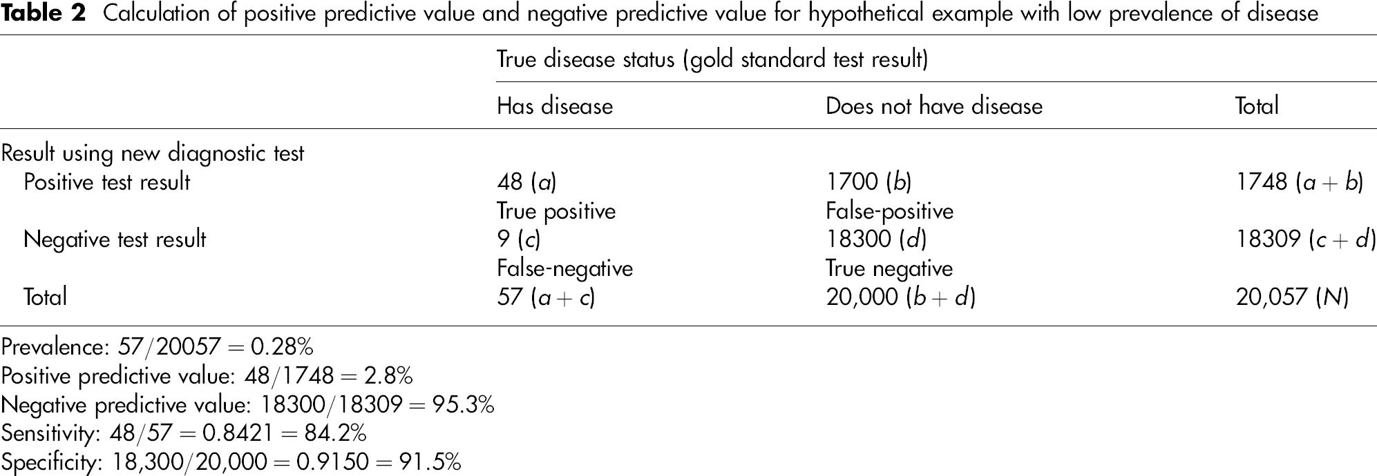
Prevalence: 57/20057 = 0.28%
Positive predictive value: 48/1748 = 2.8%
Negative predictive value: 18300/18309 = 95.3%
Sensitivity: 48/57 = 0.8421 = 84.2%
Specificity: 18,300/20,000 = 0.9150 = 91.5%
Hopefully, it is clear as to why this is the case. There are more individuals without the disease in the population, and therefore more false-positive results will occur. As a result, a smaller proportion of the positive tests will come from individuals who truly have the disease, and the PPV will be lower. It can be seen that the converse is true when considering the NPV. Thus, as the prevalence of a disease decreases, so the PPV decreases and the NPV increases.
Therefore, in this example, an individual with a positive test result still only has a 2.8% chance of having the disease. It is clear that if the prevalence of a disease is low in a population, the PPV will not be close to 100%, even if the test is excellent with a high sensitivity and specificity. This is particularly important for national screening programmes, where a large proportion of individuals with a positive test result will be false-positives. 2
The association between sensitivity, specificity, PPV and NPV
In the real-life clinical situation, it is unlikely that data such as those shown in Tables 1 and 2 are going to be available for every patient's situation. It is much more likely that the sensitivity and specificity of the test will be known as this information is transportable between patient populations. Furthermore, the prevalence (i.e. the probability that the individual being tested had the disease prior to the test being performed) is usually also known or can be estimated. With these three pieces of information, it is possible to obtain the PPV and NPV.
There are many ways of calculating the PPV and NPV from the prevalence, sensitivity and specificity. Exact (and relatively simple) formulae can be used, and these are given by Bland and Altman in their article on PPV and NPV 2 Furthermore, a nomogram that converts the prevalence (called here the pretest probability) into the PPV and NPV using the likelihood ratio (a combination of the sensitivity and specificity) is also widely available. 3
Conclusions
In the previous two Research design and statistics notes, we have considered important concepts when assessing the accuracy of a new diagnostic test. Up until now, we have considered the situation in which the test provides a binary test result (i.e. positive or negative). In the next Research design and statistics notes we shall consider the situation in which a diagnostic test provides an ordinal or numerical result (e.g. a laboratory marker). Here, we must choose a cut-off above (or below) which we will define an individual to have the disease or condition of interest. We shall consider how best to choose the cut-off, including the use of receiver operating curves.