The Impact of Institutional Grant Aid on College Choice

Abstract

In this study, I exploit exogenous differences in institutional policies regarding the treatment of home equity in grant aid allocation to estimate a causal impact of institutional grant aid on college choice. Because institutional grant aid is typically not awarded randomly, the college-estimated home equity value serves as an instrumental variable from which the causal relationship between institutional grant aid and college choice is identified. An additional $1,000 in institutional grant aid awarded by the typical sampled college increases the probability that the typical accepted student will choose that college by 1.66 percentage points. I also find that choice elasticity varies by student socioeconomic status, with the lowest income students nearly three times more sensitive to institutional grant aid than high-income students.

Keywords

instrumental variables college choice financial aid

Despite the ample literature addressing the admissions process by which American postsecondary institutions select students, there exists relatively little compelling research on how students choose which college to attend (Nurnberg, Schapiro, & Zimmerman, 2010). What limited literature on college choice exists suggests that distance between a student’s home and college as well as the highly associated factors of college quality, selectivity, and prestige are the most influential drivers in this decision (Avery, Glickman, Hoxby, & Metrick, 2005; Long, 2004).

Understanding the factors that influence college choice at selective postsecondary institutions is important because students’ college choices appear to be linked with other future outcomes. Specifically, economic returns to college may be related to college choice. Although there is not a clear consensus regarding the relationship between college selectivity and future earnings, the literature suggests that, at least for traditionally underrepresented students (e.g., low-income students), college selectivity is positively related to expected lifetime income (Dale & Krueger, 2002; Hoxby & Long, 1999). This relationship may be partially explained by the host of opportunities afforded to students attending the nation’s most selective postsecondary institutions. According to Eide, Brewer, and Ehrenberg (1998), a student’s choice to attend a more selective institution not only increases the probability of attending graduate school, it also increases the probability of attending a top graduate school. Along the same lines, Lentz and Laband (1989) show that college selectivity is positively related to medical school acceptance, even after controlling for relevant covariates like college grades, MCAT scores, parental education, and race. Persisting into the labor force, the signal associated with a student’s college choice even influences promotion within organizations, with graduates of more selective colleges ascending the corporate ladder more quickly than their peers from less selective institutions (Ishida, Spilerman, & Su, 1997). In addition, and possibly related to the direct economic impact of college choice, a student’s academic performance or persistence may suffer from making a “bad” college choice. For example, Okun, Levy, Karoly, and Ruehlman (2009) offer some evidence that unhappiness, a likely symptom of mismatch between student and institution, is negatively related to college GPA, and Aitken (1982) indicates that dissatisfied students are less likely to persist at their postsecondary institutions.

Yet, the institution is also vested in the student’s college choice. The influence that students exert on each other, termed peer effects, impacts the academic performance of these students. Causal evidence from roommate studies suggests that a student’s GPA tends to suffer if he or she is paired with an academically weaker roommate (Zimmerman, 2003). Moreover, these studies suggest that a student’s participation in social activities, like fraternities or sororities, is influenced by his or her roommate’s participation in these activities (Sacerdote, 2001). Consequently, a student’s college experience is shaped not only by inputs over which the institution has total control, like per student expenditures (Winston, 1999), but by the behavior and characteristics of the other students who enroll. A campus may not be enhanced by the presence of students who were induced to choose the college only because of enrollment incentives like generous grant aid and then are unhappy. Institutional motivations to provide such incentives may be prompted by concerns over college rank in national magazines like U.S. News and World Report. The rank order of colleges is determined by factors such as the test scores of the incoming class, and so colleges spend considerable time and effort attempting to convince their strongest candidates to accept offers of admission.

Background and Context

Institutional Grant Aid Distribution

By themselves, government initiatives to make college affordable through grant assistance programs (e.g., the Federal Pell Grant program) and subsidized loan programs (e.g., Perkins and Stafford loans) are incapable of offsetting the $50,000 sticker prices at the nation’s most selective private postsecondary institutions. However, to make college affordable to a broad segment of the American population, these institutions have adopted policies that result in—often very substantial—aid offers to supplement external financial assistance with institutional grant aid (Ehrenberg, 2000). Unlike government assistance, institutional aid packages awarded to a particular student can vary greatly across institutions with similarly stated commitments to affordability.¹

This variation exists for several reasons. First, some selective postsecondary institutions assist students by packaging loans, which must be repaid after graduation, while others have recently adopted policies to replace loans with additional awards of institutional grants (Linsenmeier, Rosen, & Rouse, 2006). Second, selective colleges differ in the formulae they use to calculate need. In most instances, to qualify for institutional grant aid, applicants must complete and submit the Free Application for Federal Student Aid (FAFSA) form. FAFSA information, which enumerates parental income and total assets, is then used to determine the student’s Estimated Financial Contribution (EFC). Among my sample of colleges, applicants are also required to supplement the FAFSA with the College Board–administered Financial Aid Profile. This form probes deeper into the applicant’s financial circumstances by collecting information on the parents’ home equity and noncustodial income (College Board, 2007). With a few notable exceptions like Harvard (Fitzsimmons, McGrath, & Donahue, 2009), selective postsecondary institutions do not disclose exactly how they determine institutional grant aid from these two sources. Finally, the professional judgment of financial aid officers may be used to adjust the awards that were determined by standard aid allocation formulae.

Home equity, measured as the value of the home(s) of the applicant and/or his or her parents minus the value of the home mortgage, is a major criterion that is prioritized differentially in the allocation of institutional grant aid across American colleges and universities. Only 12.5% of American 4-year postsecondary institutions require financial aid applicants to provide their family’s home value and mortgage debt (Tedeschi, 2009). Some selective, private institutions, like Harvard and Princeton, ignore wealth in the form of home equity when offering institutional grant aid to admitted students (Rimer & Finder, 2007). At the opposite end of the spectrum are selective, high-tuition institutions with relatively low endowments, like Sarah Lawrence College, which place no upper cap on the amount of home equity that can be considered in the determination of grant aid. Many other wealthy private colleges operate somewhere between these two extremes. Such schools expect parents to contribute a certain percentage of their home equity toward college costs, with the percentage and the upper caps differing across colleges (Roman, 2008; Tedeschi, 2009). For a given student, these policy differences create between-college variation in the amount of home equity considered by the college in the institutional grant allocation process. Consequently, a unique applicant may receive very different institutional grant aid awards across institutions with similar commitments to affordability.

Impact of Institutional Grant Aid on College Choice

Despite the scarcity of literature addressing the impact of institutional grant aid on postsecondary choice, there does exist a small body of literature on the impact of institutional grant aid on the probability of attending a particular institution (Linsenmeier et al., 2006; Monks, 2009; van der Klaauw, 2002). In each of these studies, the authors had access to admissions and financial aid data from one institution only. Therefore, it is unclear how much of the estimated increases in matriculation probability from an additional $1,000 in institutional grant aid are due to students choosing the focal college over another college versus the student choosing the focal college over not attending college at all.

Thus far, Avery and Hoxby (2003) offer the most compelling empirical study aimed at isolating the impact of institutional grant aid on choices between colleges. Their study influences the analytic approach I employ in this article. Using a sample of 3,240 high school seniors who planned to enter college in the fall of 2000, Avery and Hoxby incorporated a student’s “menu” of college choices into their statistical models. To do this, they applied McFadden’s choice model using the method of conditional logistic regression (CLR). This approach allowed them to eliminate variability in the outcome (choosing college j) attributable to differences in the characteristics of sampled individuals that are constant across schools (e.g., SAT scores, wealth). Avery and Hoxby also control for carefully selected characteristics of colleges, such as tuition and whether the college is public, by incorporating college-level covariates in their models. As a consequence of choosing this comprehensive analytic strategy, Avery and Hoxby estimate how much $1,000 of institutional grant aid from College X increases the odds of choosing College X conditional on the student’s other acceptances and institutional grant aid packages.

Avery and Hoxby’s (2003) claim that their estimates, which are reviewed in the discussion section of this article, are unbiased and can be interpreted causally is persuasive, and they certainly chose the best analytic approach given their data. In this study, I refine their analytic approach using more recently collected data to eliminate any potential sources of bias. I accomplish this in several ways. First, I rely on college administrative data rather than student-reported data. Second, I remove possible estimate contamination resulting from student negotiation of aid packages at their top choice colleges—a phenomenon that has the potential to bias estimates upwards. Finally, I remove downward bias stemming from preferential packaging in which colleges, with the intention of improving the yield of admitted students, award more grant aid to students perceived as less likely to attend if admitted.

In this study, I exploit exogenous variation in the way home equity is factored into institutional grant aid allocation to answer the following research questions.

Research Questions

Among a group of American citizens/permanent residents with multiple acceptances within a sample of 30 highly selective, private postsecondary institutions:

Research Question 1: By how much does an extra $1,000 in institutional grant aid given to students with demonstrated financial need increase the probability that the accepted student will choose the aid-granting college?

Research Question 2: Among students with demonstrated financial need, does the influence of institutional grant aid on student college choice differ by parental income? Specifically, is the impact greater for accepted students with lower parental incomes?

Research Design

Data Set

In this study, I use admissions and financial aid data from 30 highly selective private colleges and universities within a consortium that has served as the data source for periodic studies of admissions and financial aid processes (Hill & Winston, 2010; Hurwitz, 2011). Specifically, because this project focuses on college choice, I limit my data to American citizens or permanent residents who were accepted to at least two of the sampled colleges in the spring of 2009. This subsample includes 18,047 acceptances—the outcome variable—clustered within 6,306 students who were designated as “financially needy” by at least one of the sampled colleges. I do not have access to the complete set of colleges to which a student was admitted, which is a common limitation of administrative data, such as National Education Longitudinal Survey (NELS:88), used to examine college choice.² However, approximately 81% of the sampled students (84% of observations) matriculated at one of the sampled institutions in the fall of 2009. At least 1% deferred their matriculation until the fall of 2010.³ Students generally do not choose alternative postsecondary institutions outside of this sample, and as I show, the letters of admission and accompanying financial aid packages from these nonsampled institutions are unlikely estimate contaminants.

Sampled Colleges

Table 1 summarizes selected characteristics of the 30 sampled colleges and universities in comparison to a broader set of postsecondary institutions. Clearly, the sampled colleges’ characteristics do not mirror those of the average American 4-year, postsecondary institution, though their characteristics are fairly representative of the average institution in the top 100 of U.S. News and World Report rankings.

Table 1

Institution-Level Sample Statistics on Demographic and Financial Characteristics of Matriculants at the 30 Sampled Colleges Versus Matriculants at the Average School in the Top Ranking Tier of US News and World Report and the Average 4-year Postsecondary Institution

	Sample of colleges and universities	U.S. News and World Report top 50 liberal arts colleges and national universities	Public and private not-for-profit 4-year postsecondary institutions
Median SAT (M + CR)	1,422 (30)	1,317 (95)	1,101 (1,254)
Percentage receiving institutional grant aid	55.2 (30)	49.5 (101)	49.9 (1,915)
Mean institutional grant aid	$29,459 (30)	$16,508 (101)	$6,970 (1,861)
Mean out-of-state tuition and fees	$37,609 (30)	$31,727 (98)	$18,081 (2,031)
Percentage receiving federal grant aid	16.1 (30)	20.1 (101)	35.5 (1,915)
Percentage underrepresented minorities	16.7 (30)	15.6 (103)	24.4 (1,936)

Source. IPEDS; U.S. News and World Report Best Colleges 2010, 2011.

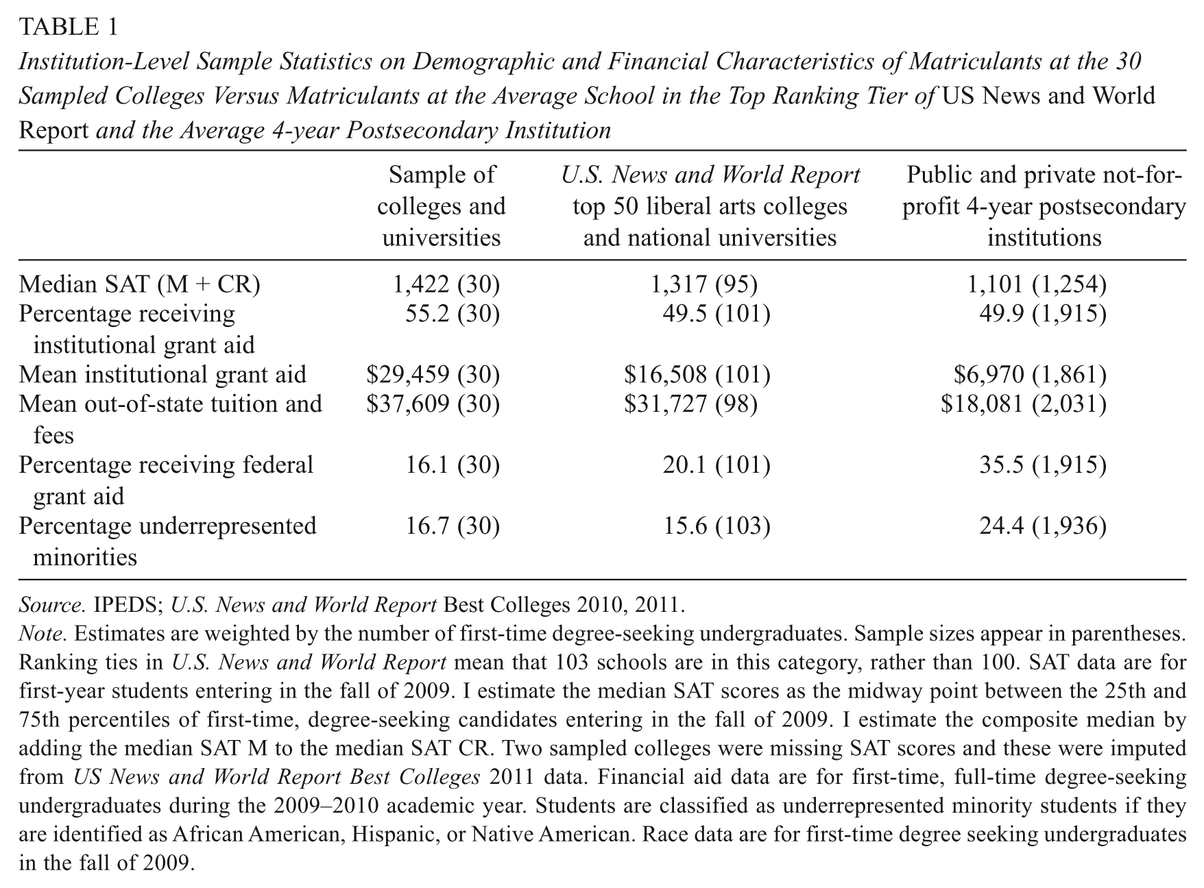
Note. Estimates are weighted by the number of first-time degree-seeking undergraduates. Sample sizes appear in parentheses. Ranking ties in U.S. News and World Report mean that 103 schools are in this category, rather than 100. SAT data are for first-year students entering in the fall of 2009. I estimate the median SAT scores as the midway point between the 25th and 75th percentiles of first-time, degree-seeking candidates entering in the fall of 2009. I estimate the composite median by adding the median SAT M to the median SAT CR. Two sampled colleges were missing SAT scores and these were imputed from US News and World Report Best Colleges 2011 data. Financial aid data are for first-time, full-time degree-seeking undergraduates during the 2009–2010 academic year. Students are classified as underrepresented minority students if they are identified as African American, Hispanic, or Native American. Race data are for first-time degree seeking undergraduates in the fall of 2009.

A possible limitation of focusing only on highly selective postsecondary institutions is that the students choosing among these institutions may respond differently to grant aid than their peers choosing among less selective postsecondary institutions. The existence of such a phenomenon would suggest that the results of this study are not generalizable to the typical college-bound student. I explore this possibility in the sensitivity analyses and find some evidence to discount this threat, yet the choice to focus on this particular set of elite colleges must be justified.

Aggressive application behavior among highly talented students results in thousands of students with multiple admissions offers at a similar set of highly selective colleges. It is just this similarity in college choice sets that drives the methodology from which I draw my conclusions. Because less competitive students are more likely to apply to fewer and more regional postsecondary institutions (Bound, Hershbein, & Long, 2009; Hoxby, 2009), finding a set of students with enough overlap in college options and then convincing these sets of overlapping colleges, which traditionally do not share data with each other, to surrender their admissions and financial aid records is perhaps an insurmountable obstacle. Therefore, it is likely that any such study addressing college choice behavior would, out of necessity, focus on highly competitive colleges.

Measures

In my data set, each acceptance contributes one row of data, and students are represented in multiple rows.

Outcome:

CHOICE_ij. A dichotomous variable that is coded 1 if applicant i chooses to matriculate at institution j (1=matriculates; 0, otherwise).

Instrument:

EST_HOMEEQUITY _ij. The total amount of home equity considered by college j in its grant aid allocation process.

Endogenous predictors:

INSTGRANT _ij. A continuous variable describing the institutional grant aid awarded to applicant i at institution j (in $1,000s).

Fixed effects:

STUDENT_i. A vector of dummy variables distinguishing each applicant.

COLLEGE_j. A vector of 30 dichotomous variables that distinguishes the 30 sampled colleges. The jth component of the COLLEGE vector is coded 1 if the acceptance was from the jth college (0, otherwise).

Control predictors:

LEGACY_ij. A dichotomous variable that is coded 1 if the student has any familial ties to the outcome college (0, otherwise).

GEODIST_ij. A continuous variable that equals the distance between student i’s home and college j.

Interaction predictor:

INCAT_i. A vector of six dichotomous variables that represents the total income (INCOME), as reported by the college, of a student’s parents in 2008 (or estimated for 2009). Each dichotomy, except INCAT6, spans $50,000. For example, INCAT1 is set to 1 if applicant i has a parental income between $0 and $50,000, otherwise INCAT1 = 0 for student i. INCAT6 equals 1 if parental income is greater than $250,000.

TIER1 (most selective), TIER2, TIER3, TIER4 (least selective). Four dichotomous variables (e.g., TIER1) with each coded to 1 if COLLEGE_j is in the specified selectivity tier (e.g., TIER1) (0, otherwise).⁴

Data Analysis

Methodology

In this study, I use two methodological approaches simultaneously to examine my research questions. As previously noted, institutional grant aid is not awarded randomly; therefore, any straightforward analysis linking institutional grant aid amounts to college choices, such as regressing institutional grant aid at one institution on the probability of choosing that institution, would be biased. At the sampled colleges, institutional grant amounts vary due to policy differences, which I argue are exogenous, in the way these colleges treat home equity in the student’s need calculation. Specifically, the home equity considered by a particular college impacts college choice only through the variation in institutional grant aid created by this metric and therefore serves as an instrumental variable through which I may estimate an unbiased effect of institutional grant aid on college choice.

The second methodological approach, which I implement within the instrumental variable framework discussed previously, involves the incorporation of fixed effects for students and outcome colleges into all statistical models. While differences in college-estimated home equity are a large source of between-college variation in institutional grant aid for a given student, other sources of between-college variation in institutional grant aid exist. However, unlike college-estimated home equity, which effectively results from the interaction of actual home equity and college financial aid policy, these variations arise because of differences in student-level characteristics that are constant across colleges. Failing to control for the fixed effects of students would create the illusion that aid packages are distributed solely based on the home equity considered, when other predictors of aid like family income and net worth are clearly important in aid allocation across all sampled colleges. Although 19% of sampled students do not ultimately choose a sampled college, these students are preserved in the analyses because they inform the relationship between home equity considered and institutional grant aid.

The importance of including fixed effects for colleges is illustrated in Figure 1, which shows the relative odds of choosing a sampled college over other sampled colleges, by selected college-level characteristics. Even after accounting for institutional grant aid offered, there is enormous variation in the appeal of the sampled colleges. Given the choice between college S12 and college S25, the typical student is 150 times more likely to choose school S12, with an odds ratio of 1,500, over school S25, with an odds ratio of 10. Odds ratios, rather than probabilities, are presented in Figure 1 to convey the magnitude of differences in the sampled colleges’ desirability. Not only are more selective/wealthy colleges more appealing, they tend to have more lenient policies with respect to home equity consideration. Figure 2 shows the across-college variation in home equity considered for the typical sampled admit, with an actual home equity of about $200,000, and demonstrates quite clearly that wealthy/more selective colleges tend to consider less home equity in the aid allocation process than their less selective peers. However, sampled colleges, for the most part, only compete for admitted students with their nearest neighbors on these selectivity/wealth dimensions. Among nearest neighbors, home equity consideration policies are exogenous to student choice, as I show in the sensitivity analyses.

Figure 1.

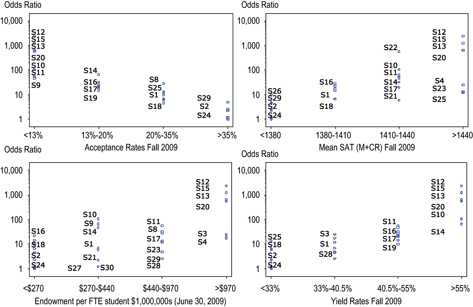
Relative college choice odds.

Figure 2.

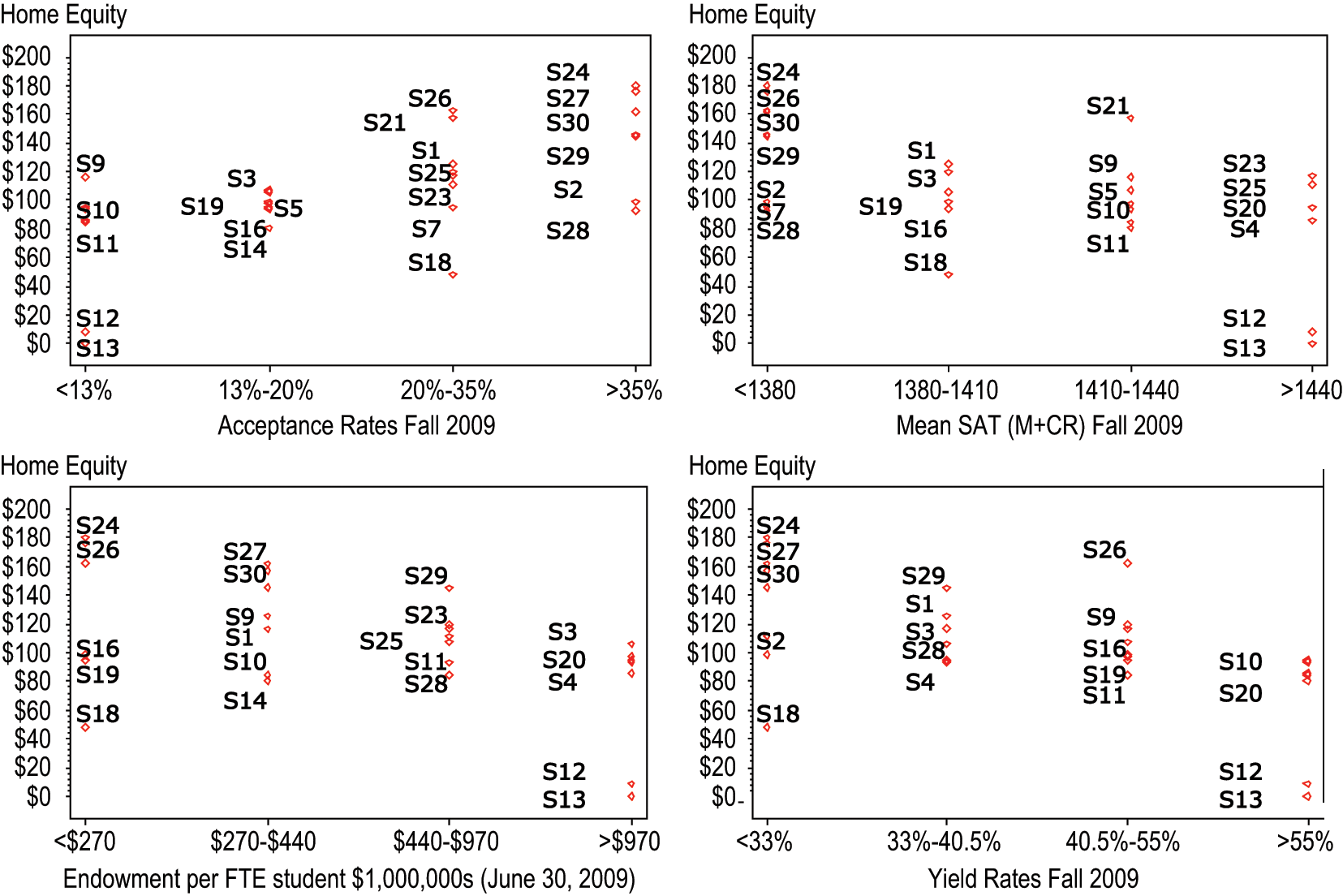
College-estimated home equity for typical sampled admit ($1,000s)

Conditional logistic regression, the analytic approach traditionally used in the study of college choice (Avery & Hoxby, 2003; Long, 2004; Manski & Wise, 1983), also achieves the goal of eliminating variability in outcome attributable to student-level characteristics that do not vary across the student’s college opportunity set (e.g., race, SAT scores, GPA). Rather than estimating parameters for a vector of student fixed effects, CLR allows for an intercept term that differs across strata (Allison, 2005). Ideally, I would conduct my instrumental-variable estimation within a CLR framework in order to account for the fact that my ultimate outcome, college choice, is dichotomous. This proposed technique, while effective in theory, presents one major drawback—there is no known method of implementing it in the context of instrumental variables estimation, which I require in order to obtain unbiased estimates of choice elasticity (Geyer & Thompson, 1992; Murnane & Willett, 2011). As an alternative, I estimate the impact of institutional grant aid on college choice by specifying a linear probability (LP) model at the second stage, with fixed effects for both schools and students, and substituting the actual INSTGRANT values for the predicted INSTGRANT values to correct the second-stage standard errors (Murnane & Willett, 2011). Concerns associated with using an LP model, rather than a logistic model (Horrace & Oaxaca, 2006), are offset by evidence that in large samples, parameter estimates obtained from LP estimation tend to be asymptotically unbiased (Angrist & Pischke, 2009; Betts & Fairlie, 2001).

Research Questions

To answer this research question, I use two-stage least squares (2SLS) estimation to fit the following statistical models for applicant i at college j.

1^{s t} s t a g e : I N S T G R A N T_{i j} = ω ’ S T U D E N T_{i} + γ ’ C O L L E G E_{j} + δ_{1} E S T_H O M E E Q U I T Y_{i j} + ε_{i j}

2^{n d} s t a g e : C H O I C E_{i j} = τ ’ S T U D E N T_{i} + θ ’ C O L L E G E_{j} + β_{1} {\overset{⌢}{I N S T G R A N T}}_{i j} + μ_{i j}

In the first-stage model, controlling for the fixed effects of student and college, I regress institutional grant aid on the college estimated home equity used for institutional grant aid allocation. In the second-stage model, I regress college choice on the predicted institutional grant aid obtained from the first-stage model while continuing to control for the fixed effects of student and college. Regression parameter β₁ represents the increase in probability that accepted student i chooses to matriculate at college j, over his or her other college options within the sampled colleges, due to an increase of $1,000 in institutional grant aid at college j.

To answer this question, I again use an instrumental variable estimation strategy. The final equation (Equation 9) contains six endogenous interaction terms between INSTGRANT and INCAT. Therefore, I instrument for each of these six endogenous interaction terms with six interaction terms between EST_HOMEEQUITY and INCAT (Equations 3 through 8).

I N S T G R A N T_{i j} * I N C A T 1_{i} = ω_{1} ’ S T U D E N T_{i} + γ_{1} ’ C O L L E G E_{j} + \sum_{k = 1}^{6} (δ_{1 k} E S T_H O M E E Q U I T Y_{i j} * I N C A T k_{i}) + ε_{1 i j}

I N S T G R A N T_{i j} * I N C A T 2_{i} = ω_{2} ’ S T U D E N T_{i} + γ_{2} ’ C O L L E G E_{j} + \sum_{k = 1}^{6} (δ_{2 k} E S T_H O M E E Q U I T Y_{i j} * I N C A T k_{i}) + ε_{2 i j}

I N S T G R A N T_{i j} * I N C A T 3_{i} = ω_{3} ’ S T U D E N T_{i} + γ_{3} ’ C O L L E G E_{j} + \sum_{k = 1}^{6} (δ_{3 k} E S T_H O M E E Q U I T Y_{i j} * I N C A T k_{i}) + ε_{3 i j}

I N S T G R A N T_{i j} * I N C A T 4_{i} = ω_{4} ’ S T U D E N T_{i} + γ_{4} ’ C O L L E G E_{j} + \sum_{k = 1}^{6} (δ_{4 k} E S T_H O M E E Q U I T Y_{i j} * I N C A T k_{i}) + ε_{4 i j}

I N S T G R A N T_{i j} * I N C A T 5_{i} = ω_{5} ’ S T U D E N T_{i} + γ_{5} ’ C O L L E G E_{j} + \sum_{k = 1}^{6} (δ_{5 k} E S T_H O M E E Q U I T Y_{i j} * I N C A T k_{i}) + ε_{5 i j}

I N S T G R A N T_{i j} * I N C A T 6_{i} = ω_{6} ’ S T U D E N T_{i} + γ_{6} ’ C O L L E G E_{j} + \sum_{k = 1}^{6} (δ_{6 k} E S T_H O M E E Q U I T Y_{i j} * I N C A T k_{i}) + ε_{6 i j}

C H O I C E_{i j} = τ ’ S T U D E N T_{i} + θ ’ C O L L E G E_{j} + β_{1} I N S T G R A N T_{i j} * I N C A T 1_{i} + β_{2} I N S T G R A N T_{i j} * I N C A T 2_{i} + β_{3} I N S T G R A N T_{i j} * I N C A T 3_{i} + β_{4} I N S T G R A N T_{i j} * I N C A T 4_{i} + β_{5} I N S T G R A N T_{i j} * I N C A T 5_{i} + β_{6} I N S T G R A N T_{i j} * I N C A T 6_{i} + σ_{i j}

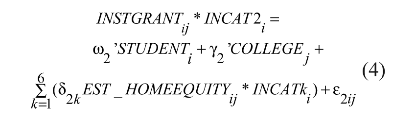
In Equation 9, β₁ represents the choice elasticity for individuals with parental incomes less than $50,000 (INCAT1 = 1); β₂ represents the choice elasticity for individuals with parental incomes between $50,000 and $100,000 (INCAT2 = 1), and so forth.

Findings

The Overall Impact of Institutional Grant Aid on College Choice

For almost all sampled colleges, EST_HOMEEQUITY is a key variable in the aid allocation process, even in the wake of the housing market crash affecting many students. Therefore, it is an extremely powerful instrument and a strong predictor of institutional grant aid (F statistic = 174).

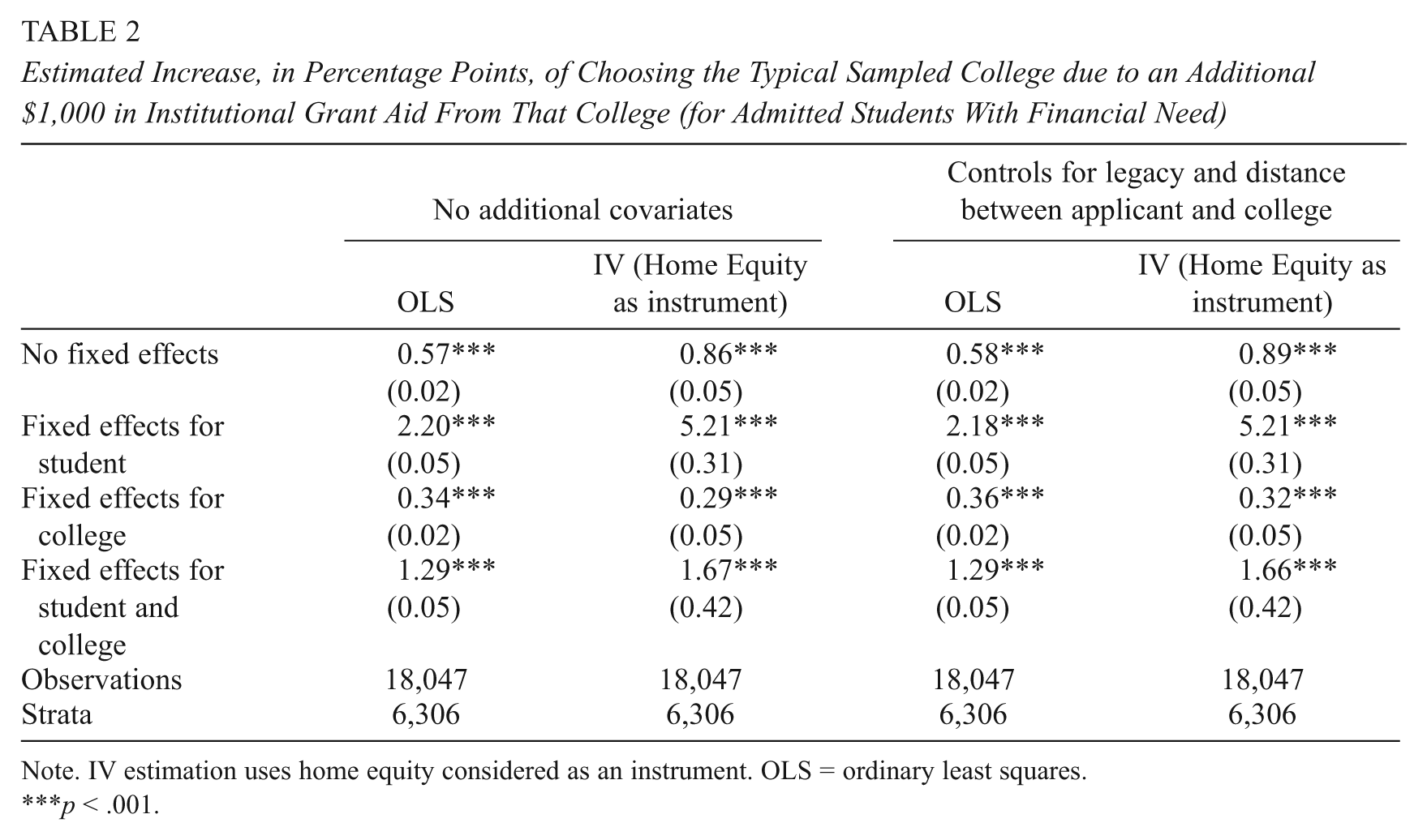
In Table 2, I present the increase, in percentage points, of choosing the typical sampled college due to an additional $1,000 in institutional grant aid from that college. I conclude that at the typical sampled college, an additional $1,000 increases the probability that a student will choose that college by 1.66 percentage points. This unbiased estimate represents parameter β₁ in Equation 2. As illustrated in Figure 1, schools with higher SAT scores tend to be more preferable, even after accounting for net price. In fact, refitting Equation 2 only by replacing the fixed effects of college with covariates for net price and institutional mean SAT scores reveals that offering an additional $1,000 in institutional grant aid, in terms of student preferences, is roughly equivalent to an institution increasing its mean SAT (M + CR) score by 5 points.

Table 2

Estimated Increase, in Percentage Points, of Choosing the Typical Sampled College due to an Additional $1,000 in Institutional Grant Aid From That College (for Admitted Students With Financial Need)

	No additional covariates		Controls for legacy and distance between applicant and college
	OLS	IV (Home Equity as instrument)	OLS	IV (Home Equity as instrument)
No fixed effects	0.57***	0.86***	0.58***	0.89***
	(0.02)	(0.05)	(0.02)	(0.05)
Fixed effects for student	2.20***	5.21***	2.18***	5.21***
	(0.05)	(0.31)	(0.05)	(0.31)
Fixed effects for college	0.34***	0.29***	0.36***	0.32***
	(0.02)	(0.05)	(0.02)	(0.05)
Fixed effects for student and college	1.29***	1.67***	1.29***	1.66***
	(0.05)	(0.42)	(0.05)	(0.42)
Observations	18,047	18,047	18,047	18,047
Strata	6,306	6,306	6,306	6,306

Note. IV estimation uses home equity considered as an instrument. OLS = ordinary least squares.

***

p < .001.

Alongside this unbiased estimate, I present the percentage point increase estimate that would have been obtained if I had substituted into Equation 2 the actual institutional grant aid amount for student i at college j rather than the predicted institutional grant aid from Equation 1.⁵ If I were unable to find a suitable instrumental variable, the best analytic strategy for obtaining choice elasticity would have been to simply control for all student-level characteristics that are constant across colleges (fixed effects for student) and all college-level characteristics that are constant across students (fixed effects for colleges). This value (1.29 percentage points per $1,000 in institutional grant aid) represents a biased ordinary least squares (OLS) estimate of choice elasticity.

Like institutional grant aid, legacy status and distance between the student and the college are not constant across the menu of college options faced by the student and consequently are neither controlled for through the fixed effects of students nor the fixed effects of colleges. Shown in prior research to be influential in the colleges’ admissions processes (Hurwitz, 2011), legacy status also proves to be a significant predictor of a student’s choice process (F = 24.80, p < .0001) when added to Equation 1 and Equation 2. Similarly, increases in distance between student and college, which have been shown to impact adversely the decision to apply to selective colleges (Griffith & Rothstein, 2009), also negatively impact the probability of choosing a particular college (F = 4.88, p = .027) conditional on all applicant and college invariant characteristics as well as institutional grant aid.

If colleges were to award more grant aid to legacies (for example) because of their legacy status and these students were also more inclined to choose the school at which they enjoy legacy status (conditional on grant aid), such preferential packaging conceivably could distort the relationship between home equity considered and institutional grant aid, weakening the instrument used to obtain unbiased instrumental variable (IV) estimates. Fortunately, these concerns are unfounded. Comparing the second and fourth columns as well as the first and third columns in Table 2 reveals that including the LEGACY and GEODIST covariates in Equations 1 and 2 bears no impact on the OLS or IV estimates. This reassuring finding strongly supports the assumption that any other student characteristics that differ across the student’s choice set (e.g., quality of college-specific essays) would also not alter the choice elasticity estimates in Table 2.

Differences in the Impact of Institutional Grant Aid Across the Socioeconomic Spectrum

Measuring a student’s socioeconomic status (SES) is particularly tricky, and while parental income may not provide a complete picture of a student’s financial circumstances, historically, it is a commonly used metric in determining socioeconomic status (Entwisle & Astone, 1994). Yet even a term as basic and ubiquitous as income is challenging to define, and the sampled colleges illustrate this through the across-college differences in income components that are used to determine financial need. In addition to custodial parents’ wages, such components might include noncustodial parental wages, capital gains, business income, trust income, and rental income, in addition to untaxed income like child support, welfare benefits, veteran’s benefits, pensions, and so forth. In order to address how the impact of institutional grant aid on choice elasticity varies across the student socioeconomic spectrum, I need to estimate the student’s true parental income—a variable that is constant across the schools to which a student was accepted. The challenge in such an estimation process is that for nearly 90% of the sampled students, the considered parental income varies across colleges. Ideally, all sampled colleges would report each component of the student’s true parental income, even if the specific component were not used in the aid allocation process. Unfortunately, colleges do not have a common standard for such data collection and record-keeping; therefore, I impute a student’s parental income as the maximum parental income considered from the set of colleges to which the student was accepted. I contend that the maximum within-student income most closely reflects a student’s true parental income and is most representative of his or her socioeconomic status.

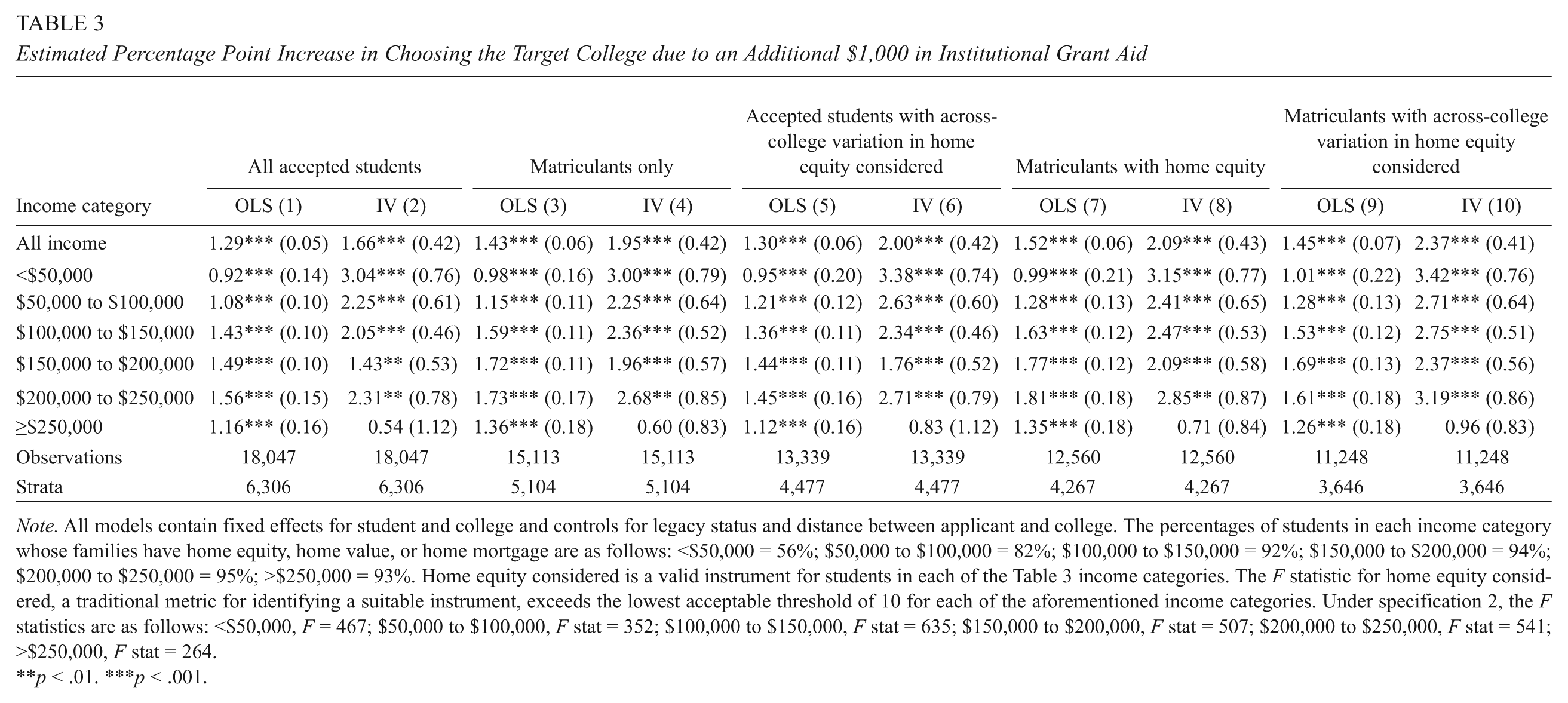
In these analyses, I have created six student-level parental income categories, each spanning $50,000, with the exception of the highest income category, which includes all students with a maximum parental income greater than $250,000. The width of the resulting income categories align quite nicely with the 2009 median household income of $49,777 (DeNavas-Walt, Proctor, & Smith, 2010). The choice to create a categorical rather than a continuous income variable was motivated by the fact that the relationship between choice elasticity and income is not monotonic. In Table 3, I present the choice elasticity estimates by parental income calculated through the IV approach represented by Equations 3 through 9 and through an OLS approach.

Table 3

Estimated Percentage Point Increase in Choosing the Target College due to an Additional $1,000 in Institutional Grant Aid

	All accepted students		Matriculants only		Accepted students with across-college variation in home equity considered		Matriculants with home equity		Matriculants with across-college variation in home equity considered
Income category	OLS (1)	IV (2)	OLS (3)	IV (4)	OLS (5)	IV (6)	OLS (7)	IV (8)	OLS (9)	IV (10)
All income	1.29*** (0.05)	1.66*** (0.42)	1.43*** (0.06)	1.95*** (0.42)	1.30*** (0.06)	2.00*** (0.42)	1.52*** (0.06)	2.09*** (0.43)	1.45*** (0.07)	2.37*** (0.41)
<$50,000	0.92*** (0.14)	3.04*** (0.76)	0.98*** (0.16)	3.00*** (0.79)	0.95*** (0.20)	3.38*** (0.74)	0.99*** (0.21)	3.15*** (0.77)	1.01*** (0.22)	3.42*** (0.76)
$50,000 to $100,000	1.08*** (0.10)	2.25*** (0.61)	1.15*** (0.11)	2.25*** (0.64)	1.21*** (0.12)	2.63*** (0.60)	1.28*** (0.13)	2.41*** (0.65)	1.28*** (0.13)	2.71*** (0.64)
$100,000 to $150,000	1.43*** (0.10)	2.05*** (0.46)	1.59*** (0.11)	2.36*** (0.52)	1.36*** (0.11)	2.34*** (0.46)	1.63*** (0.12)	2.47*** (0.53)	1.53*** (0.12)	2.75*** (0.51)
$150,000 to $200,000	1.49*** (0.10)	1.43** (0.53)	1.72*** (0.11)	1.96*** (0.57)	1.44*** (0.11)	1.76*** (0.52)	1.77*** (0.12)	2.09*** (0.58)	1.69*** (0.13)	2.37*** (0.56)
$200,000 to $250,000	1.56*** (0.15)	2.31** (0.78)	1.73*** (0.17)	2.68** (0.85)	1.45*** (0.16)	2.71*** (0.79)	1.81*** (0.18)	2.85** (0.87)	1.61*** (0.18)	3.19*** (0.86)
≥$250,000	1.16*** (0.16)	0.54 (1.12)	1.36*** (0.18)	0.60 (0.83)	1.12*** (0.16)	0.83 (1.12)	1.35*** (0.18)	0.71 (0.84)	1.26*** (0.18)	0.96 (0.83)
Observations	18,047	18,047	15,113	15,113	13,339	13,339	12,560	12,560	11,248	11,248
Strata	6,306	6,306	5,104	5,104	4,477	4,477	4,267	4,267	3,646	3,646

Note. All models contain fixed effects for student and college and controls for legacy status and distance between applicant and college. The percentages of students in each income category whose families have home equity, home value, or home mortgage are as follows: <$50,000 = 56%; $50,000 to $100,000 = 82%; $100,000 to $150,000 = 92%; $150,000 to $200,000 = 94%; $200,000 to $250,000 = 95%; >$250,000 = 93%. Home equity considered is a valid instrument for students in each of the Table 3 income categories. The F statistic for home equity considered, a traditional metric for identifying a suitable instrument, exceeds the lowest acceptable threshold of 10 for each of the aforementioned income categories. Under specification 2, the F statistics are as follows: <$50,000, F = 467; $50,000 to $100,000, F stat = 352; $100,000 to $150,000, F stat = 635; $150,000 to $200,000, F stat = 507; $200,000 to $250,000, F stat = 541; >$250,000, F stat = 264.

p < .01. ***p < .001.

Not all sampled individuals have variation in the outcome measure, college choice, and the instrument, home equity considered. The sample restrictions in Table 3 are included to reassure readers that results are robust to the exclusion of accepted students not meeting the two criteria above. Although the IV estimates for the whole sample (specification 2) represent a local average treatment effect on matriculants with variation in home equity considered, preserving both matriculants and nonmatriculants without variation in the instrument serves to define the relative generosity of the sampled colleges. These students indirectly impact choice elasticity estimates by contributing to the college fixed effects parameter estimation in the first-stage equations. Similarly, matriculating students with no variation in home equity considered serve to define the relative desirability of the sampled colleges, contributing to the estimation of college fixed effects parameters at the second stage. Although selective omission of these subgroups does not appear to dramatically alter this article’s results, discarding informative data not meeting the two aforementioned criteria may not be a sensible decision.

Table 3 conveys that below the $200,000 income threshold, the IV choice elasticity estimates tend to decrease as parental income increases. Among students with parental incomes less than $50,000 per year, an additional $1,000 in institutional grant aid awarded by the typical sampled college increases the probability that the student will choose that college by 3.04 percentage points. Among the wealthiest sampled students—those with parental incomes greater than or equal to $250,000—the choice elasticity is only .54, an estimate that is not significantly different from zero (specification 2).

Across the six income categories in Table 3, I am unable to reject the hypothesis that the unbiased choice elasticity estimates are jointly equal in specification 2 (F = 1.20, p = .31). This may be attributable to the vacillation in choice elasticity above the $200,000 parental income threshold. However, among the 84% of sampled students (see Figure 3 for sampled student income distribution) who constitute the four lowest income categories, the choice elasticity appears to be negative and linear.

Figure 3.

Distribution of parental income

Because of this apparent monotonicity, I refit IV models⁶ treating INCOME as a continuous variable to obtain an unbiased estimate of choice elasticity within this income range. When the sample is restricted to only students with family incomes less than $200,000 per year and INCOME is treated as a continuous linear variable, I find that a $50,000 increase in income is associated with a .6 percentage point decrease in choice elasticity (t = −2.37, p = .018). Figure 4 shows the estimated choice elasticity against family income when income is treated as a continuous variable. All relationships presented in Figure 4, including those with higher-order terms for income to allow for nonlinearity, depict a strong negative relationship between choice elasticity and family income below the $200,000 threshold.

Figure 4.

Choice elasticity by parental income

The second major take-home message from Table 3 is that the OLS and the IV estimates depict different stories about the relationship between income and choice elasticity. Specification 1 in Table 3 contains the OLS estimates that I would have obtained had I not found a suitable instrument. In contrast to the IV estimates, I can reject the hypothesis that the biased OLS estimates are jointly equal across the six income categories in specification 1 of Table 3 (F = 4.14, p = .0009). According to this OLS analysis, which is analogous to Avery and Hoxby’s (2003) conditional logit analysis of grant aid’s impact on college choice, middle-income students are most sensitive to institutional grant aid. Avery and Hoxby also found some evidence of this in their study.

The final point established in Table 3 is that for the lowest income students, the OLS estimates are biased downwardly. Tempting as it may be to infer this bias by comparing the IV estimate in specification 2 to the OLS estimate in specification 1, it is important to keep in mind that this IV estimate represents a local average treatment effect for matriculants with variation in home equity considered. Instead, a more appropriate comparison to infer OLS bias might be made from the subset of matriculants with variation in home equity considered (specifications 9 and 10). Among students with parental incomes less than $50,000 per year, no overlap exists between the 95% confidence interval associated with the IV estimate in specification 10 and the OLS estimate in specification 9, confirming that OLS estimates are biased downwardly for the lowest income students. Incidentally, this absence of overlap between the OLS and IV estimate confidence intervals occurs across all subgroups of accepted students with annual parental incomes less than $50,000.

Discussion

Comparing the OLS and IV Estimates of Choice Elasticity

The similarity between the OLS-estimated (with fixed effects for student and college) choice elasticity and the corresponding IV-estimated choice elasticity across the entire sample generally supports the conclusion of Avery and Hoxby (2003) that controlling for student-level characteristics that are constant across all colleges in addition to selected college-level attributes (or in my case, all college-level attributes that are constant across students) is sufficient to achieve unbiased estimates of choice elasticity.

Among the individuals in the sample with family incomes less than $50,000 per year, the IV estimates of choice elasticity are markedly higher than the corresponding OLS estimates.

Identifying conclusively the mechanism driving these differences between the OLS estimates and the IV estimates is beyond the scope of this project and simply not possible given the data. Yet speculating about possible drivers should serve to motivate future research. One plausible source of endogeneity, which might force a downward bias on the OLS estimates, is the awarding of more aid to students perceived as less interested in matriculating. Gauging student interest has become so commonplace among colleges that they are asked to rate its importance in admissions in the annually published Common Data Set Initiative. Theoretical models addressing the relationship between binding early decision processes and financial aid hint that the most interested applicants, as evidenced by applying early decision rather than regular decision, may receive inferior aid packages (Kim, 2010). Even though no definitive evidence exists that any of the sampled colleges consider student interest in aid allocation, seasoned college admissions consultants reiterate that schools engage in preferential aid packaging, even if they claim that the aid allocation process is strictly driven by financial well-being (Wong, 2005).

An upward bias in the OLS estimates would arise from a student lobbying and ultimately receiving more generous aid packages at the most desirable colleges in his or her choice set. This upward bias stems from the fact that some students would have matriculated at their final-choice colleges even in the absence of upwardly revised grant aid packages. Because the grant aid packages in my study are the final grant aid packages, I am unable to ascertain the magnitude or frequency of such revisions. Avery and Hoxby (2003) note that this source of endogeneity occurred in about 9% of students in their sample, and this percentage has almost certainly increased over the past decade as more schools are willing to indulge such student requests (Kelley, 2010).

Negotiating student aid packages requires a certain amount of savvy on the part of students and families. Cultural capital with respect to the college application and college choice process differs markedly between the low SES students and their higher SES counterparts (McDonough, 1997; Perna, 2006). Parents of higher SES students may be more aware of their ability to leverage financial aid offers, and even if higher SES parents lack exposure to the selective college admissions and aid processes, their children are more likely to attend high schools with well-informed and seasoned staff who can supplement parental knowledge. Therefore, this type of post hoc negotiation is likely to occur most frequently among the wealthier financial aid recipients.

It is likely, though not provable, that these two sources of bias are operating simultaneously. Across the entire sample, the OLS estimate tends to be biased downwardly, suggesting that preferential packaging trumps negotiation as a source of bias. However, the shrinking gap between the OLS and IV estimates with increasing income (Table 3) is consistent with the theory of heightened negotiation frequency among higher income students relative to their lower income peers.

Comparing Elasticity Estimates Across Studies

With the exception of Avery and Hoxby (2003), all studies investigating student responsiveness to institutional grant aid have focused on enrollment elasticity—the increased probability that a student will enroll at the sampled college due to an additional $1,000 in institutional grant aid—rather than choice elasticity. All subsequently discussed elasticities are converted to 2009 dollars, explaining why these elasticities differ from those presented in the original papers.

The distinction between these two elasticity classifications is subtle, and they only differ in that estimation of enrollment elasticity does not parse out the component of student responsiveness due to the student choosing the sampled college over his or her other options versus choosing the sampled college over not attending college at all. In several studies of enrollment elasticity (e.g., Monks, 2009; van der Klaauw, 2002), the chosen identification strategies allow for the assumption that the grant aid packages at competitor institutions are identical between the study’s treatment (received additional grant aid) and control groups. Under such circumstances, if students were only choosing between postsecondary institutions, causal estimates of enrollment elasticity and causal estimates of choice elasticity should be identical.

At the nation’s more selective institutions, it is unlikely that many (or any) students are seriously balancing the two options of attending that selective postsecondary institution with not attending college at all. Therefore, the assumption of interchangeability between choice elasticity and enrollment elasticity at these types of institutions is justifiable. Such a statement warrants proof, and van der Klaauw’s (2002) study supplies compelling evidence to support this contention. Using a regression discontinuity framework, van der Klaauw finds that among financial aid filers, an additional 10% increase in institutional grant aid leads to an 8.6% increase in matriculation probability. In the context of my study, this estimate would translate into about a 1 percentage point increase in matriculating at one of the sampled colleges due to an additional $1,000 in institutional grant aid. While van der Klaauw’s estimate is similar to this study’s choice elasticity estimate, it is expectedly smaller because of his incorporation of some financial aid filers who may not have been eligible for need-based aid—a group of wealthier students who were excluded from my sample. Among nonfilers, van der Klaauw finds virtually no effect of institutional grant aid on enrollment probability, which is consistent with my finding that wealthy students are less sensitive to institutional grant aid. Monks (2009) confirms this weak sensitivity to aid among wealthier students by exploiting a natural experiment in which students ineligible for need-based aid were randomly awarded merit scholarships, through which he finds an enrollment elasticity of about .4.

Despite the fact that at the institution level enrollment elasticity and choice elasticity should not be treated as one and the same—except perhaps at the nation’s most selective postsecondary institutions—some evidence exists that student responsiveness to institutional grant aid when choosing between colleges is similar in magnitude to student responsiveness to grant aid when deciding whether to enroll in college at all. Dynarski (2003) exploits the termination of the Social Security Administration’s college payment program in 1982 for children of deceased, disabled, or retired social security beneficiaries to conclude that $1,000 ($2009) in grant aid leads to an increase in probability that the student will enroll in postsecondary education by 2.9 percentage points. Though Dynarski’s elasticity is larger than this study’s overall choice elasticity of 1.66, the typical student impacted by this abrupt policy shift had a family income of about $40,000 ($2009). I find that students with a comparable income to those impacted by this Social Security policy change have a choice elasticity of about 3—an estimate strikingly similar to that found by Dynarski. In yet another study, Dynarski (2000) explores the impact of Georgia’s Hope scholarship on college attendance and concludes that an additional $1,000 ($2009) in institutional grant aid increased the college attendance rate among Georgia’s students by 2.8 to 3.2 percentage points. Again, these enrollment elasticity estimates are higher than the average choice elasticity estimate in this study; however, Dynarski’s (2000) estimates are in the range of those illustrated in Table 3.

In the only other recent study of choice elasticity, Avery and Hoxby (2003) find a choice elasticity of approximately 1.5 ($2009) among students entering college in the fall of 2000. Despite using an identification strategy that is not causal under the most stringent criteria, Avery and Hoxby’s chosen analytic strategy likely generates an unbiased estimate of choice elasticity across their entire sample of students—though perhaps not when choice elasticity estimates are disaggregated by income. Furthermore, their overall choice elasticity is nearly identical to that revealed in this study.

As more studies investigating the impact of grant aid on college-specific enrollment, college attendance, and college choice are added to the corpus of academic literature, evidence of similarity in elasticity estimates is accumulating. Despite the small variations in elasticity estimates across samples, there appears to be no clear trends in the trajectories of these estimates over time. The differing samples and analytic strategies utilized by these studies forces me to stop short of declaring that student responsiveness to aid has been constant over the past 30 years or so; however, the collective evidence is certainly consistent with such a hypothesis.

Implications for the Student

Figure 5 shows that grant aid from all sources nearly covers the entire cost of attendance for students with the lowest family incomes. Even though these students are receiving the largest grant aid packages, they remain the most sensitive to additional institutional grant aid during the college choice process (Table 3). This may be related to the fact that lower income students perceive that they still have financial need beyond the package offered in spite of the generous aid provided by the sampled schools.

Figure 5.

Interquartile range of total grant aid as a percentage of student budget

The commitment to need-based aid is strongest at the nation’s most selective 4-year institutions, where roughly 90% of all institutional grant aid goes to meet need. As school selectivity decreases, so does the fraction of institutional grant aid used to meet student need. At nonselective, private, nonprofit 4-year colleges, 30% of institutional grant aid is strictly merit based, and at the nonselective 4-year public institutions, more than half of institutional grant aid is merit based (Baum & Payea, 2011). Although the majority of institutional grant aid is used to meet need, many colleges use merit aid as a tool intended for yield enhancement. This article offers no evidence that wealthy students respond to grant aid, and somewhat ironically, the institutions offering merit aid could probably achieve even higher yields on admitted students if this aid were redirected to the neediest students.

Perhaps most importantly, the findings of this study have serious implications in light of recent institution-level changes in financial aid policy, strained state budgets, and uncertainty surrounding the Pell Grant’s future value (Lewin, 2010). Although most of the sampled colleges had the capacity to absorb the financial shocks of the recent economic downturn and maintained or increased financial aid generosity, some comparably selective colleges that enroll students likely mimicking those in my sample with respect to choice elasticity did not. For example, the proposed tuition increases at the University of California-Berkeley of 16% per year would culminate in an in-state tuition of nearly $22,000 in 2015–2016 (Roberts, 2011). Such drastic changes in tuition might adversely impact Berkeley’s socioeconomic diversity through a migration of the most price-sensitive students to less expensive universities or more expensive universities with generous financial aid programs. Similar revenue-increasing measures, such as considering a student’s ability to pay when making admissions decisions and expansion of out-of-state enrollment at selective public flagship universities, means that the most price-sensitive students might also suffer from a college choice set contraction (Brint, 2010). Finally, proposed cuts in the federal Pell Grant program, although modest, have the potential to alter college choice or college attendance behavior if institutions are too financially constrained to supplant federal aid with institutional aid.

Sensitivity Analyses

Sensitivity to the Assumption That Home Equity Policy Is Independent of College Characteristics

One potential, though unlikely, threat to the validity of this study’s findings is that students from families with large amounts of home equity prefer the types of institutions that have generous home equity consideration policies for reasons unrelated to home equity. Perhaps one might suspect that families of applicants game the system by reallocating their financial assets strategically to reap the most grant-aid benefit, according to the financial aid programs at the student’s top choice college. Because there are no guarantees of admission to any of the sampled colleges, this type of crafty endeavor seems presumptuous and not worth the effort required, yet this potential threat should be discounted.

In the remainder of this section, I prove conclusively that EST_HOMEEQUITY is a suitable instrument across the entire set of sampled colleges. To accomplish this, I first regressed home equity considered on the 30 college-level indicator variables while controlling for the fixed effects of student (Equation 10) (Figure 2). Ideally, the parameter estimates, γ’, shown in Figure 2 would be scattered randomly across the college selectivity dimensions. This is clearly not the case. Wealthier, more selective colleges tend toward more generous home equity policies.

In the context of this article’s analyses, the relationships between home equity considered and the college-level characteristics in Figure 2 are not troublesome because the sampled colleges generally compete only with their nearest neighbors on the important college-level dimensions like average SAT scores and acceptance rates. Therefore, for a specific student, the institutional grant aid offered by a college with a 50% acceptance rate relative to that offered by a college with a 10% acceptance rate does not inform the choice elasticity model fitting because students virtually never choose the former college over the latter college.

This claim is reinforced through sensitivity analyses in which I stratify the sampled colleges into four tiers based on selectivity in a manner similar to that used by Hurwitz (2011). Through this stratification process, I exploit variations in home equity policies within selectivity tiers, rather than across all 30 sampled colleges. Since colleges within tiers are essentially identical across the important college-level metrics used to create the strata, differences in home equity inclusion policies are definitely exogenous to college choice within these tiers.

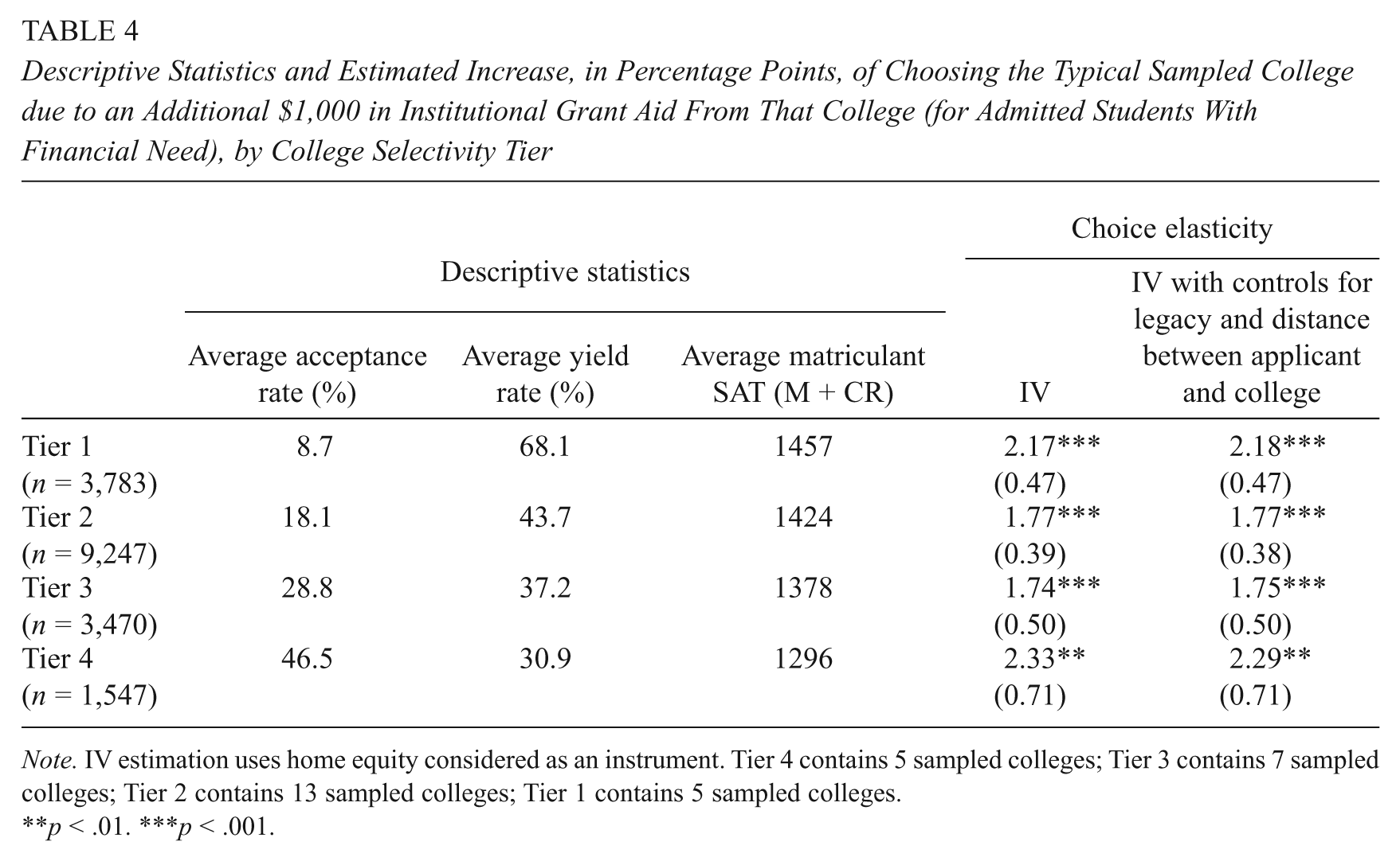
Creating four instruments (EST_HOMEE QUITY *TIER1, EST_HOMEEQUITY*TIER2, etc.) for four endogenous variables (INSTGRANT*TIER1, INSTGRANT*TIER2, etc.), I adopt an IV estimation strategy similar to that presented in Equations 3 through 9 to obtain unbiased estimates of choice elasticity in each of the four selectivity tiers. In Table 4, I show the average acceptance rates (Column 1), average yield rates (Column 2), and the average SAT composite scores (Column 3) in each of the four selectivity tiers, as well as the accompanying choice elasticity estimates. Choice elasticity estimates are fairly stable across the four selectivity tiers, ranging from 1.75 in Tier 3 to 2.29 in Tier 4. Through a post hoc generalized linear hypothesis test, I cannot reject the hypothesis that these four choice elasticity estimates differ from the overall sample choice elasticity estimate of 1.66 (F = 1.51, p = .20). This provides compelling evidence that EST_HOMEEQUITY is a robust instrument for institutional grant aid across the entire sample, when controlling for the fixed effects of colleges and students, in addition to LEGACY and GEODIST. Moreover, these findings are consistent with the hypothesis that choice elasticity is unrelated to college selectivity, suggesting that this article’s findings may be generalizable to a much broader set of colleges than those included in my sample.

Table 4

Descriptive Statistics and Estimated Increase, in Percentage Points, of Choosing the Typical Sampled College due to an Additional $1,000 in Institutional Grant Aid From That College (for Admitted Students With Financial Need), by College Selectivity Tier

	Descriptive statistics			Choice elasticity
	Average acceptance rate (%)	Average yield rate (%)	Average matriculant SAT (M + CR)	IV	IV with controls for legacy and distance between applicant and college
Tier 1	8.7	68.1	1457	2.17***	2.18***
(n = 3,783)				(0.47)	(0.47)
Tier 2	18.1	43.7	1424	1.77***	1.77***
(n = 9,247)				(0.39)	(0.38)
Tier 3	28.8	37.2	1378	1.74***	1.75***
(n = 3,470)				(0.50)	(0.50)
Tier 4	46.5	30.9	1296	2.33**	2.29**
(n = 1,547)				(0.71)	(0.71)

Note. IV estimation uses home equity considered as an instrument. Tier 4 contains 5 sampled colleges; Tier 3 contains 7 sampled colleges; Tier 2 contains 13 sampled colleges; Tier 1 contains 5 sampled colleges.

p < .01. ***p < .001.

Footnotes

Acknowledgements

The author gratefully acknowledges the feedback regarding this project from Ann Birk, Dominic Brewer, Kristine Dillon, Bridget Terry Long, Steve Minicucci, and John Willett, as well as three anonymous reviewers. The author takes full responsibility for any errors in this article. Statements in this article do not necessarily reflect the position of the College Board.

Notes

Author

MICHAEL HURWITZ is an associate research scientist at the College Board’s Advocacy & Policy Center. His research focuses on higher education access. He can be reached at 1233 20th St., NW, Suite 600 Washington, DC 20036-2375 or mhurwitz@collegeboard.org.

References

Aitken

N. D.

(1982). College student performance, satisfaction and retention: Specification and estimation of a structural model. The Journal of Higher Education, 53(1), 32–50.

Allison

(2005). Fixed effects regression methods for longitudinal data using SAS®. Cary, NC: SAS Institute Inc.

Angrist

J. D.

Pischke

J. S.

(2009). Mostly harmless econometrics: An empiricist’s companion. Princeton, NJ: Princeton University Press.

Avery

Glickman

Hoxby

C. M.

Metrick

(2005). A revealed preference ranking of U.S. colleges and universities (NBER Working Paper 10803). Retrieved from http://www.nber.org/papers/w10803.pdf

Avery

Hoxby

C. M.

(2003). Do and should financial aid packages affect students’ college choices? (NBER Working Paper 9482). Retrieved from http://www.nber.org/papers/w9482.pdf

Baum

Payea

(2011). Trends in student aid 2011. New York, NY: The College Board Advocacy & Policy Center.

Betts

J. R.

Fairlie

R. W.

(2001). Explaining ethnic, racial, and immigrant differences in private school attendance. Journal of Urban Economics, 50(1), 26–51.

Bound

Hershbein

Long

B. T.

(2009). Playing the admissions game: Student reactions to increasing college competition. Journal of Economic Perspectives, 23(4), 119–146.

Brint

(2010, January 10). Amid recession, some college admissions policies look at students’ wealth. The Washington Post. Retrieved from http://www.washingtonpost.com/wp-dyn/content/article/2010/01/08/AR2010010803584.html

10.

College Board. (2007). Meeting college costs, 2008 edition. New York, NY: Author.

11.

Dale

S. B.

Krueger

A. B.

(2002). Estimating the payoff to attending a more selective college: An application of selection on observables and unobservables. The Quarterly Journal of Economics, 117(4), 1491–1527.

12.

DeNavas-Walt

Proctor

B. D.

Smith

J. C.

(2010). U.S. Census Bureau, current population reports, P60-238, income, poverty, and health insurance coverage in the United States: 2009. Washington, DC: U.S. Government Printing Office.

13.

Dynarski

S. M.

(2000). Hope for whom? Financial aid for the middle class and its impact on college attendance. National Tax Journal, 53(3), 629–661.

14.

Dynarski

S. M.

(2003). Does aid matter? Measuring the effect of student aid on college attendance and completion. The American Economic Review, 93(1), 279–288.

15.

Ehrenberg

R. G.

(2000). Tuition rising: Why college costs so much. Cambridge, MA: Harvard University Press.

16.

Eide

Brewer

D. J.

Ehrenberg

R. G.

(1998). Does it pay to attend an elite private college? Evidence on the effects of undergraduate college quality on graduate school attendance. Economics of Education Review, 17(4), 371–376.

17.

Entwisle

D. R.

Astone

N. M.

(1994). Some practical guidelines for measuring youth’s race/ethnicity and socioeconomic status. Child Development, 65(6), 1521–1540.

18.

Fitzsimmons

W. R.

McGrath

M. E.

Donahue

S. C.

(2009). Harvard College Office of Admissions and financial aid 2009 newsletter. Retrieved from http://admissions.college.harvard.edu/counselors/gc_newsletter_fall2009.pdf

19.

Geyer

C. J.

Thompson

E. A.

(1992). Constrained Monte Carlo maximum likelihood for dependent data. Journal of the Royal Statistical Society. Series B (Methodological), 54(3), 657–699.

20.

Griffith

A. L.

Rothstein

D. S.

(2009). Can’t get there from here: The decision to apply to a selective college. Economics of Education Review, 28(5), 620–628.

21.

Hill

C. B.

Winston

G. C.

(2010). Low-income students and highly selective private colleges: Geography, searching, and recruiting. Economics of Education Review, 29, 495–503.

22.

Horrace

W. C.

Oaxaca

R. L.

(2006). Results on the bias and inconsistency of ordinary least squares for the linear probability model. Economics Letters, 90(3), 321–327.

23.

Hoxby

C. M.

(2009). The changing selectivity of American colleges. Journal of Economic Perspectives, 23(4), 95–118.

24.

Hoxby

C. M.

Long

(1999). Explaining rising income and wage inequality among the college educated (NBER Working Paper 6873). Retrieved from http://www.nber.org/papers/w6873.pdf

25.

Hurwitz

(2011). The impact of legacy status on undergraduate admissions at elite colleges and universities. Economics of Education Review, 30(3), 480–492.

26.

Ishida

Spilerman

(1997). Educational credentials and promotion chances in Japanese and American organizations. American Sociological Review, 62(6), 866–882.

27.

Kelley

(2010, December 9). Cornell to match financial aid offers of peer universities. Cornell University Chronicle Online. Retrieved from http://www.news.cornell.edu/stories/Dec10/AidMatch.html

28.

Kim

(2010). Early decision and financial aid competition among need-blind colleges and universities. Journal of Public Economics, 94(5-6), 410–420.

29.

Lentz

B. F.

Laband

D. N.

(1989). Why so many children of doctors become doctors: Nepotism vs. human capital transfers. The Journal of Human Resources, 24(3), 396–413.

30.

Lewin

(2010, December 17). Unease grows about future of financing for Pell grants. The New York Times. Retrieved from http://www.nytimes.com/2010/12/18/education/18pell.html

31.

Linsenmeier

D. M.

Rosen

H. S.

Rouse

C. E.

(2006). Financial aid packages and college enrollment decisions: An econometric case study. Review of Economics and Statistics, 88(1), 126–145.

32.

Long

B. T.

(2004). How have college decisions changed over time? An application of the conditional logistic choice model. Journal of Econometrics, 121(1-2), 271–296.

33.

Manski

Wise

(1983). College choice in America. Cambridge, MA: Harvard University Press.

34.

McDonough

P. M.

(1997). Choosing colleges: How social class and schools structure opportunity. Albany, NY: State University of New York Press.

35.

Monks

(2009). The impact of merit-based financial aid on college enrollment: A field experiment. Economics of Education Review, 28(1), 99–106.

36.

Murnane

R. J.

Willett

J. B.

(2011). Method matters: Improving causal inference in educational and social science research. Oxford, UK: Oxford University Press.

37.

Nurnberg

Schapiro

Zimmerman

(2010). Students choosing colleges: Understanding the matriculation decision at a highly selective private institution? (NBER Working Paper 15772). Retrieved from http://www.nber.org/papers/w15772.pdf

38.

Okun

M. A.

Levy

Karoly

Ruehlman

(2009). Dispositional happiness and college student GPA: Unpacking a null relation. Journal of Research in Personality, 43(4), 711–715.

39.

Perna

L. W.

(2006). Studying college access and choice: A proposed conceptual model. Higher Education: Handbook of Theory and Research, 21, 99–157.

40.

Rimer

Finder

(2007, December 11). Harvard to aid students high in middle class. The New York Times. Retrieved from http://www.nytimes.com/2007/12/11/education/11harvard.html?pagewanted=print

41.

Roberts

(2011, September 15). UC officials take pay raises; warn of doubling tuition. NBC Bay Area News. Retrieved from http://www.nbcbayarea.com/news/local/UC-Officials-Take-Pay-Raises-While-Warning-of-Doubling-Tuition–129901743.html

42.

Roman

(2008, January 15). Yale overhauls financial aid; Reform targets middle class. Yale Daily News. Retrieved from http://www.yaledailynews.com/news/2008/jan/15/yale-overhauls-financial-aid-reform-targets/

43.

Sacerdote

(2001). Peer effects with random assignment: Results for Dartmouth roommates. The Quarterly Journal of Economics, 116(2), 681–704.

44.

Tedeschi

(2009, April 3). College tuition not on the house. The New York Times. Retrieved from http://www.nytimes.com/2009/04/05/realestate/05mort.html

45.

U.S. News and World Report Best Colleges 2010. (2009).

46.

U.S. News and World Report Best Colleges 2011. (2010).

47.

van der Klaauw

(2002). Estimating the effect of financial aid offers on college enrollment: A regression-discontinuity approach. International Economic Review, 43(4), 1249–1287.

48.

Winston

G. G.

(1999). Subsidies, hierarchy and peers: The awkward economics of higher education. Journal of Economic Perspectives, 13(1), 13–36.

49.

Wong

G. W.

(2005, December 12). Early decision action plan: Your child has been accepted to the college of their dreams—but are you sure you can afford it? CNNMoney.com . Retrieved http://money.cnn.com/2005/12/09/pf/college/early_decision/index.htm

50.

Zimmerman

(2003). Peer effects in academic outcomes: Evidence from a natural experiment. Review of Economics and Statistics, 85(1), 9–23.